TECHNICAL UNIVERSITY OF CLUJ-NAPOCA
ACTA TECHNICA NAPOCENSIS
Series: Applied Mathematics, Mechanics, and Engineering Vol. 61, Issue IV, November, 2018
THE DYNAMIC STUDY OF AN ASSEMBLY CAM
─
SPRING
Iuliu NEGREAN, Adina CRIŞAN
Abstract: The purpose of the present paper consists in highlighting of the higher order accelerations that occur in
the oscillatory motion of a spring as well as in the rotational motion of a cam, both of them part of a cam and follower mechanism. The cam is acted by means of an electrical engine, the rotational motion of the cam being the source of the oscillatory motion performed by the spring. Because the higher order accelerations are characteristic to sudden motions, this paper will demonstrate that the perturbing force applied to the spring as well as the torque are both characterized by a variation law with respect time. The study conducted on the accelerations of higher order will be accomplished by the instrumentality of polynomial interpolation functions of higher order. The results will have at basis, in the future papers, measurements performed on the spring and cam which consists in determining the linear velocity of the spring and of the linear velocity of a point from the circular cam ring periphery respectively.
Key words: mechanics, kinematics, cam and spring, advanced notions, dynamics equations.
1. INTRODUCTION
The cam – follower system represents an extremely versatile machine element which allows for almost any specified motion to be performed. This type of mechanism can be used in a wide variety of industrial applications, especially the one which require a higher level of accuracy and repeatability or when is a need for operating at high speeds.
The simple motions, such as rotation or translation, can be transformed into any other type of motions by using cam mechanisms, these providing the simplest and most compact way to transform motions. The mechanism usually consists of two moving elements, the cam and a follower, mounted on a fixed frame.
A cam and follower mechanism is a profiled shape, mounted on a shaft that imparts a predetermined motion to another element called the follower (Fig.1). Cams are converting the rotation motion into linear motion. So, when the cam performs a rotation motion, the follower rises and falls in a process known as reciprocating motion, but in the same time it maintains contact with the cam through the force of gravity or by means of a spring. The stroke is the total range of movement produced by the cam. The movement of the follower is restricted to a predetermined
pattern by means of a slideway, the range of motion depending on the distance measured from the shaft, which is supporting the cam, to the upper and lower points of the rotation circle.
Fig. 1 The cam and follower system The cams are usually designed in different individual shapes in order to generate specific types of motion. There is a large variety of cams in what concerns the shapes and sizes, but the most common used in practice are the circular cams with an off-center hole, pear shaped and snail shaped cams. When the cams rotate, the followers carry out a reciprocate motion according to the profile of the cam. For example, in case of the cams characterized by a circular shape, sometimes referred to as eccentric cams, the movement will be characterized by a smooth rise and fall, with no pause, motion also known as harmonic motion.
R e
C
R l−
L 0
O A0′ x0
0 y
2. THE KINEMATIC STUDY
The mechanism consisting of a cam and a follower is usually defined by one degree of freedom which can be represented by the rotation angle ϕ of the cam or by the linear displacement of the follower, x.
Fig. 2 The geometry of cam and follower The motion of a point on the periphery on the cam circle can be described using the polynomial interpolation functions.
According to the research of the main author, example [12] – [15], polynomial interpolation functions can be expressed in a general form as:
( )
( )
( ) (
(
)
)
( )(
)
(
)
( )
(
)
τ ττ
τ τ δ τ
+ −
−
+ −
−
=
⎧ − ⎫
= − ⋅ ⋅ +
⎪ ⎪
⋅ +
⎪ ⎪
⎨ − ⎬
⎪+ ⋅ + ⋅ ⋅ ⎪
⎪ ⋅ + − ⎪
⎩
∑
⎭!
! !
p 1
m p m
p i
ji ji 1
i
p 1 m p p k i 1
ji p jik
k 1 i
q 1 q
t p 1
q a
t p 1 p k
(1)
In the expression presented above, m represents the deriving order of the polynomial function (
≥ , = , , , ,K
m 2 m 2 3 4 5 ), p = 0 → m ,
= →
j 1 n are the degrees of freedom of the analyzed mechanical system. In the same equation, δp represents the space travelled during
i
t period of time, being defined by the following identity: δp =
{
(
0 p 0 1 p 1, =) (
; ; ≥)
}
.If in case of the real interpolation function, δp represents the space travelled during time interval
i
t , for the normalized function, it travels a space of unity length in a given time interval. Also,
= →
i 1 s defines the intervals of motion trajectories, τ is the actual time variable
τ τ∈[ i 1− τi], and ti = −τ τi i 1− is the actual time corresponding to each trajectory interval ( )i . For every trajectory interval
(
i 1= →s)
,(
m 1+)
represents the number of unknowns, defined as:⎧⎨
( )
= → ⎛⎜( )− ⎞⎟ = → ⎫⎬⎝ ⎠
⎩ ; ⎭
m
jik ji 1
a for k 1 m q for i 2 s ; (2)
where
( )
ajik are the integration constants, as well( )
−
⎛ ⎞ ⎜ ⎟ ⎝ ⎠
m ji 1
q the generalized accelerations of
( )
m order. To determine the unknowns defined by the expression (2), is required to apply geometrical and kinematical constraints [11], [15] – [18]:( )
( )( )
( )( )
( )
( )
( )
( )
( )
( )
m p m
0 j0 s js js
2 ji
m p m p ji ji 1 i
i
q p 0 m q q
q generalized accelerations
q q p 0 m
continuity conditions all conditions are applied to each
where i 1 s 1
τ τ
τ τ
τ
τ
−
− −
+ −
+
⎧ ⇒ = → ⇒⎧⎪ ⎫⎪
⎪ ⎨ ⎬
⎪ ⎪
⎩ ⎭
⎪
⎪ ⎧ ⎫
⎪ ⎪ − ⎪
⎪ ⎪ ⎪
⎧ ⎫
⎨ ⎪⎪ ⎪⎪
⎪ = = → ⎪
⎪ ⇒⎨⎨ ⎬⎬
⎪ ⎪⎪ ⎪⎪
⎩ ⎭
⎪ ⎪ ⎪
⎪ ⎪
= → −
⎪ ⎪
⎩ ⎭
⎩
, ; ,
,
⎫ ⎪ ⎪ ⎪ ⎪ ⎪ ⎬ ⎪ ⎪ ⎪
⎪ ⎪
⎪ ⎪⎭
(3)
The continuity conditions from (3) are applied to each
( )
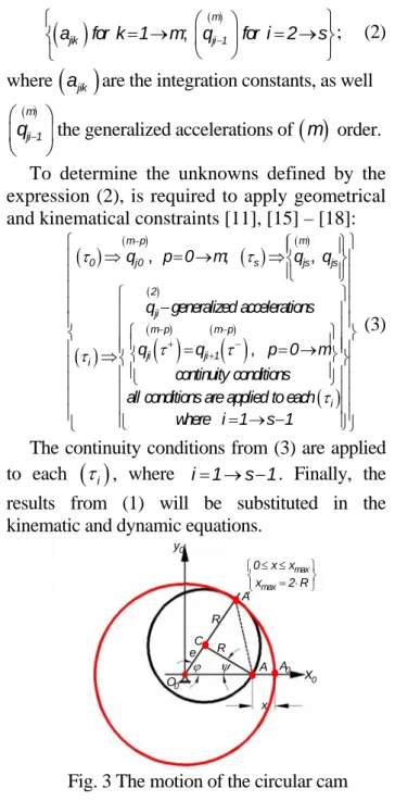
τi , where i 1= → −s 1. Finally, the results from (1) will be substituted in the kinematic and dynamic equations.Fig. 3 The motion of the circular cam When the polynomial interpolation functions of third order are used, is achieved continuity in position and velocity, but accelerations are presenting in some cases discontinuity intervals, which require the use of higher order polynomials. There can be defined different types of trajectories that can be described by the cam – follower mechanism in the configuration space depending on the constraints that are imposed by the work process. According to [12], [13] the kinematical constraints that are applied in case of polynomial functions of fifth order, for the follower are:
( )
0 0 j0 0 j00 j0 0 j0
h x v x
a x a x
τ
⇒⎨⎧⎪ = = ⎫⎪⎬= =
⎪ ⎪
⎩ ⎭
& && && &&&&
; ;
; ; (4)
0
x
ψ A
e R
0
y
R C
x
0
A
0
O
max max
0 x x
x 2 R
≤ ≤
⎧ ⎫
⎨ = ⋅ ⎬
⎩ ⎭
ϕ
A′
( )k
e
C
max
x
R L
0
A
(R l+ )
0
O A0′ x0
0
( )
τn ⇒{
hn=xjn; a&& &&&&n = xjn}
; (5)( )
( )
( ) ( )
( )
( )
( )
i ji
i i i 1 i i 1
i i 1
a x i 1 n 1
h t h t v t v t
a t a t
τ + − + −
+ + + − + = = → − ⎧ ⎪ ⇒⎨ = = ⎪ = ⎩ && & & ;
; ; (6)
The time functions for generalized variables of fifth order are defined with the expressions:
( )
(
i)
( )
(
i 1)
( )
ji ji i 1 ji i
i i
x x x
t t
τ τ τ τ
τ τ − τ
−
− −
= ⋅ + ⋅
&&&& &&&& &&&& ; (7) (8)
( )
(
i)
2(
i 1)
2ji ji 1 ji ji1
i i
x x x a
2 t 2 t
τ τ τ τ
τ −
−
− −
= − ⋅ + ⋅ +
⋅ ⋅
&&& &&&& &&&& ;(9)
( ) (
)
(
)
3 i
ji ji 1
i 3 i 1
ji ji1 ji 2 i
x x
6 t
x a a
6 t τ τ τ τ τ τ − − ⎧ − ⎫ = ⋅ + ⎪ ⎪ ⎪ ⋅ ⎪ ⎨ − ⎬ ⎪+ ⋅ + ⋅ + ⎪ ⎪ ⋅ ⎪ ⎩ ⎭ && &&&& &&&&
; (10)
( )
(
)
(
)
4 i
ji ji 1
i
4 2
i 1
ji ji1 ji2 ji3 i
x x
24 t
x a a a
24 t 2
τ τ τ
τ τ τ τ
− − ⎧ − ⎫ = − ⋅ + ⎪ ⎪ ⎪ ⋅ ⎪ ⎨ ⎬ − ⎪+ ⋅ + ⋅ + ⋅ + ⎪ ⎪ ⋅ ⎪ ⎩ ⎭ & &&&& &&&& ; (11)
( ) (
)
(
)
5 ijik ji 1k
i 5 3 i 1 jik jik1 i 2
jik 2 jik 3 jik 4
q x
120 t
x a
120 t 6
a a a
2
τ τ τ
τ τ τ
τ τ − − ⎧ − ⎫ = ⋅ + ⎪ ⎪ ⋅ ⎪ ⎪ ⎪ − ⎪ ⎨+ ⋅ + ⋅ +⎬ ⎪ ⋅ ⎪ ⎪ ⎪ + ⋅ + ⋅ + ⎪ ⎪ ⎩ ⎭ &&&&
&&&& ; (12)
The kinematical constraints which are applied for the circular cam, for i 1= →n, are:
( )
( ) ( ) ( )
4 1 1
i i 1
i 4 i 1 4 i
i i
t t
τ τ τ τ
ϕ τ ϕ − ϕ
−
⎧ = − ⋅ + − ⋅ ⎫
⎨ ⎬
⎩ ⎭; (13)
( ) ( )
(
)
( )(
)
( ) 1 2 3 1 ii 4 i 1
i 2 1 i 1 i i 4 i 2 t a 2 t τ τ
ϕ τ ϕ
τ τ ϕ
− − ⎧ − ⎫ = − ⋅ + ⎪ ⎪ ⋅ ⎪ ⎪ ⎨ ⎬ − ⎪ + ⋅ + ⎪ ⎪ ⋅ ⎪ ⎩ ⎭
; (14)
( ) ( )
(
)
( )(
)
( ) 1 2 3 2 1 ii 4 i 1
i
3 1
i 1
i i i
4 i 6 t a a 6 t τ τ
ϕ τ ϕ
τ τ ϕ τ − − ⎧ − ⎫ = ⋅ + ⎪ ⎪ ⋅ ⎪ ⎪ ⎨ ⎬ − ⎪+ ⋅ + ⋅ + ⎪ ⎪ ⋅ ⎪ ⎩ ⎭
; (15)
( ) ( )
(
)
( )(
)
( ) 1 2 3 4 41 1 1
i i 1
i 4 i 1 4 i
i i
i 2
i i
24 t 24 t
a
a a
2
τ τ τ τ
ϕ τ ϕ ϕ
τ τ − − ⎧ − − ⎫ ⎪ = − ⋅ + ⋅ +⎪ ⎪ ⋅ ⋅ ⎪ ⎨ ⎬ ⎪ ⎪ + ⋅ + ⋅ + ⎪ ⎪ ⎩ ⎭
; (16)
( )
(
)
( )(
)
( )1 2
3 4
5 1 5 1
i i 1
i 4 i 1 4 i
i i
i 3 i 2
i i
120 t 120 t
a a
a a
6 2
τ τ τ τ
ϕ τ ϕ ϕ
τ τ τ
− − ⎧ − − ⎫ ⎪ = ⋅ + ⋅ +⎪ ⎪ ⋅ ⋅ ⎪ ⎨ ⎬ ⎪ ⎪ + ⋅ + ⋅ + ⋅ + ⎪ ⎪ ⎩ ⎭
; (17)
(
t1)
( )
( ) ( )
0(
0)
0 1
1 0 1
; ;
:
;
ϕ τ ϕ τ
τ τ
ϕ τ ϕ τ τ
⎧ ⎫ ⎪ ⎪ ⎯⎯→ ⎨ ⎬ − ⎪ ⎪ ⎩ ⎭ &
& ; (18)
(
t2)
( )
( )
1( )
( )
11 2
2 2
; ;
:
;
ϕ τ ϕ τ
τ τ
ϕ τ ϕ τ
⎧ ⎫ ⎪ ⎪ ⎯⎯→ ⎨ ⎬ ⎪ ⎪ ⎩ ⎭ &
& ; (19)
(
)
( ) ( )
( ) ( )
i i 1 i 1
t
i 1 i
i i
; ;
:
;
ϕ τ ϕ τ
τ τ
ϕ τ ϕ τ
− − − ⎧ ⎫ ⎪ ⎪ ⎯⎯→ ⎨ ⎬ ⎪ ⎪ ⎩ ⎭ &
& ; (20)
(
)
( ) ( )
( ) ( )
n n 1 n 1
t
n 1 n
n n
; ;
:
;
ϕ τ ϕ τ
τ τ
ϕ τ ϕ τ
− − − ⎧ ⎫ ⎪ ⎪ ⎯⎯→ ⎨ ⎬ ⎪ ⎪ ⎩ ⎭ &
& ; (21)
In the following are established the kinematical expressions between the linear displacement
( )
x τ of the spring and the rotation angle ϕ τ( ) which characterizes the rotation motion of the cam. According to Fig.1-3, are determined the trigonometric functions for ψ τ( ) an angle whose value is dependent of the rotation angle ϕ τ( ):
s
[
( )]
e s[
( )]
R
ψ τ = ⋅ ϕ τ ; (22)
( )
[
]
1 2 2 2[
( )]
c R e s
R
ψ τ = ± ⋅ − ⋅ ϕ τ ; (23)
Also is determined the dependence between the angle ϕ τ( )and linear displacementx( )τ such as:
( ) ( ) ( )
R e x+ − τ = ⋅e cϕ τ + ⋅R cψ τ ; (24)
Expression (23) is substituted in (24), resulting:
( )
[ ]
( ) 2 2 2[
( )]
R e x+ − τ = ⋅e cϕ τ + R − ⋅e s ϕ τ ; (25)
( )
(
R e x τ)
e cϕ τ[ ]
( ) 2 R2 e s2 2[
ϕ τ( )]
⎡ + − − ⋅ ⎤ = − ⋅
⎣ ⎦ ; (26)
( )
( )2 2 ( ( ))
[ ]
( ) 2R e x+ − τ + − ⋅ ⋅ + −e 2 e R e xτ ⋅cϕ τ =R ; (27) from where the value of angle ϕ τ( ) is determined:
( )
[
]
((
)(
( ))
( ))
( )[
]
( )(
( ))
( )( ) 2 2 2 2 2x 2 e R e x
c
2e R e x
x 2 e R e x
s 1
4e R e x
τ ϕ τ τ τ ϕ τ τ ⎧ + ⋅ + ⋅ − = ⎪ ⋅ + − ⎪ ⎨ ⎡ ⎤ ⎪ = −⎣ + ⋅ + ⋅ − ⎦ ⎪ ⋅ + − ⎩ (28)
( ) Atan2 s
{
[
( )]
; c[
( )]
}
f x[
( )]
ϕ τ = ϕ τ ϕ τ = τ (29) According to expressions previously presented, it results that assembly cam – spring is defined by an independent parameter: ϕ τ( ) or x( )τ3. THE DYNAMICS OF THE EQUIPMENT
The main purpose of the present paper is to establish the time variation law for the perturbing force that generates the motion of a cam and follower mechanism. The system which is going to be analyzed consists of a rotating cam and a translating roller type follower (Fig.1, Fig. 2).
The cam profile is represented by a circle of radiusR. The rotation center of the cam is situated eccentric from the geometrical center, at distancee. The cam produces a smooth motion also known as harmonic motion (Fig. 3).
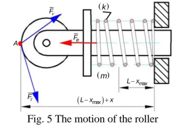
Fig. 4 The distribution of forces for the cam The follower consists of a spring characterized by the elastic constant k and undistorted length L. The assembly is situated in the vertical plane z 0= , the cam being attached on a shaft and acted by means of an electrical engine. A follower with a small roller attached, pushes against the cam (Fig. 4).
Fig. 5 The motion of the roller
As the shaft rotates, the roller follows the cam profile causing the follower to rise or to fall. The rotation motion of the cam will generate a perturbing force in the theoretical contact point
which will impose an oscillatory motion to the spring, around x0 axis (see Fig. 4).
The fundamental theorems that characterize the motion of the equipment are represented by the theorem of motion of the center in case of the spring and the theorem of angular momentum for the circular cam. These theorems are known, in accordance with scientific literature, [8], [10]. The main objective of this section consists in presenting some reformulations of the theorems, applied for a rigid body involved in general motion, in this case the circular cam (see Fig.3). According to [10], [12], the theorem of the motion of the mass center, applied for the component of the system engaged in a oscillatory motion, in this case the spring, can be written as:
( ) ( ) ( ) ( )
r C r C r C
M a⋅ τ =M v⋅& τ =M r⋅&& τ =R τ ; (30) where Mr represents the mass of the spring,
C C C
a = =v& &&r the acceleration which characterizes
the motion of the spring’s mass center and finally, R is the resultant vector of active forces applied on the elastic spring.
The next component of the analyzed system is represented by the source of motion, which is, in this case the circular cam. According to Fig. 3 this component (the cam) is engaged motion by an electrical engine, performing a rotation motion around a fixed axis which passes through a point
0
O positioned eccentrically from the geometrical center of the cam and denoted with C.
The motion of the cam is studied by considering the general form of angular momentum theorem, in case of a rigid body which is performing a general motion:
( ) ( ) ( ) ( ) [ ]( ) [ ] ( ) ( ) ( )( ) [ ]( ) [ ] ( ) ( )
C C C S S
0 S 0 T
S S
C C S
0 T S
S S
K r M a I I
r M a R I R
t R I R
τ ε τ ω τ ω τ
τ τ ε τ
ω τ τ τ ω τ
∗ ∗
∗
∗
⎧ = × ⋅ + ⋅ + × ⋅ =⎫
⎪ ⎪
⎪ ⎪
⎨ = × ⋅ + ⋅ ⋅ ⋅ + ⎬
⎪ ⎪
+ × ⋅ ⋅ ⋅
⎪ ⎪
⎩ ⎭
&
(31)
( ) ( ) ( ) ( ) ( ) ( )
S S C
I∗ τ ε τ⋅ +ω τ ×I∗ τ ω τ⋅ =M τ
. (32) The expression (32) represents the theorem of angular momentum with respect to mass center. where, MC is the resultant moment of the active forces relative to the mass center of the cam,
[ ]( )
0
S R t is the resultant rotation matrix between the mobile system attached to cam and the fixed
Fν
Fτ
A
(L x− max)+x
max
L x−
e
F
( )m
( )k
0
x
M g⋅ ψ A
A′
Fν
e R 0
y
R
Fτ
m
M C
x
0
A
ϕ
0
O
max max
0 x x
x 2 R
≤ ≤
⎧ ⎫
⎨ = ⋅ ⎬
system, and finally, I tS∗( )represents the inertial tensor, axial–centrifugal, relative to mass center. If applied in case of the circular cam, which means by applying the constraints specific to the rotation around a fixed axis, expression (32) is:
( ) ( )
Z Z z
K& τ =M I= ⋅ϕ τ&& ; (33) where ϕ&& is the angular acceleration of the cam and Iz is expressed with the following formula:
c 2 2
z M R c
I M R
2
⋅
= + ⋅ ; (34) In the expression (34), Iz is the axial moment of inertia of the cam with respect to the rotation axis, Mcam is mass of the cam and R its radius. As mentioned before, the mechanical system consisting of a cam and a follower is characterized by a single degree of freedom which can be the either the angle of rotation ϕ or the linear displacement x, which are unknown. The motion laws for the two components of the analyzed system (cam and follower) are determined by solving the differential equations:
( ) ( ) ( )
r p
M x⋅&&τ = ⋅k x τ −F τ ; (35)
where Fp( )τ = ⋅Fν ⎣⎡c
[
ψ τ( )]
+ ⋅μ ψ τs[
( )]
⎤⎦; (36) In expression (36), Fp( )τ is the perturbing force and is characterized by a time variation law, Fν represents the normal downforce at the contact surface between the circular cam and spring andμ is the sliding friction coefficient between the contour of the cylindrical cam and the roller situated at the extremity of the follower.
The expression (35) represents the differential equation of motion that characterizes the movement of the follower (spring). By experimental measurements, the linear acceleration of the follower x&& can be determined by using the polynomial interpolation functions which leads to the defining of the time variation law characteristic to the perturbing force.
The polynomial interpolation functions for the rotation angle ϕ along with their higher order time derivatives are determined for the circular cam as well. Also, the differential equation of motion for the circular cam is written as follows:
( )
(
)
(
[ ]
( )[
( )]
)
( )
[
]
( ) ( )cam m z
F R e x s c
M g c M I
ν τ ψ τ μ ψ τ
ϕ τ τ ϕ τ
⎧ ⋅ + − − ⋅ −⎫
⎪ ⎪
⎨ ⎬
⎪ − ⋅ ⋅ + = ⋅ ⎪
⎩ && ⎭
(37)
In the equation presented above, e represents the eccentricity, Mm the driving moment, x is the displacement of the contact point between the cam and follower and ψ is an angle which according to Fig. 3 is dependent on the rotation angle ϕ.
The equation (37) is further used to determine the time variation law for the driving moment Mm( )τ which imparts rotation motion to the circular cam and withal the oscillatory motion to the arc as well.
4. CONCLUSIONS
By means of the researches of the author, in the first two sections of this paper formulations concerning the classical theorems from dynamics were presented, with application for a system consisting of a circular cam and a follower. So, the theorem of the mass center, and theorem of the angular momentum, were defined in the explicit form and applied for the cam and follower mechanical system.
The purpose of the present paper consists in highlighting of the higher order accelerations that occur in the oscillatory motion of a spring as well as in the rotational motion of a cam, both of them part of a cam and follower mechanism. The cam is acted by means of an electrical engine, the rotational motion of the cam being the source of the oscillatory motion performed by the spring. Because the higher order accelerations are characteristic to sudden motions, this paper will demonstrate that the perturbing force applied to the spring as well as the torque are both characterized by a variation law with respect to time. The study conducted on the accelerations of higher order will be accomplished by the instrumentality of polynomial interpolation functions of higher order. The results were based on the measurements performed on the spring and cam which consists in determining the linear velocity of the spring and the linear velocity of a point from the circular contour of the physical cam.
5. REFERENCES
[1] R.P. Paul and H. Zhong, 1984, Robot Motion
Second International Symposium on Robotics Research, Kyoto, Japan, August. [2]R.E. Parkin, 1991, Applied Robotic Analysis,
Prentice Hall, Englewood Cliffs, NJ.
[3]L.Sciavicco and B. Siciliano, 2008, Robotics:
Modeling, Planning, and Control, McGraw-Hill, New York.
[4]Negrean I., Vușcan I., Haiduc N., Robotics.
Kinematic and Dynamic Modeling, Editura Didacticăși Pedagogică, R.A. București, 1998
[5]J.J. Craig, 2005, Introduction to Robotics:
Mechanics and Control, 3rd edition, Pearson Prentice Hall, Upper Saddle River, NJ.
[6]Appell, P., Sur une forme générale des
equations de la dynamique, Paris, 1899. [7]Negrean, I., Negrean, D. C., The Acceleration
Energy to Robot Dynamics, International Conference on Automation, Quality and Testing, Robotics, AQTR 2002, May 23-25, Cluj-Napoca, Tome II, pp. 59-64
[8]Negrean I., Mecanică avansată în Robotică, ISBN 978-973-662-420-9, UT Press, Cluj-Napoca, 2008.
[9]Negrean, I., Energies of Acceleration in
Advanced Robotics Dynamics, Applied Mechanics and Materials, ISSN: 1662-7482, vol 762, pp 67-73 Submitted: 2014-08-05 ©(2015)TransTech Publications Switzerland [10]Negrean I., New Formulations on
Acceleration Energy in Analytical Dynamics,
Applied Mechanics and Materials, vol. 823 pp 43-48 © (2016) TransTech Publications Switzerland Revised: 2015-09,
[11]Negrean I., New Formulations on Motion
Equations in Analytical Dynamics, Applied Mechanics and Materials, vol. 823 (2016), pp 49-54 © (2016) TransTech Publications. [12]Negrean I., Advanced Notions in Analytical
Dynamics of Systems, Acta Technica Napocensis, Series: Applied Mathematics, Mechanics and Engineering, Vol. 60, Issue IV, November. 2017, pg. 491-502.
[13]Negrean I., Advanced Equations in Analytical
Dynamics of Systems, Acta Technica Napocensis, Series: Applied Mathematics, Mechanics and Engineering, Vol. 60, Issue IV, November 2017, pg. 503-514.
[14]Negrean I., New Approaches on Notions
from Advanced Mechanics, Acta Technica Napocensis, Series: Applied Mathematics, Mechanics and Engineering, Vol. 61, Issue II, June 2018, pg. 149-158.
[15]Negrean I., Generalized Forces in
Analytical Dynamic of Systems, Acta Technica Napocensis, Series: Applied Mathematics, Mechanics and Engineering, Vol. 61, Issue II, June 2018, pg. 357-368. [16]Fu K., Gonzales R., Lee C., Control,
Sensing, Vision and Intelligence, McGraw-Hill Book Co., International Edition, 1987
Studiul dinamic al unui ansamblu camă – resort
Rezumat: Scopul principal al prezentei lucrări îl reprezintă evidențierea accelerațiilor de ordin superior in
mișcarea oscilatorie a unui resort elastic, respectiv în mișcarea de rotație a unei came circulare, ambele fiind componente ale unui sistem de tip camă – palpator, în care cama circulară reprezintă sursa generatoare a mișcării oscilatorii a resortului. Prin aplicarea accelerațiilor de ordin superior ce corespund mișcărilor rapide, în cadrul acestei lucrări se va arata ca forța perturbatoare aplicată resortului elastic, precum și momentul motor sunt caracterizate print-o lege de variație în raport cu timpul, a cărei determinare este unul dintre obiectivele lucrării de față. Studiul accelerațiilor de ordin superior se va realiza prin aplicarea funcțiilor polinomiale de interpolare de ordin superior. Rezultatele obținute vor avea la bază, în lucrări viitoare, măsurători experimentale asupra accelerației liniare a resortului, respectiv a vitezei liniare ce caracterizează mișcarea unui punct situat pe periferia camei circulare.
Iuliu NEGREAN Professor Ph.D., Member of the Academy of Technical Sciences of Romania, Director of Department of Mechanical Systems Engineering, Technical University of Cluj-Napoca, [email protected], http://users.utcluj.ro/~inegrean, Office Phone 0264/401616.