CAS: Using a Bayesian Approach for Claims Reserving

Claims Reserving

by Mario V. W¨uthrich

ABSTRACT

This paper applies the exponential dispersion family with

its associate conjugates to the claims reserving problem.

This leads to a formula for the claims reserves that is

equiv-alent to applying credibility weights to the chain-ladder

reserves and Bornhuetter-Ferguson reserves.

KEYWORDS

1. Introduction

For pricing and tariffication of insurance con-tracts Bayesian ideas and techniques are well in-vestigated and widely used in practice. For the claims reserving problem Bayesian methods are less used, although we believe that they are very useful for answering practical questions (this has already been mentioned in de Alba [6] and other sources).

In the literature, exact Bayesian models have been studied in a series of papers by Verrall [20, 21, 22], de Alba [6, 7], de Alba and Ramírez Corzo [8], Haastrup and Arjas [11], Ntzoufras and Dellaportas [18], and Scollnik [19]. Many of these results refer to explicit choices of distribu-tions–for example, the Poisson-gamma or the (log)normal-normal cases.

The purpose of this paper is twofold:

1. It is well known in Bayesian theory that (among others) the Poisson-gamma or the normal-normal cases are specific examples of the exponential dispersion family with its as-sociate conjugates. We show that the claims reserving problem can easily be extended to this more general family of distributions. Not surprisingly, we obtain the same results as presented in Verrall [22] and England and Ver-rall [10], Section 6.3, but now in our more general setup of distributions.

2. We show that for the exponential dispersion family with its associate conjugates we ob-tain a natural combination of two different claims reserving methods, namely the chain ladder method (see Mack [14]) and Bornhuet-ter and Ferguson [3] (a more detailed discus-sion follows below). In the special case of Poisson-gamma, this has already be discov-ered by England and Verrall [10], Section 6.3.

In Section 2 we define the claims reserving problem. Moreover, we introduce the exponential dispersion model with its associate conjugates and state the main results. In Section 3 we give

the conclusions comparing our Bayesian model to the classical claims reserving methods, and in Subsection 3.4 we give the link to the B¨uhlmann-Straub credibility model. Finally, in Section 4 we implement the theory in a practical example.

2. Exponential dispersion model

with its associate conjugates

applied to claims reserving

2.1. The claims reserving problem

We denote by X_i,j incremental data. The in-dex i_{2 f}0,: : :,I_g denotes the accident year and

j_{2 f}0,: : :,J_gthe development period (J_·I). For example,X_i,jcan denote the number of claims re-ported in reporting periodjfor accident yearior it can also denote the incremental payments (i.e., claim amounts paid in development period j for accident yeari). Cumulative data are denoted by

C_i,j=

j X

k=0

X_i,k: (2.1)

The observations up to time I are denoted by

DI=fX_i,j; i+j_·I, j_·J_g.

Task. Estimate X_i,j for i+j > I, given the

observations DI.

Terminology. We assume thatX_i,j denote

in-cremental payments and thatC_i,j denote cumula-tive payments. This simplifies our language. The reader may always use a different interpretation for X_i,j.

2.2. Exponential dispersion family

In order to predict the future random variables

the references therein). On the other hand, it is also a very important family of distributions for Bayesian theory.

We formulate the exponential dispersion fam-ily with its associate conjugates directly in the framework, as we will use it for the claims re-serving problem. Weights could be chosen in a more general manner; however, we choose the ones favored by Mack (see discussion in [13], Section 2).

Model Assumption 2.1. Assume we have a

claims development pattern ¯₀,: : :,¯_J with ¯₀>

0, ¯_J = 1 and ¯_j> ¯_j¡1 (j_¸1). We define °₀=

¯₀ and °_j=¯_j¡¯_j¡1 for j¸1.

(A1) Conditionally, given£_i, we have thatX_i,j

are independent with

X_i,j

°_j¢¹(₀i) (d) »dF(£i)

i,j (x)

=a

Ã

x, ¾

2

°_j¢(¹(₀i))2

!

exp

(

x_¢£_i¡b(£_i)

¾2_¢°¡1

j ¢(¹

(i) 0 )¡2

)

dº(x),

(2.2)

where º is a suitable ¾-finite measure onR_{, b2}

C2,¹(i)₀ >0 andF(£i)

i,j is a probability distribution

onR_.

(A2) The random vectors (£_i, (X_i,0,: : :,X_i,J)) are independent and£_iare independent and iden-tically distributed real-valued random variables with density

u_¹,¿2(μ) =d(¹,¿2)¢exp ½_¹

¢μ_¡b(μ)

¿2 ¾

(2.3)

with ¹= 1 and ¿2>0.

REMARKS

1. ¹(i)₀ plays the role of the a priori expected to-tal claim amount E[C_i,J] for accident year i.

°_jdenotes the proportion paid in development periodj. Hence in Assumption (A1) we com-pare the payment X_i,j to its expected value

°_j¢¹(i)₀ (see also Lemma 2.3 below).

2. Assumption (A1) means that the scaled sizes

Z_i,j=X_i,j=(°_j¢¹(i)₀ ) belong to the exponential

dispersion family with unknown parameter£_i

(the parameters °_j and ¹(i)₀ are assumed to be known). £_i is a (latent) random variable [see Assumption (A2)] that describes the risk char-acteristics of accident year i.

3. For the moment we assume that¹(i)₀ ,°_j,¾ and

¿ are known. In practice, of course, this is not the case. We discuss the consequences of this fact below.

4. Assumption (A2) means that different acci-dent years can be studied indepenacci-dently. Dif-ferent accident years i are combined through the fact that the claims development pattern

°_j and the variance parameters ¾2 and ¿2

do not depend on i. Moreover, it is assumed that (before we have any observations X_i,j) a priori the accident years are similar. This is reflected by the fact that we choose

¹_´1 (for the meaning of ¹ we also refer to Lemma 2.2).

5. A special case is obtained by choosing F(£i)

i,j

as a Poisson distribution with parameter £_i

and u_1,¿2 as a gamma distribution. This im-mediately gives the model studied by Verrall [21, 22]. Other examples are (see for exam-ple [5], Section 2.5) the binomial-beta case, gamma-gamma case, or normal-normal case. 6. Observe that Z_i,j must be positive. This may

cause problems in practical applications, since in general Z_i,j may have both signs (see also de Alba and Ramírez Corzo [8]).

The following two lemmas are two key state-ments in Bayesian theory. We omit their proofs since they are fairly standard and can be found in Bernardo and Smith [2] or B¨uhlmann and Gisler [5] (Theorems 2.19—2.20), among other texts.

LEMMA 2.2 The conditional distribution of £_i

given the observations DIhas densityu_¹

post(i),¿post(2 i)(¢)

with

¿_post(i)2 =¾2_¢

"

¾2 ¿2 + (¹

(i) 0 )

2

¢¯_(I¡i)^J

#¡1

¹_post(i)= ¿

2 post(i)

¾2 ¢ "

¾2 ¿2 + (¹

(i) 0 )

2_¢¯

(I¡i)^J¢Z¯i #

,

(2.5) ¯

Z_i= Ci,(I¡i)^J

¯_(I¡i)^J¢¹(i)₀ , (2.6)

where (I_¡i)^J denotes the minimum of (I_¡i)

and J.

REMARKS

1. The conditional distribution of the risk char-acteristics £_i given the observations DI (the posterior distribution of the latent variable£_i) belongs to the same family of distributions as the a priori distribution of£_i (before we have any observations). Thus, this meets the defi-nition of conjugate priors.

2. The a posteriori distribution of £_i depends only on the observations of accident year i

(due to Assumption (A2)).

3. We have assumed that the scaled observations

Z_i,j=X_i,j=(°_j¢¹(i)₀ ) have (a priori) identical distributions. However, the a posteriori dis-tributions of Z_i,j, i+j > I, given DI, are different, which is reflected by ¹_post(i) and

¿_post(i)2 .

4. Lemma 2.2 allows for an explicit calculation of the a posteriori (predictive) distributions of (X_i,I¡i+1,: : :,X_i,J), given the observations DI

(which are independent for i= 0, 1,: : :), namely

P[X_i,I¡i+1·x_I¡i+1,: : : X_{i,J ·}x_{Jj DI}] =

Z _YJ

j=I¡i+1 F_i(_,jμ)

Ã

x_j

°_j¢¹(0)_i

!

¢u_¹post(i),¿2

post(i)(μ)dμ:

(2.7)

Henceforth, with (2.7) we can explicitly cal-culate the a posteriori distributions and their mo-ments. Moreover, this allows for simulations of the random variables. The next lemma then pro-vides a straightforward estimate for the expected total claim amounts.

LEMMA2.3 Under the Model Assumptions 2.1 we

have

¹(£_i)def.=E

2 4 Xi,j

°_j¢¹(i)₀

¯ ¯ ¯ ¯ ¯ ¯£i

3

5=b0(£_i): (2.8)

If expf(¹μ_¡b(μ))=¿2_{g disappears on the}

bound-ary of £_i for all ¹,¿2 then

E[X_i,j] =°_j¢¹(₀i)_¢E[¹(£_i)] =°_j¢¹(₀i), (2.9) g

¹(£_i)def.=E[¹(£_i)_{j DI}]

=®((_iI¡i)^J)_¢Z¯_i+ (1_¡®((_iI¡i)^J))_¢1, (2.10)

where ®(_ij)= ¯j

¯_j+·_i and ·i= ¾2

(¹(₀i))2_¢¿2: (2.11)

REMARKS ¹g(£_i) is a Bayesian estimator (a

pos-teriori mean of¹(£_i), given the observationsDI). It is a credibility-weighted average between the a priori mean¹= 1 and the observations ¯Z_i (de-fined in (2.6)). The larger the individual variation

¾2 the smaller the credibility weight; the larger the collective variability ¿2 the larger the cred-ibility weight (for a detailed discussion on the credibility coefficient ·_i we refer to B¨uhlmann and Gisler [5]).

LEMMA 2.4 (Bayesian estimator for claims

re-serves) Choose j=I_¡i < J and k_{2 f}1,: : :,J ¡j_g. Then the Bayesian estimators for E[X_i,j+kj C_i,0,: : :,C_i,j] and E[C_i,JjC_i,0,: : :,C_i,j] in Model 2.1 are as follows

g

X_i,j+k= ˆE[X_i,j+kjC_i,0,: : :,C_i,j]

=°_j+k¢¹(i)_{0 ¢}¹g(£_i), (2.12)

g

C_i,j+k= ˆE[C_i,j+kjC_i,0,: : :,C_i,j]

=C_i,j+ (¯_j+k¡¯_j)¢¹(i)_{0 ¢}¹g(£_i):

(2.13)

REMARK The estimators ¹g(£_i), Xg_i,j+k and Cg_i,J

Consequence. We obtain for I_¡i < J (see Lemma 2.3)

E[C_{i,J j DI}] =C_i,I¡i+

J

X

j=I¡i+1

E[X_{i,jj DI}]

=C_i,I¡i+

J

X

j=I¡i+1

°_j¢¹(₀i)_¢E[¹(£_i)_{j DI}] =C_i,I¡i+ (1_¡¯_I¡i)_¢¹(₀i)_¢¹g(£_i) =gC_i,J

=C_i,I¡i+ (1_¡¯_I¡i)

¢

·

®(_iI¡i)_¢Ci,I¡i

¯_I¡i + (1¡® (I¡i)

i )¢¹

(i) 0

¸

:

(2.14)

3. Interpretation and conclusions

In the exponential dispersion family with as-sociate conjugates (Model Assumptions 2.1) the Bayesian estimator for the expected ultimate claimE[C_{i,J j DI}] at timeI is given by (2.14).

Before giving an interpretation of that form-ula we briefly review the two (probably) most popular methods, namely the chain-ladder (CL) method (see Mack [14]) and the Bornhuetter-Ferguson (BF) method (see Bornhuetter and Ferguson [3]).

3.1. CL method

The CL method is based on the assumption that there exist development factors f₀,: : :,f_J

(f_J= 1) such that for all i_{2 f}0,: : :,I_g and j ₂ f1,: : :,J_g

E[C_i,jjC_i,0,: : :,C_i,j¡1] =f_j¡1¢C_i,j¡1: (3.1)

The CL estimator of the ultimate claimC_i,J, given the observations C_i,0,: : :,C_i,j, is then given by (j < J)

d

C_i,JCL= ˆE[C_{i,J j}C_i,0,: : :,C_i,j] =C_i,j¢f_j¢¢¢f_J¡1:

(3.2) Define¯_j=QJk=jfk¡1. Estimate (3.2) implies

d

C_i,JCL=C_i,j+ (1¡¯_j)¢Cd_i,JCL: (3.3)

3.2. BF method

The BF method estimates the ultimate claim by (see Mack [13])

d

C_i,JBF=C_i,j+ (1¡¯_j)¢¹(i)₀ , (3.4)

where¹(i)₀ is an a priori estimate ignoring the data

DI.

3.3. Combination of CL and BF method

We have now two extreme positions: The BF method only relies on the a priori estimate ¹(i)₀

(ignoring the observations), whereas the CL method gives full credibility to the indication based solely on the observation C_i,j.

Benktander [1] and Hovinen [12] have made a first attempt to combine these two extreme cases. Choose®₂[0, 1] and define

¹(i)₀ (®) =®_¢Cd_i,JCL+ (1¡®)¢¹(i)₀ : (3.5)

Benktander-Hovinen (BH) have chosen ®=¯_j, which gives the BH estimate

d

C_i,JBH=C_i,j+ (1_¡¯_j)_¢[¯_j¢Cd_i,JCL+ (1_¡¯_j)_¢¹(₀i)]: (3.6)

Question. What is the optimal ®?

Optimal-ity is defined here as “minimizing mean square error” (see Mack [15], Section 3).

Mack [15] gives a different stochastic model (see Mack [15], (2)—(3)) under which he calcu-lates the optimal®(see Mack [15], Theorems 2 and 3). It is of the form

®¤= ¯j

¯_j+·: (3.7)

Henceforth, the estimator in the model consid-ered by Mack [15] has exactly the same form as the Bayesian estimator (2.14) in our exponential dispersion model. Observe that for I_¡i < J we have (using (2.14))

f

C_i,J=E[C_i,Jj DI]

=C_i,I¡i+ (1¡¯_I¡i)¢[®(iI¡i)¢Cci,J

CL

+ (1¡®i(I¡i))¢¹

(i) 0]:

Hence we obtain in a natural way a “linear mix-ture” of the CL estimate and the BF estimate. It has two extreme cases:

a) Choose·_i=0. This leads to®(I_i ¡i)=1 which is the CL estimate.

b) ·_i=1 leads to®(I_i ¡i)= 0 which is the BF estimate.

3.4. Linear credibility methods

Under our Model Assumptions 2.1 we can ex-plicitly calculate the a posteriori distribution of loss for a given accident year. Moreover the a posteriori expectation of ¹(£_i) is linear in the observations. In general this is not the case, and one cannot explicitly calculate the a posteriori distribution. In such situations one uses a linear credibility approach, which minimizes quadratic loss functions among linear estimators.

Probably the most famous model in linear credibility theory is the B¨uhlmann-Straub (BS) model (see B¨uhlmann and Gisler [5], Chapter 4). The BS model has been used in the claims reserving context by Mack [13], Neuhaus [17] (see Section 3.4) and de Vylder [9].

In the BS model one obtains exactly the same estimate for the reserves as in our exponential dispersion model, i.e., the credibility estimator for¹(£_i) in the BS model is given by (choosing an appropriate scaling, see also Mack [13])

d

¹(£_i)cred=®((I_i ¡i)^J)_¢Z¯_i+ (1¡®((I_i ¡i)^J)):

(3.9)

However, the credibility estimator is only the best linear approximation to ¹(£_i), and hence has a larger quadratic loss compared to the Bayes esti-mate. Moreover, it does not not satisfy (2.14) and hence (3.8) (this is exactly the Bayes estimate), and it does not allow for simulation, because only the first two moments are determined by the BS model.

However, for the exponential dispersion family with associate conjugates the Bayes estimate and the credibility estimate coincide.

4. Application in practice and an

example

So far we have always assumed that the fol-lowing parameters are known:

1. the a priori mean ¹(i)₀ ;

2. the claims development pattern ¯_j;

3. the credibility coefficient ·_i, and the variance parameters¾2 and¿2.

Then Lemmas 2.2 and 2.3 give the a posteri-ori distributions and the optimal estimators (this is a similar situation as considered in England and Verrall [10], Section 6.3). However, in prac-tice these are often not known and need to be estimated from the data. If we replace the pa-rameters by their estimates, then of course we lose the optimality conditions (since we have an additional error term coming from the parameter estimation). Hence we could now build a whole new theory also trying to minimize the parame-ter estimation error. Since this would go beyond the scope of this paper we restrict ourselves to the replacement of the parameters by appropriate estimators.

In other words this means that in practice a full analytical Bayesian formula is often not a realistic method. One way out of this dilemma is the credibility technique. Here the credibility solution is understood in replacing the unknown parameters by appropriate estimators. In Verrall [22] such estimators are called “plug-in” esti-mates. In a full Bayesian approach one would estimate both the exposures¹(£_i) and the claims development pattern °_j simultaneously. Such a full Bayesian approach often requires numerical methods such as the Markov Chain Monte Carlo method (see Verrall [22], de Alba [6, 7], Nt-zoufras and Dellaportas [18], or Scollnik [19]).

A priori mean. As a priori mean ¹(i)₀ , one

Claims development pattern. The estimation of ¯_j is the crucial part in which we link the different accident years. In Assumption (A2) we have assumed that the different accident years are independent, and therefore in Lemmas 2.2 and 2.3, one could not learn anything about ac-cident year i from accident year i0₆=i and vice versa.

Since we have assumed that all accident years have the same claims development pattern°_j, we now combine the observations of the different accident years to estimate°_j.

There is no canonical way in our model to get

¯_jfrom the data (as there is in the CL method). In practice (and in our example below) one usually uses the CL estimate for the development factors

f_j: Given DI, we estimate f_j and ¯_j as follows (see Mack [14])

ˆ

f_jCL_¡1= PI_¡j

i=0Ci,j PI_¡j

i=0Ci,j¡1

and ¯ˆ_jCL=

J_Y¡1

k=j

1=fˆ_kCL:

(4.1) It is well known that these estimates lead to an unbiased estimate in the CL model and one can estimate the mean square error of prediction for this model (see Mack [14] and Buchwalder et al. [4]). However, in our model (as in the BF model) we can neither show that ˆ¯_jCL is an appropriate estimate for the claims development pattern nor are we able to calculate the mean square error of prediction. One can easily give an estimate for the process variance (with (2.7)), but one cannot give an estimate for the estimation error since we do not even know whether¯_j is estimated in an appropriate way.

Credibility coefficient. The credibility

coef-ficient ·_i=¾2_¢(¹(i)₀ )¡2=¿2 is calculated by esti-mating¾2 and¿2 (¹(i)₀ was already given above).

Observe that (see Theorem 2.20 in [5])

Var 0 @ Xi,j

°_j¢¹(i)₀

¯ ¯ ¯ ¯ ¯ ¯£i

1 A= ¾

2_¢b00(£ i)

(¹(i)₀ )2_¢° j

: (4.2)

Without loss of generality we may assume that

m_bdef.=E[b00(£_i)] = 1: (4.3)

Otherwise we simply multiply ¾2 and ¿2 by

m_b, which in our context of an exponential dispersion family with associate conjugates leads to the same model with b(μ) replaced by

b₍₁₎(μ) =m_b¢b(μ=m_b). This rescaled model has then

Var 0 @ Xi,j

°_j¢¹(i)₀

¯ ¯ ¯ ¯ ¯ ¯£i

1

A= mb¢¾

2_¢b00 (1)(£i)

(¹(i)₀ )2_¢° j

,

with E[b00₍₁₎(£_i)] = 1, (4.4)

Var(b0₍₁₎(£₁)) =m_b¢¿2: (4.5)

The credibility weights ®(j)_i do not change un-der this transformation since both ¾2 and ¿2 are multiplied bym_b. Hence we assume (4.3) for the rest of this work. It then follows that

c

¾2₌ 1 I

I¡1 X

i=0

1 (I_¡i)^J

(I¡_Xi)^J

j=0

(¹(i)₀ )2¢°_j

¢ 0 @ Xi,j

°_j¢¹(i)₀ ¡

¯ Z_i 1 A 2 (4.6)

is an unbiased estimator for¾2.

Define w_i=¯_(I¡i)^J¢(¹₀(i))2, w_²=PI_i=0¡1w_i and

c= I¡1

I

2 4

I¡1 X

i=0 w_i w_² ¢

μ

1¡_wwi ² ¶3 5 ¡1 , (4.7) ¯ Z=

I¡1 X

i=0 w_i w_²¢

¯

Z_i, (4.8)

T= I

I_¡1

I_¡1 X

i=0 w_i w_²¢( ¯Zi¡

¯

Z)2: (4.9)

Then

f

¿2_=c¢ 0

@T_¡I¢¾c 2

w_²

1

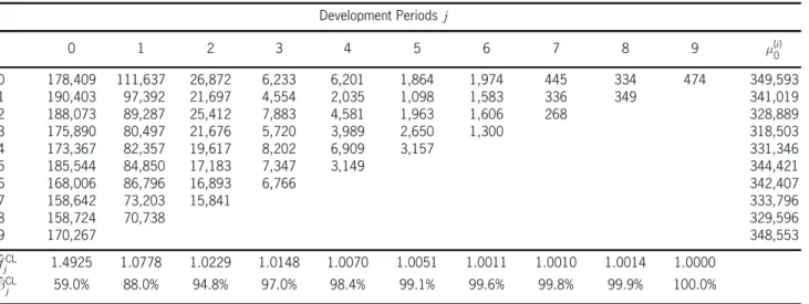
Table 1. Data and chain ladder parameter estimates

Development Periodsj

0 1 2 3 4 5 6 7 8 9 ¹(i)

0

0 178,409 111,637 26,872 6,233 6,201 1,864 1,974 445 334 474 349,593 1 190,403 97,392 21,697 4,554 2,035 1,098 1,583 336 349 341,019 2 188,073 89,287 25,412 7,883 4,581 1,963 1,606 268 328,889 3 175,890 80,497 21,676 5,720 3,989 2,650 1,300 318,503 4 173,367 82,357 19,617 8,202 6,909 3,157 331,346 5 185,544 84,850 17,183 7,347 3,149 344,421

6 168,006 86,796 16,893 6,766 342,407

7 158,642 73,203 15,841 333,796

8 158,724 70,738 329,596

9 170,267 348,553

ˆ

f_jCL 1.4925 1.0778 1.0229 1.0148 1.0070 1.0051 1.0011 1.0010 1.0014 1.0000 ˆ

¯_jCL 59.0% 88.0% 94.8% 97.0% 98.4% 99.1% 99.6% 99.8% 99.9% 100.0%

is an unbiased estimator for ¿2 (see [5] (4.26)). Since f¿2 _{could be negative, we set}

c

¿2_{= maxf¿}f2_{, 0g and ·b}

i=¾c2¢(¹ (i) 0 )¡

2_=¿c2_:

(4.11)

REMARK One may view as a major deficiency

of the present model that we lose the optimali-ties when replacing the unknown parameters by their estimates. On the other hand the following formula shows that it can be very useful in prac-tice: define ®(j)_i,¤ = ˆ¯_jCL=( ˆ¯_jCL+·b_i). For I_¡i < J, equation (2.14) leads to the following estimate of the ultimate claim payments:

f

Ci,J

¤

=Ci,I_¡i+ (1¡¯ˆICL_¡i)¢

Ã

®(iI,¤¡i)¢

C_i,I¡i

ˆ

¯CL

I¡i

+ (1¡®(i,I¤¡i))¢¹

(i) 0

!

=®(i,I¤¡i)¢Cci,J

CL

+ (1¡®i(,I¤¡i))¢Cci,J

BF

: (4.12)

In the last step above we have assumed that both

f_j and ¯_j are estimated by (4.1) (this is the usual choice done in practice for the CL and the BF methods).

REMARKS

² Our estimateCg_i,J¤ for the ultimate claim pay-ments is a credibility weighted average of the CL estimate and the BF estimate. The credibil-ity weight is determined by the development pattern ¯_j, the a priori estimate ¹(i)₀ and the

variances ¾2 and ¿2 of the processes. Since it is increasing in ¯_j we give higher credibility to the CL estimate for older accident years.

² Combining the CL estimate and the BF esti-mate is a very old problem in claims reserving. In some insurance companies there are rules of thumb for when to choose which estimate (see also Mack [15]). Equation (4.12) gives a natural way to combine the CL and the BF es-timates.

4.1. Example

The observed incremental paymentsX_i,j,i,j₂ f0,: : :, 9g, are given in Table 1.

This is a rather homogeneous data set, with fast development. After two years, almost 90% of the total claim amount is paid. On the other hand it also looks long-tailed since we still observe some payments after seven years (in the present work we do not bother about choosing tail factors for the CL method).

Using our parameter estimates from above we obtain the following estimates for¾2 and ¿2

c

¾2_{= (10,119)}2

and ¿c2_{= (60)}2_:

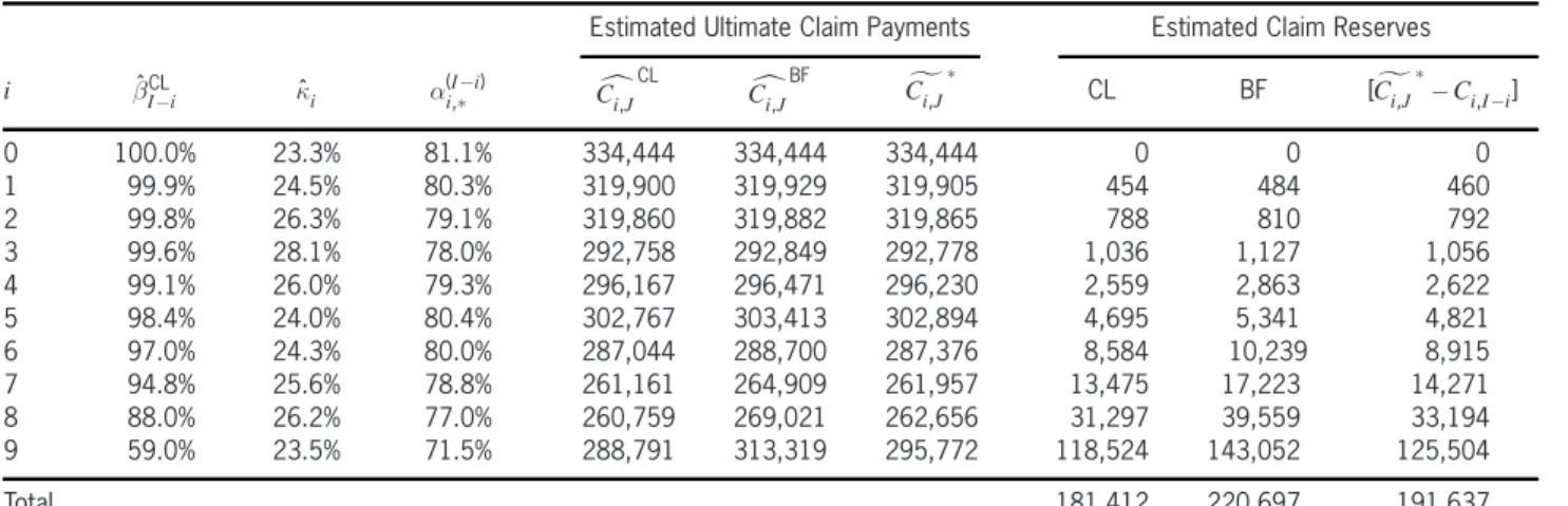
Table 2. Resulting reserves

Estimated Ultimate Claim Payments Estimated Claim Reserves

i ¯ˆCL_I¡i ·ˆ_i ®_i(I_,¤¡i) Cc_i,JCL Cc_i,JBF Cf_i,J¤ CL BF [Cf_i,J¤¡C_i,I¡i] 0 100.0% 23.3% 81.1% 334,444 334,444 334,444 0 0 0 1 99.9% 24.5% 80.3% 319,900 319,929 319,905 454 484 460 2 99.8% 26.3% 79.1% 319,860 319,882 319,865 788 810 792 3 99.6% 28.1% 78.0% 292,758 292,849 292,778 1,036 1,127 1,056 4 99.1% 26.0% 79.3% 296,167 296,471 296,230 2,559 2,863 2,622 5 98.4% 24.0% 80.4% 302,767 303,413 302,894 4,695 5,341 4,821 6 97.0% 24.3% 80.0% 287,044 288,700 287,376 8,584 10,239 8,915 7 94.8% 25.6% 78.8% 261,161 264,909 261,957 13,475 17,223 14,271 8 88.0% 26.2% 77.0% 260,759 269,021 262,656 31,297 39,559 33,194 9 59.0% 23.5% 71.5% 288,791 313,319 295,772 118,524 143,052 125,504

Total 181,412 220,697 191,637

Conclusions of the example.

² We see that the estimated ˆ·_i= (¾c2_=(¹(i) 0 )

2_)¢

(¿c2₎¡1 _{is around 25% in our example. This}

means that a claims development factor ˆ¯CL j

of 25% gives already a credibility weight of 50% to the observation. Observe also that the credibility weight is always smaller than 1.

² The a priori estimate ¹(i)₀ is rather conserva-tive since the BF estimate is always larger than the CL estimate. Of course, this can have var-ious reasons, which are not further discussed here. Our estimate Cg_i,J¤ then lies between the CL and the BF estimates. Since the credibility weights ®(I_i,¤¡i) are larger than 50%, our esti-mate is closer to the CL estiesti-mate.

References

[1] Benktander, G., “An Approach to Credibility in Cal-culating IBNR for Casualty Excess Reinsurance,” Actuarial Review, April 1976, p. 7.

[2] Bernardo, J. M., and A. F. M. Smith,Bayesian The-ory, New York: Wiley, 1994.

[3] Bornhuetter, R. L., and R. E. Ferguson, “The Actu-ary and IBNR,”Proceedings of the Casualty Actuar-ial Society59, 1972, pp. 181—195.

[4] Buchwalder, M., H. B¨uhlmann, M. Merz, and M. V. W¨uthrich, “The Mean Square Error of Predic-tion in the Chain Ladder Reserving Method (Mack and Murphy revisited),” ASTIN Bulletin 36, 2006, pp. 521—571.

[5] B¨uhlmann, H., and A. Gisler,A Course in Credibil-ity Theory and Its Applications, New York: Springer, 2005.

[6] de Alba, E., “Bayesian Estimation of Outstanding Claim Reserves,”North American Actuarial Journal 6:4, 2002, pp. 1—20.

[7] de Alba, E., “Claims Reserving When There Are Negative Values in the Runoff Triangle: Bayesian Analysis Using the Three-Parameter Log-Normal Distribution,” North American Actuarial Journal 10:3, 2006, pp. 45—59.

[8] de Alba, E., and M. A. Ramírez Corzo, “Bayesian Claims Reserving When There Are Negative Val-ues in the Runoff Triangle,”2006.1 Proceedings of Instituto Tecnol´ogico Aut´onomo de M´exico, Actuarial Research Clearing House, 2006, http://www.soa.org/ news-and-publications/files/pdf/arch06v40n1 VII. pdf.

[9] De Vylder, F., “Estimation of IBNR Claims by Cred-ibility Theory,” Insurance: Mathematics and Econ-omics1, 1982, pp. 35—40.

[10] England, P. D., and R. J. Verrall, “Stochastic Claims Reserving in General Insurance,” British Actuarial Journal8, 2002, pp. 443—518.

[11] Haastrup, S., and E. Arjas, “Claims Reserving in Continuous Time: A Nonparametric Bayesian Ap-proach,”ASTIN Bulletin26, 1996, pp. 139—164.

[12] Hovinen, E., “Additive and Continuous IBNR,” ASTIN Colloquium, Loen, Norway, 1981.

[13] Mack, T., “Improved Estimation of IBNR Claims by Credibility,”Insurance: Mathematics and Economics 9, 1990, pp. 51—57.

[14] Mack, T., “Distribution-Free Calculation of the Stan-dard Error of Chain Ladder Reserve Estimates,” ASTIN Bulletin23, 1993, pp. 213—225.

[16] McCullagh, P., and J. A. Nelder,Generalized Linear Models (2nd edition), London: Chapman and Hall, 1989.

[17] Neuhaus, W., “Another Pragmatic Loss Reserving Method or Bornhuetter/Ferguson Revisited,” Scan-dinavian Actuarial Journal, 1992, pp. 151—162. [18] Ntzoufras, I., and P. Dellaportas, “Bayesian

Mod-elling of Outstanding Liabilities Incorporating Claim Count Uncertainty,”North American Actuarial Jour-nal6:1, 2002, pp. 113—128.

[19] Scollnik, D. P. M., “Implementation of Four Models for Outstanding Liabilities in WinBUGS: A

Discus-sion of a Paper by Ntzoufras and Dellaportas,”North American Actuarial Journal6:1, 2002, pp. 113—128. [20] Verrall, R. J., “Bayesian and Empirical Bayes Esti-mation for the Chain Ladder Model,”ASTIN Bulletin 20, 1990, pp. 217—238.

[21] Verrall, R. J., “An Investigation into Stochastic Claims Reserving Models and Chain-Ladder Tech-nique,” Insurance: Mathematics and Economics 26, 2000, pp. 91—99.