Available online throug
ISSN 2229 – 5046
A WALD TEST FOR OVER DISPERSION IN ZERO-INFLATED POISSON REGRESSION MODEL
CH. SREELATHA*
1AND Dr. B. MUNISWAMY
21,2
Department of statistics, Andhra University, Visakhapatnam-530003, India.
(Received On: 20-04-18; Revised & Accepted On: 26-05-18)
ABSTRACT
W
e have considered the regression models to fit the count data especially in the field of Biometrical, Environmental, Social Sciences, and Economical areas. In the field of medical applications the count data with extra zeros are also common. The zero-inflated Poisson (ZIP) regression model is helpful to examine such data. Here we awareness on the use of ZIP model for analysis of count data including maximum likelihood estimation for regression coefficients using Fisher scoring method, compare between Poisson and ZIP models by various tests: likelihood ratio test, score test, chi-square test, test based on a confidence interval test and Cochran test. Model selection using Deviance method, AIC and BIC. We can find a Wald test for ZIP model in a single sample case for detecting zero-inflation in Poisson model and conduct a small simulation study in order to investigate sampling distribution of Wald test and power of Wald test. From our study we found that distribution can be used to detect the zero-inflation in counts.Keywords: Count data, Poisson model, Zero-inflated Poisson, Fisher Scoring Method, Wald test, AIC, BIC.
1. INTRODUCTION
In many medical applications, counts of events occurring in a given time or exposure period are discrete random variable having Poisson distribution. Based on the basic concept of generalized linear models (glms), the relationship between explanatory variables and response variable of Poisson counts can be described by Poisson regression or log linear models. The Poisson model is formed under two principal assumptions: one is that events occur independently over given time or exposure period and the other is that the conditional mean and variance are equal. However, in practice, the equality of the mean and variance rarely occurs; the variance may be either greater or less than the mean. If the variance is greater than the mean, it means that counts are more variable than specified by the Poisson events and are describe as overdispersion. If the variance is less than the mean, it means that counts are less variable than specified by the Poisson events and are describe as underdispersion. However, in practice, underdispersion is less common (McCullagh and Nelder, 1989). Moreover, overdispersion can be caused by excess number of observed zero counts, since the excess zeros will give smaller conditional mean than the true value. The count data with excess zeros, is known as zero-inflated Poisson counts. Of course it is possible to have fewer zero counts than expected, but this is less common in practice (Ritout et al., 1998). The count data encountered contain excess zeros relative to the Poisson distribution. A popular approach to analyse such data is to use a zero-inflated Poisson (ZIP) regression model. The ZIP model combines the Poisson distribution with a degenerate component of point mass at zero. A review of the ZIP methodology can be found in References Often the outcome of interest in public health and medical studies is a count
variable, which is usually assumed to follow the Poisson distribution and can be modeled accordingly. However, the
count variable may contain excess zeroes above what is to be expected from the Poisson model. These excess zeroes may be due to 1) the presence of a subpopulation with only zero counts, 2) overdispersion, or 3) chance (Campbell, Machin, and D’Arcangues, 1991). A common approach for analyzing such data is the zero-inflated Poisson (ZIP) model (Mullahy, 1986; Lambert, 1992), which is an extension of Cohen’s (1960) modified Poisson distribution. ZIP modeling has been used to analyze data on caries prevention (Bohning, Dietz, Schlattmann, Mendonca, and Kirchner, 1999), early growth failure in children (Cheung, 2002), and sudden infant death syndrome (Dalrymple, Hudson, and Ford, 2003), as well as many other diseases. ZIP modeling also can accommodate the extent of individual exposure (Lee, Wang, and Yau, 2001). ZIP models also have been extended to the bivariate (Walhin, 2001) and multivariate settings (Li, Lu, Park, Brinkley, and Peterson, 1999). Hall (2000) and Yau and Lee (2001) have used random-effects
approaches to extend the ZIP model to analyze longitudinal count data.This paper will be focussed only on ZIP models
and will proposed a Wald test for comparing between the standard Poisson and ZIP models.
Corresponding Author:
Ch. Sreelatha*
1,
© 2018, IJMA. All Rights Reserved 202 2. POISSON REGRESSION MODEL
Poisson regression model provide a standard framework for the analysis of count data. Suppose we have an independent sample on n pairs of observations (𝑦𝑖,𝑥𝑖)𝑖∈1,2,….𝑛,where yi denotes the number of times an event has
occurred and xi is the value of the explanatory variable for the ith subject. Assume 𝑦𝑖~𝑃𝑜𝑖𝑠𝑠𝑜𝑛(𝜆𝑖) then the probability
density function of Poisson random variables, yi, is given by
( ; )
,
0,1, 2,....
!
y
e
f y
y
y
λλ
λ
=
−=
Where λ>0, represents the expected number of occurrences in a fixed period of time. The mean and variance of the Poisson regression model is give as follows:
Figure2.1 : Poisson distribution plot with different means
Figures-2.1: illustrated four characteristics of the Poisson distribution that are important to understand the regression models for count dataset. Then we have the following empirical observations.
1. As λ increases, the curve of the distribution shifts to the right, where is the mean of the distribution.
2. Var(y) = λ, which is known as equi-dispersion. In real data, many count variables have a variance greater than the mean, which is called Overdispersion.
3. As λ increases, the probability of a zero count decreases. For many count dataset, there are more observed zeros than predicted by the Poisson distribution.
4. As λ increases, the Poisson distribution approximates a normal distribution. This is shown by the distribution for λ=10.
Let x be n×p matrix of explanatory variables. The relationship between yiand ithrow vector of x, xi, linked by g(λi) is
given by:
log( )
T,
1, 2,...,
i
x
ii
p
λ
=
β
=
This model is known as the Poisson regression model or log-linear model. To find the maximum likelihood function of
λi, we define the likelihood function as fallows:
1 1
(
)
( , )
!
!
T
xi T
i yi e xi yi
n n
i i
i i i i
e
e
e
L
l
y
y
β
λ
λ
βλ β
− −= =
=
=
∏
=
∏
Taking log on both sides and we get:
[
]
1 1
log( ( , ))
log
log
!
iTlog
!
n n
x T
i i i i i i i i
i i
L
l
λ β
y
λ λ
y
y x
β
e
βy
= =
A Wald test for over dispersion in zero-inflated Poisson regression model / IJMA- 9(6), June-2018.
The first derivative of the log likelihood function is
1
exp(
)
n
T
i i ij
i j
L
y
x
β
x
β
=∂
=
−
∂
∑
The second derivative of the log likelihood function is 2
exp(
iT)
ij ikj k
L
x
β
x x
β β
∂
= −
∂ ∂
∑
Hence, the log-likelihood function of the Poisson regression model is nonlinear in β so that they can be obtained via using an iterative algorithm. The most commonly used iterative algorithms are either Newton-Raphson or Fisher scoring. In practice 𝛽�is the solution of the estimating equations obtained by differentiating the log likelihood, (2) in
terms of β and equating them to zero. Therefore, β will be obtained by maximizing using numerical iterative method (McCullagh and Nelder, 1989).
3. ZERO-INFLATED POISSON REGRESSION MODEL
The zero-inflated Poisson model is a simple mixture model for count data with excess zeros, discovered by Lambert (1992). The model is a combination of a Poisson distribution and a degenerate distribution at zero. Specifically, if Yi
are independent random variables having a Zero-inflated Poisson distribution, the zeros are assumed to arise in two
ways corresponding to distinct underlying states. The first state occurs with probability πi and produces only zeros,
while the other state occurs with probability 1- πi and leads to a standard Poisson count with mean λi and hence a
chance of further zeros. In general, the zeros from the first state are called structural zeros and those from the Poisson distribution are called sampling zeros. This two-state process gives a simple two-component mixture distribution with probability mass function.
(1
) exp(
),
0
(
|
,
)
exp(
)
(1
)
,
1, 2, ,..., 0
1
!
i i i i
yi
i i i i i
i i i
i
y
P y
y
y
π
π
µ
π µ
π
µ µ
π
+ −
−
=
=
−
−
=
≤
≤
(3.1)
Which we denote by
Y
i~
ZIP
( ,
µ π
i i).
The mean and variance of Yi are(
|
,
)
(1
)
zip i i i i i
E
y
π µ
= −
π µ
,and
(
|
,
)
(
|
,
)(1
)
zip i i i zip i i i i i
Var
y
π µ
=
E
y
π µ
+
π µ
For a random sample of observations y1,y2,….,yn , the log-likelihood function is given by
{
( 0) ( 0)}
1
( , ; )
ln[
(1
)
i]
[ln(1
)
ln
ln( !)]
i i
n
i i y i i i i i y
i
y
e
µI
y
y
I
µ π
π
π
−π
µ
µ
= >
=
=
=
∑
+ −
+
−
−
+
−
(3.2)Where I(.) is the indicator function for the specified event, i.e. equal to 1 if the event is true and 0 otherwise. To apply the zero-inflated Poisson model in practical modeling situations, Lambert(1992) suggested the fallowing joint models for µi and πi
ln(
)
ln
,
1, 2,...,
1
T i T
i i i
i
x
and
π
z
i
n
µ
β
γ
π
=
=
=
−
(3.3)Where, xi and ziare covariate matrices and β,γ are (p+1)×1 and (q+1)×1 vector of unknown parameters, respectively.
Note that the vector of covariates xi and zi can be the same or different.
Clearly, the ZIP distribution, reduces to the Poisson distribution, when πi=0 . However, πi =0 is not valid in the logit
link function. Other link functions can be specified for either µiand πi. while the logit link for πi may seem the natural
choice, fallowing the description given in Jansakul and Hinde (2002), it is useful to use the identity link giving the joint models
ln(
µ
i)
=
x
iTβ
and
π
i=
z
iTγ
.
(3.4)© 2018, IJMA. All Rights Reserved 204 3.1: Maximum likelihood estimation for ZIP regression models
Based on the ZIP model (3.1), the log-likelihood function(3.2) and the model for µ and π displayed in (3.4), it is obvious that being a finite mixture the ZIP distribution is not a member of exponential family distribution and so standard GLM fitting procedures will not be adequate. To obtain the parameter estimates of ZIP regression models,
ˆ
and
ˆ
β
γ
, the Newton –Raphson method or the method of Fisher scoring can be used. However, the method of scoring is more appropriate for ZIP regression because the second derivativel
( , ; )
µ π
y
can be simplified by taking expectations.3.2 The Method Of Fisher Scoring
Assuming that µ and π in (3.4) are not functionally related. The first and second derivatives of l with respect to β and γ
are
(
,
)
ij i j
µ π
µ
β
µ
β
∂
∂
∂
=
∂
∂
∂
( )
[
]
( 0) 0 ,
1
(1
)
1, 2,.... ;
(1
)
i
i i i
n
i i
y y i i ij
i i i
e
I
I
y
x j
p
e
µµ
π µ
µ
π
π
−
= − >
=
− −
=
+
−
=
+ −
∑
(3.5)
(
,
)
ir i r
µ π
π
γ
π
γ
∂
∂
∂
=
∂
∂
∂
(
)
( )( 0) 0 ,
1
1
1
1, 2,...., ;
1
1
i
i i i
n
y y ir
i i i i
e
I
I
z
r
q
e
µµ
π
π
π
−
= − >
=
−
=
−
=
+ −
−
∑
(3.6)
and(
)
(
)
(
)
( )[ ]
2( 0) 2 0
1
1
[(1
)
1
]
,
,
1, 2,...., ;
1
i i
i i
i
n
i i i i i
y y i ij ik
i
j k i i
e
e
I
I
x x
j k
p
e
µ µ
µ
π µ
µ π
π
µ
β β
π
π
− − = > =
− −
−
+ −
∂
=
+
−
=
∂ ∂
+ −
∑
(3.7){
2 2( 0) 2 ( 0) 2
1
(1
)
1
}
, ,
1, 2,.... ;
[
(1
)
]
(1
)
i
i i i
n
y y ir is
i
r s i i i
e
I
I
z z
r s
q
e
µµ
γ γ
π
π
π
−
= − >
=
∂
=
− −
−
=
∂ ∂
∑
+ −
−
(3.8)2 2
( 0) 2 .
1
[
(1
)
]
i
i i
n
y ij ir
i
j r s j i i
e
I
x z
e
µ µ
µ
β γ
γ β
π
π
− = − =
∂
=
∂
=
∂ ∂
∂ ∂
+ −
∑
(3.9)Using the fact that
( 0)
( 0)
[
]
(
0)
(1
)
[
]
(
0) (1
)(1
)
i
i
i
i
y i i i
y i i
E I
P Y
e
and
E I
P Y
e
µ µ
π
π
π
− = − >=
= = + −
=
> = −
−
(
) (
)
(
)
(
)
2 , 11
1
1
(1
)
(1
)
1
i i
i i
n
i i i i i
i ij ik
i
j k i i
e
e
E
e
x x
e
µ µ
µ µ
π µ
µ π
π
π µ
β β
π
π
− − − − =
−
−
+ −
∂
−
∂ ∂
=
+ −
+ −
−
∑
(3.10) 2 2 , 1(1
)
1
(1
)
1
i i
i
n
ir is i
r s i i i
e
e
E
z z
e
µ µ
µ
γ γ
π
π
π
A Wald test for over dispersion in zero-inflated Poisson regression model / IJMA- 9(6), June-2018. and
(
)
2 11
i i n i ij ir ij r i i
e
E
x z
e
µµ
µ
β γ
π
π
− − =
∂
−
−
∂ ∂
=
+ −
∑
(3.12)Hence the estimates of β and γ at the (m+1)th iteration, denotes by β(m+1)and γ(m+1), are given by
( 1) ( )
1
( ) ( )
( 1) ( )
( , )
( , ),
m m
m m
m m
I
S
β
β
β γ
β γ
γ
γ
+ − +
=
+
Where the score vector and the expected information matrix, respectively evaluated at β= β(m+1) and γ =γ(m+1) are as
fallows.
( , )
( , )
( , )
( , )
( , )
S
S
S
β γµ π
β γ
β
β γ
β γ
µ π
γ
∂
∂
=
=
∂
∂
And the expected information matrix
I
( , )
β γ
( , )
( , )
( , )
,
( , )
( , )
I
I
I
I
I
ββ βγ γβ γγβ γ
β γ
β γ
β γ
β γ
=
(3.14)Where the elements
I
ββ,I
βγ=
I
γβTand I are respectively
γγ,
,
2 2 2
( , )
( , )
( , )
,
,
.
T T
E
µ π
E
µ π
and E
µ π
β β
β γ
γ γ
∂
∂
∂
−
−
−
∂ ∂
∂ ∂
∂ ∂
Denote the inverted expected Fisher information matrix
I
(
β γ
,
)
asK
(
β γ
,
)
,
( , )
( , )
( , )
( , )
( , )
( , )
( , )
( , )
( , )
I
I
K
K
K
I
I
K
K
ββ βγ ββ βγ
γβ γγ γβ γγ
β γ
β γ
β γ
β γ
β γ
β γ
β γ
β γ
β γ
=
=
(3.15)Note that Var(
β
ˆ
)
and Var
( )
γ
ˆ
are obtained fromI
−1( , ),
β γ
in
(3.13)
using inverse of partitioned matrix (Searle,1996) as follow1 1
ˆ
( )
( , )
( , )
( , )
( , )
K
ββ=
Var
β
=
I
βββ γ
−
I
βγβ γ
I
γγ−β γ
I
γββ γ
− (3.16)1 1
ˆ
( )
( , )
( , )
( , )
( , )
K
γγ=
Var
γ
=
I
γγβ γ
−
I
γββ γ
I
ββ−β γ
I
βγβ γ
− (3.17) With good stating valuesβ
0and
γ
0and hence
µ π
(0),
(0) the iterative scheme converges in a few step, convergence is obtained with a stopping rule, such as
(m+1)−
m≤
e
,
where
(m+1)and
( )marethe
log
−
likelihood
, ( , ; )
µ π
y
evaluated using the estimates ofµ
and
π
from the m and m+1 iterations, respectively. The asymptotic variance-covariance matrix for( )
β γ
ˆ ˆ
,
is automatically provided at the final iteration.3.3.Maximum Likelihood Estimation for ZIP Models with no Covariates
Based on the log-likelihood function, the maximum likelihood estimates µ and π are the roots of the equations
( , )
( , )
0
and
0.
µ π
µ π
µ
π
∂
=
∂
=
∂
∂
here we have
(
)
(
)
(
)
(
)
1 0 1,
1
,
1
J j J j j jj
e
e
µ µη
µ π
η
π
η
µ
π
π
µ
− = − =
×
∂
−
−
=
−
+
∂
+ −
∑
∑
(3.12)and
(
)
(
)
( )
1 0
,
(1
)
,
1
1
J j je
e
µ µη
µ π
η
π
π
π
µ
© 2018, IJMA. All Rights Reserved 206
Setting each of these equal to zero gives
(
)
(
)
(
)
ˆ 1 0 ˆ 1ˆ
1
ˆ
ˆ
1
ˆ
J j J j j j
j
e
e
µ µη
η
π
η
µ
π
π
− = − =×
−
+
=
+ −
∑
∑
and(
)
(
)
(
1)
0
ˆ ˆ
ˆ
1
ˆ
1
ˆ
1
J
j j
e
µe
µη
η
π
π
π
= −−
=
+ −
−
∑
Substituting (3.15) in to (3.14) gives
(
)
(
)
ˆ 1 1 ˆ 1ˆ
1
n nj n j
j j j j
e
j
e
µ µη
η
η
µ
− = = − =×
+
=
−
∑
∑
∑
(
)
(
)
ˆ ˆ 1 ˆ 11
ˆ
1
n j n j j jj
e
e
e
µ µ µη
η
µ
− − = − =×
+ −
=
−
∑
∑
(
)
(
)
1 ˆ 1ˆ
1
n j j n j jj
e
µη
µ
η
= − =×
=
−
∑
∑
(
ˆ) (
)
1 1
1
ˆ
n j j n j je
µη
j
µ
η
− = =−
×
=
∑
∑
(3.16)Note that this does not depend on ω or,η0 from (3.15)
(
ˆ)
(
)
(
)
ˆ 01
ˆ
ˆ
ˆ
1
1
1
n
j j
e
µe
µη
−π
π
π
−η
=
−
−
=
+ −
∑
(
ˆ)
(
ˆ)
(
)
ˆ0 0
1 1
ˆ
ˆ
ˆ
1
1
1
n n
j j
j j
e
µe
µe
µη
−πη
−π η
π
−η
= =
−
−
−
=
∑
+ −
∑
(
) (
)
ˆ ˆ ˆ ˆ
0 0
1 1 1
ˆ
ˆ
ˆ
1
1
n n n
j j j
j j j
e
µe
µe
µe
µπ η π
−η πη
−η
− −η
= = =
−
+
−
=
−
−
∑
∑
∑
ˆ 0 0 1 ˆ 0 0 1 1ˆ
n j j n n j j j je
e
µ µη
η
η
π
η η
η η
A Wald test for over dispersion in zero-inflated Poisson regression model / IJMA- 9(6), June-2018.
4. TEST STATISTIC FOR ZERO-INFLATION PROPOSED IN ZIP MODELS
Within the family of regression models, testing if a regression models is adequate corresponding to testing
H
0:
π
=
0 ;
H
1:
π
>
0,
Here π is taken as constant.
There are a number of test statistics proposed for testing the hypothesis including Wald, score test, likelihood ratio test, chi-square test, test based on a confidence interval of probability zero-inflated counts and Cochran test. Most of the tests mentioned were derived based on a single homogeneous sample, i.e. µ and π are not depend upon covariates or constant. The expressions of the tests and their sampling distributions are summarized in following subsections.
4.1. Likelihood ratio test
Let
l
ˆ
rdenote the value of the log-likelihood function evaluated at the restricted maximum likelihood estimates (for instance, the Poisson model ), andl
ˆ
u the value of the log-likelihood function evaluated at the unrestricted maximum likelihood estimates (for instance, the zero-inflated Poisson modell), and the likelihood ratio test based on the ratio of two log-likelihood functions can be written asˆ
ˆ
2(
r u)
LRT
= −
l
−
l
ˆ ˆ
0
1 1
ˆ
2
{
ln( )
ln( )}
ln[
(1
)
]
ln (1
)
!
y
n J
i i i i y
i y
e
LRT
y
y
e
y
µµ
µ
λ
λ
η
π
π
−η
π
−= =
= −
− −
−
+ −
−
−
∑
∑
0
0 0
ˆ
ˆ
2
ln
(
) ln
(ln
1 ln )
ˆ
y
y
y
η
η
η η
µ
η
µ
η
µ
=
+
−
−
+
+ −
Where 𝑦� is the mean of the observations and 𝜇̂ is the estimated positive mean counts. This test statistic is approximately fallows chi-square distribution with one degree of freedom under the null hypothesis.
4.2. Score test
A score test for the hypothesis is proposed by Van den broek (1995). The test is derived based on the log-likelihood to
obtain the ratio of the score vector,
( , )
( , )
µ π
µ
µ π
π
∂
∂
∂
∂
and minus expected information,
2 2
2
2 2
2
( , )
( , )
,
0
( , )
( , )
E
E
evaluated at
E
E
µ π
µ π
µ
µ π
π
µ π
µ π
π µ
π
−
∂
−
∂
∂
∂ ∂
=
∂
∂
−
−
∂ ∂
∂
Or under H0 true. Using mathematical algebra, the score statistic is defined by
(
0)
0 0 00
2 ˆ 0
ˆ ˆ 2ˆ
,
(1
)
e
S
e
e
ye
µ
ω µ µ µ
η η
η
η
−
− − −
−
=
−
−
µ�𝑜 is the estimate of the Poisson parameter under the null hypothesis. This statistic will have an asymptotic chi-square
distribution with one degree of freedom under the null hypothesis.
4.3. Chi-square test
The chi-square statistic χ2is used to test if a sample of data came from a population with a specific distribution. The χ2 is commonly defined by
2 2
1
(
)
c
k k
k k
O
E
E
ω
χ
=
−
© 2018, IJMA. All Rights Reserved 208
Where c denotes the number of classes(categories) decided for a given data set, Ok and Ek are observed frequencies and
expected frequencies under the null hypothesis of the kth class, respectively. When the null hypothesis is valid,
χ
ω2 fallows an asymptotic chi-square distribution on (c-1) d.f.4.4. Test based on a confidence interval of probability zero-inflated counts
It is possible to derive a test based on asymptotic normality of the estimate of the parameters. Following the statistical properties of ZIP,
( )
( )
(1
)
E Y
=
E Y
= −
π µ λ
=
2
1
1 (1
)
( )
( )
.
1
Var Y
Var Y
n
n
π λ πλ
π
−
+
=
=
−
From the central limit theorem, the confidence interval can be written as
/ 2 / 2
(1
)
( )
Y
Z
Z
Var Y
α α
π µ
− −
−
≤
≤
/ 2
( )
(1
)
/ 2( )
Z
αVar Y
Y
π µ
Z
αVar Y
−
≤ − −
≤
2 2
/ 2 / 2
1 (1
)
1 (1
)
1
1
1
1
Y
Z
απ λ πλ
Y
Z
απ λ πλ
η
π
η
π
π
µ
µ
−
+
−
+
−
+
−
−
−
≤ ≤ −
/ 2
{
[
ˆ
]} /
/ 2{
[
ˆ
]} /
1
1
.
ˆ
ˆ
y
Z
αy
y
µ
y
η
y
Z
αy
y
µ
y
η
ω
µ
µ
−
+
−
+
+
−
−
≤ ≤ −
Hence, a test based on a positive one sided confidence interval of probability zero-inflated counts can be obtained as
ˆ
{
[
]} /
1
,
ˆ
y
Z
y
y
y
CI
ω αµ
η
µ
+
+
−
= −
Where µ� is the estimated positive mean counts under H1. The critical region of this test method is simply CIω > 0. That
is , when CIω > 0, we reject the null hypothesis at α level of significance and the ZIP model should be used instead of a Poisson models.
4.5. The Cochran test
This test is also known as C test. The C test is used to test the assumption of constant variance of the residuals in the analysis of variance. This test is a ratio that relates the largest empirical variance of a particular treatment to the sum of the variances of the remaining treatments. The C test statistic for ZIP model was developed by Xie et al. (2001) can be written as follows:
Here if one random variable
X
~
χ
12 thenX
~
N
(0,1)
. The Cochran test is transformed their original chi-square into its corresponding standard normal form. Cochran proposed to test any single deviation (s0-t0) when t is estimatedfrom the data
From 2
~
(0,1)
( )
( )
P
P
C
N
Var P
ωVar P
χ =
⇒
=
Here
P
=
η η
0−
e
−yVar P
( )
=
Var
(
η η
0−
e
−y)
0 1/ 2
(
)
[
(1
]
y
y y y
e
C
e
e
ye
ω
η η
η
−
− − −
−
=
−
−
Under the null hypothesis, the test statistic Cω is approximately normally distributed with zero mean and unit variance.
2
2
(
0)
[
(1
]
y
y y y
e
C
e
e
ye
ω
η η
η
−
− − −
−
=
−
−
A Wald test for over dispersion in zero-inflated Poisson regression model / IJMA- 9(6), June-2018.
4.6 Wald test
The Wald test is a statistical test, typically used to test whether an effect exists or not. A Wald test can be used in a great variety of different models including models for dichotomous or binary variables and models for continuous variables. Under the aspect of the Wald statistical test, named after Abraham Wald, in this paper we will develop a
Wald test for ZIP model with constant µ and π for testing the hypothesis
0
:
0 ;
1:
0,
H
π
=
H
π
>
Based on the basic idea of obtaining the Wald test is
2
ˆ
ˆ
( )
W
Var
ω
=
π
π
Where
π
ˆ
is the maximum likelihood estimate of ω under the ZIP model.ˆ 0 ˆ
(
)
ˆ
(1
)
e
e
µ µη η
π
η
− −−
=
−
1 1ˆ
( )
(
)
Var
π
=
I
ππ−
I I I
πµ µµ µπ− −Then
(
)
(
)
(
)
(
)
(
)
{
(
)
}
ˆ 2ˆ
1
ˆ ˆ ˆ ˆ
1
ˆ
ˆ
ˆ
ˆ
1
1
1
ˆ
ˆ
1
ˆ
ˆ
1
ˆ
ˆ ˆ
e
e
I
I I
I
e
e
e
e
µ µ
ππ πµ µµ µπ µ µ µ µ
µ
η
π π
π
π π
π
π
π
πµ
− − − − − − −
−
−
=
−
−
+ −
−
+ −
+ −
−
(
)
{
}
(
)
(
)
{
(
)
}
ˆ ˆ ˆ 2ˆ
ˆ ˆ ˆ
ˆ
ˆ
ˆ ˆ
ˆ
(1
)
1
ˆ
ˆ
ˆ
ˆ
ˆ
ˆ ˆ
1
1
1
e
e
e
e
e
e
e
µ µ µ µ
µ µ µ
η
π
π
πµ
µ
π π
π
π
π
πµ
− − − − − − −
−
+ −
−
=
−
+ −
+ −
−
(3.28) Since(
)
ˆ 0(
)
ˆ
1
ˆ
1
,
ˆ
y
e
µη
and
π
π
π
η
µ
−+ −
=
−
=
(3.28)(
)
(
)
{
}
(
)
(
)
ˆ ˆ ˆ
2 2
0 1
ˆ
0 0
ˆ
1
ˆ
ˆ
.
ˆ
e
y
e
e
I
I I
I
y
y
e
µ µ µ
ππ πµ µµ µπ µ
η µ
η
µ
η
ηµ
η
η
µ
η
− − − − −
−
−
−
−
−
=
−
−
(3.29)Hence
( )
(
)
(
)
(
)
(
)
{
}
ˆ
1 0 0
1
ˆ ˆ ˆ
2 2
0
ˆ
ˆ
ˆ
1
ˆ
ˆ
y
e
y
Var
I
I I
I
e
e
y
e
µ
ππ πµ µµ µπ µ µ µ
η
η η
µ
π
η µ
η η
µ
ηµ
− − − − − −
−
−
=
−
=
−
−
−
−
(3.30)The Wald test for ZIP model is given as
2 ˆ 0 ˆ ˆ 0 0
ˆ ˆ ˆ
2 2
0
ˆ 2 ˆ ˆ 2ˆ
0 0
ˆ 2 ˆ
0 0
(
)
(1
)
ˆ
[
(
)]
ˆ
{(1
)[
(
ˆ
)]
ˆ
}
ˆ
ˆ
ˆ
(
)
{(1
)[
(
)]
}
ˆ
(1
) [
(
)]
e
e
W
y
e
y
e
e
y
e
e
e
e
y
e
y
e
e
y
µ µ
ω µ
µ µ µ
µ µ µ µ
µ µ
η η
η
η η η
µ
η µ
η η
µ
ηµ
η η
µ
η η
µ
ηµ
η
η η
µ
− − − − − − − − − − − −
−
−
=
−
−
−
−
−
−
−
−
−
−
−
=
−
−
−
5. SIMULATION STUDY
© 2018, IJMA. All Rights Reserved 210
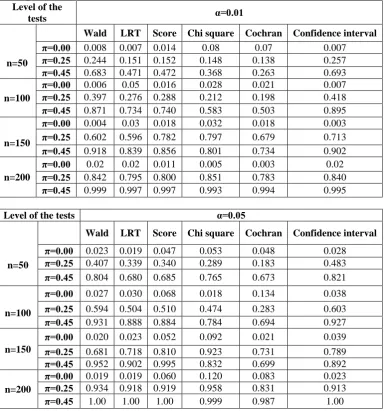
We can see that for a fixed value of π, the power of the those tests increases when sample size n increases. Similarly pattern is also found for increasing value of π and fixed n. here we can see the that when the value of π increases, number of excess zeros is large. The power of those tests are also good for this situation. For example when the sample
size is 200, and parameters are 2.00 and 0.45 for µ and π respectively, the powers are higher than 0.993. Additionally, these tests are all good for comparing between Poisson and ZIP models. It can it can be seen that wald test is good as the Cochran and confidence interval tests, but it is better than likelihood ratio test, score test and chi-square test. Thus, the Wald test can be an alternative test for comparing between Poisson and ZIP models.
Table-5.1: Power of Wald, LRT, Score, Chi-square, Cochran, Confidence interval test statistics without covariates based on 1000 samples from the ZIP model with at α=0.01, µ =2.00
Level of the
tests α=0.01
n=50
Wald LRT Score Chi square Cochran Confidence interval
π=0.00 0.008 0.007 0.014 0.08 0.07 0.007
π=0.25 0.244 0.151 0.152 0.148 0.138 0.257
π=0.45 0.683 0.471 0.472 0.368 0.263 0.693
n=100
π=0.00 0.006 0.05 0.016 0.028 0.021 0.007
π=0.25 0.397 0.276 0.288 0.212 0.198 0.418
π=0.45 0.871 0.734 0.740 0.583 0.503 0.895
n=150
π=0.00 0.004 0.03 0.018 0.032 0.018 0.003
π=0.25 0.602 0.596 0.782 0.797 0.679 0.713
π=0.45 0.918 0.839 0.856 0.801 0.734 0.902
n=200
π=0.00 0.02 0.02 0.011 0.005 0.003 0.02
π=0.25 0.842 0.795 0.800 0.851 0.783 0.840
π=0.45 0.999 0.997 0.997 0.993 0.994 0.995
Level of the tests α=0.05
n=50
Wald LRT Score Chi square Cochran Confidence interval
π=0.00 0.023 0.019 0.047 0.053 0.048 0.028
π=0.25 0.407 0.339 0.340 0.289 0.183 0.483
π=0.45 0.804 0.680 0.685 0.765 0.673 0.821
n=100
π=0.00 0.027 0.030 0.068 0.018 0.134 0.038
π=0.25 0.594 0.504 0.510 0.474 0.283 0.603
π=0.45 0.931 0.888 0.884 0.784 0.694 0.927
n=150
π=0.00 0.020 0.023 0.052 0.092 0.021 0.039
π=0.25 0.681 0.718 0.810 0.923 0.731 0.789
π=0.45 0.952 0.902 0.995 0.832 0.699 0.892
n=200
π=0.00 0.019 0.019 0.060 0.120 0.083 0.023
π=0.25 0.934 0.918 0.919 0.958 0.831 0.913
π=0.45 1.00 1.00 1.00 0.999 0.987 1.00
5.1 Example
A Wald test for over dispersion in zero-inflated Poisson regression model / IJMA- 9(6), June-2018.
Table-5.1: Observed and predicted probability from Poisson, ZIP model for the number of Road accidents death dataset
Count Frequency Observed probability Predicted probability Poisson ZIP
0 1005 0.6989 0.6951 0.6989
1 387 0.2691 0.2528 0.2462
2 30 0.0209 0.0460 0.0480
3 9 0.0063 0.0056 0.0063
4 4 0.0028 0.0005 0.0006
5 0 0.0000 0.0000 0.0000
6 0 0.0000 0.0000 0.0000
Table-5.2: Model selection criteria for Poisson and ZIP regression models for the number of Road accidents death dataset
Selection Criteria Models Poisson ZIP Log-likelihood 884.115 809.027
AIC 1794.230 1664.054
BIC 1862.753 1785.287
Figure-5.1: The Observed and predicted probability of Poisson and ZIP Models
6. DISCUSSION
Overdispersion is a common phenomenon in Poisson modeling, and this can be carried over to zero-inflated count data modeling. When zero-inflation exist in the count data, the ZIP model is frequently used. In this study, we have studied the properties of the score statistics, Cochran, Confidence interval, Chi-square, LRT, and Wald test statistics are examined via Monte Carlo simulations and application examples are given to illustrate our method.
© 2018, IJMA. All Rights Reserved 212 7. REFERENCES
1. Agresti A. (1996), An Introduction to Categorical Data Analysis, wiley.
2. Breslow, N. (1990). Tests of hypotheses in over-dispersed Poisson regression and other quasi- likelihood models. J. Amer. Statist. Assoc. 85, 565-571.
3. Cameron A.C. and Trivedi P.K. (1990). Regression Based Test for Overdispersion in the Poisson Model. Journal of Applied Econometrics, 46:347- 364.
4. Cameron A.C. and Trivedi P.K. (1998). Regression Analysis of Count Data. Cambridge University Press. 5. Dean, C. B. (1992). Testing for overdispersion in Poisson and binomial regression models, J. Amer. Statist.
Assoc. 87, 451-457.
6. Dejen Tesfaw.M and B.Muniswamy Power of Tests for Overdispersion Parameter in Negative Binomial Regression Model. IOSR Journal of Mathematics (IOSRJM) ISSN: 2278-5728 Volume 1, Issue 4 (July-Aug 2012), PP 29-36.
7. Jansakul, N. and Hinde, J. P. 2002. Score tests for zero-inflated Poisson models. Computational Statistics and Data Analysis. 40: 75-96.
8. Jansakul, N. and Hinde, J. P. 2009. Score tests for extra-zero models in zero inflated Negative Binomial models. Communications in statistics-simulation and computation. 38: 92-108.
9. Lambert, D. 1992. Zero-inflated Poisson regression with application to defects in manufacturing. Technometrics. 41(1): 29-38.
10. Mccullagh P. and Nelder J.A. (1989). Generalized Linear Models. Chapman and Hall, London.
11. Nelder, J. A. and Wedderburn, R. W. M. 1972. Generalized Linear Models. Journal of the Royal Statistical Society, Series A. 135(3): 370-384.
12. Ridout, M. S., Demetrio, C. G. B. and Hinde, J. P. 1998. Model for count data with many zeros. International Biometric Conference. 179-190.
13. Vuong Q.H. (1989). Likelihood ratio tests for model selection and non-nested hypotheses. Econometrica, 57:2:307-333.
Source of support: Nil, Conflict of interest: None Declared.