Vol 8, No 10 (2017)

(1)

Available online throug

ISSN 2229 – 5046

DIVISOR DEGREE ENERGY OF GRAPHS

S. P. KANNIGA DEVI

*

Department of Mathematics,

Kalasalingam Institute of Technology,

Anand Nagar, Krishnankoil-626 126,

Srivilliputhur(via), Virudhunagar - (Dist), Tamil Nadu, India.

K. NAGARAJAN

Department of Mathematics,

Kalasalingam University, Anand Nagar, Krishnankoil-626 126,

Srivilliputhur(via), Virudhunagar - (Dist), Tamil Nadu, India.

(Received On: 20-08-17; Revised & Accepted On: 23-09-17)

ABSTRACT

I

n this paper, we introduce the concepts of divisor degree matrix DD(G) of a simple graph G and obtain eigenvalues of DD(G). We also introduce divisor degree energy (DDE) of graphs denoted by EDD (G) and find DDE of some standard

graphs and also we establish the relation between energy and DDE of graphs.

Keywords: Energy, Divisor degree matrix, Divisor degree energy, Eigenvalues.

Mathematics Subject Classification: 05C50.

1. INTRODUCTION

In the study of spectral graph theory, we use the spectra of certain matrix associated with the graph, such as the adjacency matrix, the Laplacian matrix and other related matrices. Some useful information about the graph can be obtained from the spectra of these various matrices.

An adjacency matrix of G denoted by 𝐴=𝐴(𝐺) = [𝑎_𝑖𝑗] is a square matrix of order of n where

aij=�1, _0,𝑖𝑓𝑣𝑖𝑖𝑠𝑎𝑑𝑗𝑎𝑐𝑒𝑛𝑡_{𝑜𝑡ℎ𝑒𝑟𝑤𝑖𝑠𝑒}𝑡𝑜𝑣𝑗

The Characteristic polynomial |𝜆𝐼 − 𝐴| of A is called the characteristic polynomial of G and is denoted by

𝑃𝐺(𝜆) or 𝑃(𝐺) =

∑

= − n

i

i n i

a

1

λ

.

The eigenvalues of A, which are the zeros of |𝜆𝐼 − 𝐴| are the eigenvalues of G and form spectrum denoted by spec (G). If the distinct eigenvalues of G are 𝜆₁,𝜆₂, … ,𝜆_𝑛 with multiplicities 𝑡₁,𝑡₂, … ,𝑡_𝑛 respectively, then spec (G) is written as �𝜆1𝑡1,𝜆2𝑡2, … ,𝜆𝑛𝑡𝑛�. Since the adjacency matrix is a real symmetric matrix, all its eigenvalues are real and hence the

eigenvalues can be ordered as 𝜆₁≥ 𝜆₂≥ ⋯ ≥ 𝜆_𝑛.

Let G be a graph with 𝑠𝑝𝑒𝑐(𝐺) = {𝜆₁,𝜆₂, … ,𝜆_𝑛}. Then, the energy of G, denoted by E(G) is defined as

E(G) =

∑

= n

i i

1

λ

.

Leverrier’s Algorithm: This method allows us to find the characteristic polynomial of any 𝑛×𝑛 matrix A using the trace of the matrix AK, where 𝑘= 1,2, … ,𝑛. Let 𝜎(𝐴) = {𝜆₁,𝜆₂, … ,𝜆_𝑛} be the set of all eigenvalues of A which is also called the spectrum of A. Note that 𝑠_𝑘 =𝑡𝑟𝑎𝑐𝑒 (𝐴𝑘) =∑𝑛_𝑖=1𝜆𝑘_𝑖, for all 𝑘= 1,2, … ,𝑛.

(2)

𝑝𝑘 =−1_𝑘[𝑠𝑘+𝑝1𝑠𝑘−1+⋯+𝑝𝑘−1𝑠1] (𝑘= 1,2, … ,𝑛)

Various types of energies are studied in the mathematical literature [5]. Motivated by recent works on energy of a graph, in this paper we introduce divisor degree matrix associated with a graph and study its spectrum.

Let G be a simple graph with n vertices 𝑣₁,𝑣₂,𝑣₃, … ,𝑣_𝑛 and m edges. Let di be the degree of vi, 𝑖= 1,2, … ,𝑛. Define

𝑎𝑖𝑗 =

⎩ ⎪ ⎨ ⎪ ⎧ _�𝑑𝑖

𝑑𝑗�+�

𝑑𝑗

𝑑𝑖�, 𝑖𝑓𝑣𝑖𝑎𝑛𝑑𝑣𝑗𝑎𝑟𝑒𝑎𝑑𝑗𝑎𝑐𝑒𝑛𝑡

1, 𝑖𝑓𝑣𝑖𝑎𝑛𝑑𝑣𝑗𝑎𝑟𝑒𝑎𝑑𝑗𝑎𝑐𝑒𝑛𝑡𝑎𝑛𝑑𝑑𝑖=𝑑𝑗

0, 𝑜𝑡ℎ𝑒𝑟𝑤𝑖𝑠𝑒

where [x] denote integral part of real number x. Then the 𝑛×𝑛 matrix of G has its eigenvalues as 𝜆₁,𝜆₂, … ,𝜆_𝑛.

The divisor degree energy (DDE)of a graph is define as EDD(G) =

∑

= n

i i

1

λ

.

Since DD(G)is a symmetric matrix with zero trace, these divisor degree eigenvalues are real with sum equal to zero.

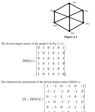
Example 1.1: Consider the graph G

Figure-1.1

The divisor degree matrix of the graph G in Fig 1.1 is













=

0

1

0

1

0

1

0

1

0

1

0

1

0

1

0

1

0

1

0

1

0

1

0

1

0

1

0

1

0

1

0 )

(

G

DD

The characteristic polynomial of the divisor degree matrix DD(G) is













−

=

−

λ

1

0

1

0

1

0

1

0

1

0

1

0

1

0

1

0

1

0

1

0

1 )

(

G

DD

I

(3)

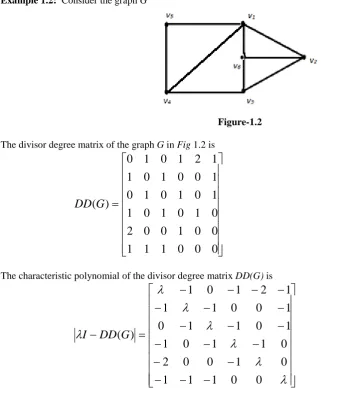
Example 1.2: Consider the graph G

Figure-1.2

The divisor degree matrix of the graph G in Fig 1.2 is













=

0

1

0

1

0

2

0

1

0

1

0

1

0

1

0

1

0

1

0

1

0

1

2

1

0

1

0 )

(

G

DD

The characteristic polynomial of the divisor degree matrix DD(G) is













−

=

−

λ

0

1

0

1

0

2

0

1

0

1

0

1

0

1

0

1

2

1

0

1 )

(

G

DD

I

From the Leverrier’s algorithm [4], it follows that 𝑃(𝐺) =𝜆6−12𝜆4−8𝜆3+ 23𝜆2+ 16𝜆 −4 and the divisor degree eigenvalues of G are 𝜆₁≅3.470,𝜆₂≅1.442,𝜆₃≅0.198,𝜆₄≅ −2.498,𝜆₅≅ −1.612,𝜆₆≅ −1. Thus,𝐸_𝐷𝐷(𝐺)≅ 10.22.

We now give the explicit expression for the coefficient 𝑎_𝑖 of 𝜆𝑛−𝑖 (𝑖= 0,1,2,3) in the characteristic polynomial of the divisor degree matrix DD(G). It is clear that 𝑎₀= 1 and 𝑎₁=𝑡𝑟𝑎𝑐𝑒𝐷𝐷(𝐺) = 0.

(i) We have

𝑎2= � �_𝑎0 𝑎𝑗𝑘

𝑘𝑗 0�

1≤𝑗<𝑘≤𝑛

But ��0 𝑎𝑗𝑘

𝑎𝑘𝑗 0�=�− �� 𝑑𝑗 𝑑𝑘�+�

𝑑𝑘 𝑑𝑗��

2

, 𝑣𝑗𝑎𝑛𝑑𝑣𝑘𝑎𝑟𝑒𝑎𝑑𝑗𝑎𝑐𝑒𝑛𝑡

0, 𝑜𝑡ℎ𝑒𝑟𝑤𝑖𝑠𝑒

Thus

𝑎2=−1₂� �� _𝑑𝑑𝑗 𝑘�+�

𝑑𝑘

𝑑𝑗�� 2

𝑗~𝑘

�

𝑛

𝑗=1

where ∑_𝑗_~_𝑘 indicates summation over all pair of adjacent vertices 𝑣_𝑗,𝑣_𝑘.

Example 1.3: For the graph G in Fig 1.2 the coefficient 𝑎₂ of 𝜆2 in the characteristic polynomial of the divisor degree matrix DD(G) is equal to

−1₂∑ �∑ ��𝑑𝑗 𝑑 �+�

𝑑𝑘 𝑑��

2

𝑗~𝑘 �

𝑛

𝑗=1 =−1₂�(1

2_{+ 2}2_{+ 1}2_{+ 1}2_{) + (1}2_{+ 1}2_{+ 1}2_{) + (1}2_{+ 1}2_{+ 1}2₎

(4)

𝑎3= (−1)3 � �

𝑎𝑖𝑖 𝑎𝑖𝑗 𝑎𝑖𝑘

𝑎𝑗𝑖 𝑎𝑗𝑗 𝑎𝑗𝑘

𝑎𝑘𝑖 𝑎𝑘𝑗 𝑎𝑘𝑘

�

1≤𝑖<𝑗<𝑘≤𝑛

𝑎3=−2 � 𝑎𝑖𝑗𝑎𝑗𝑘𝑎𝑘𝑖 ∆𝑣𝑖𝑣𝑗𝑣𝑘

where ∑_∆𝑣_𝑖_𝑣_𝑗_𝑣_𝑘 indicates summation over all pair of adjacent vertices𝑣_𝑖,𝑣_𝑗 and 𝑣_𝑘of triangles in a graph.

Remark 1.4:

a) Number of terms in the above sum is equal to the number of triangles in the graph. b) If there is no triangle in the graph G, then 𝑎₃= 0.

Example 1.5: For the graph G in Fig 1.2 the coefficient 𝑎₃ of 𝜆3 in the characteristic polynomial of the divisor degree matrix DD(G) is equal to

−2 ∑∆𝑣𝑖𝑣𝑗𝑣𝑘𝑎𝑖𝑗𝑎𝑗𝑘𝑎𝑘𝑖=−2�(1 × 1 × 1) + (1 × 1 × 1) + (1 × 1 × 2)�=−8 .

Theorem 1.6: If 𝜆₁,𝜆₂, … ,𝜆_𝑛 are the divisor degree eigenvalues of a graph G, then ∑𝑛𝑖=1𝜆𝑖2=−2𝑎2

Proof: We have

∑𝑛𝑖=1𝜆2𝑖 = 𝑡𝑟𝑎𝑐𝑒�𝐷𝐷(𝐺)�2=∑ �∑𝑖=1𝑛 𝑛𝑗=1𝑎𝑖𝑗𝑎𝑗𝑖� = ∑ �∑ ��_𝑑𝑑𝑖_𝑗�+�𝑑_𝑑𝑗_𝑖�� 2

𝑖~𝑗 �

𝑛

𝑖=1

= −2𝑎₂.

2. THE DIVISOR DEGREE ENERGY OF SOME STANDARD GRAPHS

We observe that the adjacent matrix of energy and divisor degree matrix of a regular graphs are same. So, DDE is equal to the energy of the regular graphs [8]. Hence, we have the following results.

Result 2.1:

i) 𝐸_𝐷𝐷(𝐾_𝒏) = 2(𝑛 −1) ii) 𝐸_𝐷𝐷�𝐾_𝑛_,_𝑛�= 2𝑛 iii) 𝑠𝑝𝑒𝑐 (𝐶_𝑛) = 2 cos�2𝜋𝑗

𝑛 � (𝑗= 0,1, … ,𝑛 −1).

Theorem 2.2: If G is a path Pn of order n, (𝑛 ≥ 𝑘+ 2), then

𝑃(𝑃𝑛) =𝜆𝑘+2−8𝜆𝑘+ 8𝑘 ∑ (−1) 𝑟 𝑟+1 �𝑘₂�−1

𝑟=0 �𝑘 − 𝑟 −_𝑟 2� 𝜆𝑘−2(𝑟+1)− ∑ (−1)𝑟 �𝑘₂�−1

𝑟=0 �𝑘 − 𝑟 −_𝑟_{+ 1}1� 𝜆𝑘−2𝑟,

𝑛 ≥ 𝑘+ 2,𝑘 ∈ 𝑁 . Proof: For 𝑛= 3,

𝐷𝐷(𝑃3) =�

0 2 0 2 0 2 0 2 0� |𝜆𝐼 − 𝐷𝐷(𝑃3)| =�

𝜆 −2 0 −2 𝜆 −2

0 −2 𝜆 �

From the Leverrier’s algorithm [4], it follows that 𝑃(𝑃₃) =𝜆3−8𝜆

Similarly, for 𝑛= 4,𝑃(𝑃₄) =𝜆4−9𝜆2+ 16 𝑛= 5,𝑃(𝑃₅) =𝜆5−10𝜆3+ 24𝜆 𝑛= 6,𝑃(𝑃₆) =𝜆6−11𝜆4+ 33𝜆2−16

𝑛= 7,𝑃(𝑃₇) =𝜆7−12𝜆5+ 43𝜆3−40𝜆 and so on.

(5)

The numbers in the row can be obtained by the following rule. The first number is 1 each and 16 is the last number in each odd rows except first row. The second number in each row is obtained by adding the previous row’s first number. The third number in each row is obtained by adding the previous second row’s second number and previous row’s third number. Likewise, the fourth number in each row is obtained by adding the previous second row’s third number and previous row’s fourth number and so on. This helps us to generalize the characteristic polynomial of a path Pn of order

n, 𝑛 ≥3,

𝑃(𝜆) =𝜆𝑛₋_{(8 +}_{𝑛 −}₃₎_𝜆𝑛−2₊_�₈₍_{𝑛 −}_{2) +}(𝑛−4)(𝑛−5)

2 � 𝜆𝑛−4− �

8(𝑛−2)(𝑛−5)

2 +

(𝑛−5)(𝑛−6)(𝑛−7)

3×2×1 � 𝜆𝑛−6

+�8(𝑛−2)(₃𝑛−6_×₂)(𝑛−7)+(𝑛−6)(𝑛−7₄_×)(₃_×𝑛−8₂ )(𝑛−9)� 𝜆𝑛−8 _{− ⋯}

=𝜆𝑘+2₋₈_𝜆𝑘₊_�₈_𝑘𝜆𝑘−2₋8𝑘(𝑘−3)

2 𝜆𝑘−4+

8𝑘(𝑘−4)(𝑘−5)

3×2 𝜆𝑘−6− ⋯ �

− �(𝑘−1₁ )𝜆𝑘₋(𝑘−2)(𝑘−3)

2 𝜆𝑘−2+

(𝑘−3)(𝑘−4)(𝑘−5)

3×2 𝜆𝑘−4− ⋯ �

where 𝑛 ≥ 𝑘+ 2,𝑘 ∈ 𝑁.

𝑃(𝑃𝑛) =𝜆𝑘+2−8𝜆𝑘+ 8𝑘 ∑ (−1) 𝑟 𝑟+1 �𝑘₂�−1

𝑟=0 �𝑘 − 𝑟 −_𝑟 2� 𝜆𝑘−2(𝑟+1)− ∑ (−1)𝑟 �𝑘₂�−1

𝑟=0 �𝑘 − 𝑟 −_𝑟_{+ 1}1� 𝜆𝑘−2𝑟,

𝑛 ≥ 𝑘+ 2,𝑘 ∈ 𝑁 .

Lemma 2.3 [2]: If M is a non singular square matrix then we have�𝑀 𝑁

𝑃 𝑄�= |𝑀||𝑄 − 𝑃𝑀−1𝑁|.

Theorem 2.4: If G is a complete bipartite graph 𝐾_𝑛₁_,_𝑛₂, then 𝑃�𝐾_𝑛₁_,_𝑛₂�=𝜆𝑛1+𝑛2−2₍_𝜆2_{− 𝑛}₁_𝑛₂_𝑘2₎_where_𝑛₂₌_𝑛₁_𝑘₊_𝑟_,

(0≤ 𝑟 ≤ 𝑛1−1) and 𝑘=�_𝑛𝑛2₁� is the integral part of real number 𝑛_𝑛2₁, (𝑛1≤ 𝑛2) and 𝐸𝐷𝐷�𝐾𝑛1,𝑛2�= 2𝑘√𝑛1𝑛2 .

Proof: Without loss of generality we partition the vertex set of the complete bipartite graph 𝐾_𝑛₁_,_𝑛₂ into disjoint sets 𝐴=�𝑢1,𝑢2, … ,𝑢𝑛1� and 𝐵=�𝑣1,𝑣2, … ,𝑣𝑛2� such that no two vertices in either sets are adjacent to each other. Then

the characteristic polynomial of 𝐾_𝑛₁_,_𝑛₂ is

�𝜆𝐼 − 𝐷𝐷�𝐾𝑛1,𝑛2��

λ

0

0 



k

−

=

T

N

I

λ

(6)













−

=

k

N



is a matrix of order 𝑛₂×𝑛₁ and 𝑁𝑇 is the transpose of 𝑁 of order

𝑛1×𝑛2 .

Applying lemma 2.3 to the expression (1), we get �𝜆𝐼 − 𝐷𝐷�𝐾𝑛1,𝑛2��=𝜆𝑛1�𝜆𝐼𝑛2− 𝑁

𝐼_𝑛1

𝜆 𝑁𝑇�=𝜆𝑛1−𝑛2�𝜆2𝐼𝑛2− 𝑁𝑁𝑇� (2)

Now,













=

2 1 2 1 2 1 2 1 2 1 2 1 2 1 2 1 2 1 2 1 2 1 2 1 2 1 2 1 2 1 2 1

k

n

k

n

k

n

k

n

k

n

k

n

k

n

k

n

k

n

k

n

k

n

k

n

k

n

k

n

k

n

k

n

NN

T



is a square matrix of order 𝑛₂.

Substituting

NN

Tin (2), we get

�𝜆𝐼 − 𝐷𝐷�𝐾𝑛1,𝑛2��=𝜆𝑛1−𝑛2_�

� 𝜆2_{− 𝑛}

1𝑘2 −𝑛1𝑘2 ⋯ −𝑛1𝑘2 −𝑛1𝑘2

−𝑛1𝑘2 𝜆2− 𝑛1𝑘2 ⋯ −𝑛1𝑘2 −𝑛1𝑘2

⋯ ⋯ ⋯ ⋯ ⋯

−𝑛1𝑘2 −𝑛1𝑘2 ⋯ 𝜆2− 𝑛1𝑘2 −𝑛1𝑘2

−𝑛1𝑘2 −𝑛1𝑘2 ⋯ −𝑛1𝑘2 𝜆2− 𝑛1𝑘2

�

�₍₃₎

Subtract row 𝑛₂ from the rows 1,2, … ,𝑛₂−1 of (3), we get

=𝜆𝑛1−𝑛2

� �

𝜆2 ₀ _⋯ ₀ _−𝜆2

0 𝜆2 _⋯ ₀ _−𝜆2

⋯ ⋯ ⋯ ⋯ ⋯

0 0 ⋯ 𝜆2 _−𝜆2

−𝑛1𝑘2 −𝑛1𝑘2 ⋯ −𝑛1𝑘2 𝜆2− 𝑛1𝑘2

� �

=𝜆𝑛1−𝑛2₍_𝜆2₎𝑛2−1

� �

1 0 ⋯ 0 −1

0 1 ⋯ 0 −1

⋯ ⋯ ⋯ ⋯ ⋯

0 0 ⋯ 1 −1

−𝑛1𝑘2 −𝑛1𝑘2 ⋯ −𝑛1𝑘2 𝜆2− 𝑛1𝑘2

� �

Thus, 𝑃�𝐾_𝑛₁_,_𝑛₂�=𝜆𝑛1+𝑛2−2(_𝜆2_{− 𝑛}₁_𝑛₂_𝑘2)_{, where}_𝑛₂₌_𝑛₁_𝑘₊_𝑟_{, (0}_{≤ 𝑟 ≤ 𝑛}₁₋₁₎_and_𝐸_𝐷𝐷_�𝐾_𝑛

1,𝑛2�= 2𝑘√𝑛1𝑛2.

Corollary 2.5: For a star 𝐾₁_,_𝑛₂,𝐸_𝐷𝐷�𝐾₁_,_𝑛₂�= 2𝑛₂_√𝑛₂.

Theorem 2.6: If 𝐺 is a r-regular graph with triangle free and 𝑛= 2𝑟 then𝐸_𝐷𝐷(𝐺) =𝑛.

Proof: We have

|𝜆𝐼 − 𝐷𝐷(𝐺)| = � �

𝜆 −1 0 −1 ⋯ 0 −1 −1 𝜆 −1 0 ⋯ −1 0

0 −1 𝜆 −1 ⋯ 0 −1 −1 0 −1 𝜆 ⋯ −1 0

⋯ ⋯ ⋯ ⋯ ⋯ ⋯ ⋯ 0 −1 0 −1 ⋯ 𝜆 −1 −1 0 −1 0 ⋯ −1 𝜆

� �

(7)

|𝜆𝐼 − 𝐷𝐷(𝐺)| =�𝜆 −𝑛₂� � �

1 1 1 1 ⋯ 1 1

−1 𝜆 −1 0 ⋯ −1 0 0 −1 𝜆 −1 ⋯ 0 −1 −1 0 −1 𝜆 ⋯ −1 0

⋯ ⋯ ⋯ ⋯ ⋯ ⋯ ⋯ 0 −1 0 −1 ⋯ 𝜆 −1 −1 0 −1 0 ⋯ −1 𝜆

� �

Subtract column 𝑛 from the column 2, 4, 6, … ,𝑛 −2, and column 1 from the column 3, 5, 7, … ,𝑛 −1 respectively, we get

|𝜆𝐼 − 𝐷𝐷(𝐺)| =𝜆𝑛−2_{�𝜆 −}𝑛

2� � �

1 0 0 0 ⋯ 0 1

−1 1 0 0 ⋯ 0 0 0 0 1 0 ⋯ 0 −1 −1 0 0 1 ⋯ 0 0

⋯ ⋯ ⋯ ⋯ ⋯ ⋯ ⋯ 0 0 0 0 ⋯ 1 −1 −1 −1 0 −1 ⋯ 0 𝜆

� �

=𝜆𝑛−2_{�𝜆 −}𝑛

2� �𝜆+ 𝑛 2�

Hence 𝐸_𝐷𝐷(𝐺) =𝑛.

REFERENCES

1. Adiga. C and Smitha. M, “On maximum degree energy of a graph”, Int. J. Contemp. Math. Sci., 4(2009), 385 - 396.

2. Cvetkovi'c. D. M, Doob. M and Sachs. H, “Spectra of Graph Theory and Application”, Academic Press, New York, 1980.

3. Ivan Gutman, Sanaz Zare Firoozabadi, Jose Antoniode la Pena and Juan rada, “On the energy of regular Graphs”, MATCH Commun. Math. Comput. Chem. 57(2007).

4. Massoud Malek, “Characteristic polynomial”, California state University, East Bay.

5. Meenakshi. S and Lavanya. S, “A survey on Energy of Graphs”, Annals of Pure and Applied Mathematics, vol. 8, No. 2, 2014, 183 -191.

6. Nenand Trinajstic, “Chemical Graph Theory”, Volume I, CRC Press, Inc. (1983).

7. Norman Bigges, “Algebraic Graph Theory”, London School of Economics, Cambridge University press 1974, second edition 1993, Reprinted 1996.

8. Owen Jones, “Spectra of Simple Graphs”, whitman college, May 13, 2013.

9. Walikar. H. Band Ramane. H. S, “Energy of some Bipartite cluster Graphs”, Kragujevac J. Sci 23 (2001), 63 -74.

Source of support: Nil, Conflict of interest: None Declared.