Vol 6, No 6 (2015)

(1)

Available online throug

ISSN 2229 – 5046

ARTIFICIAL DIFFUSION–CONVECTION PROBLEM IN ONE DIMENSION

K. SHARATH BABU*

Professor of Mathematics, Malla Reddy Engineering College (Autonomous),

Department of Humanities & Mathematics, Secunderabad, India.

R. PANDURANGA RAO, P. KALYAN KUMAR

Associate Professor, Malla Reddy Enginering College (Autonomous),

Department of Mathematics, Secunderabad, India.

&

J.V. Brammam, Khammam Institute of Technology and Sciences (KITS), Khammam, India.

(Received On: 10-06-15; Revised & Accepted On: 30-06-15)

ABSTRACT

T

his paper deals with a convection-diffusion problem in one-dimension with variable co-efficient wherein an artificial –diffusion term is present. As a closed form solution, in general, is not possible the classical Frobenious method of series solution was used to solve the governing differential equation. Further the problem is also solved by making use of a central difference scheme. The Froeinious series solution is numerically computed and the results are compared with those obtained by central difference scheme. The results are depicted through graphs and the results obtained by both the methods seem to be in good agreement. It is observed that the artificial diffusion term plays a significant role in the behaviour of the solution.

1. INTRODUCTION

Martin Stynes in his exemplary contribution [9] has presented an excellent survey of steady-state convection-diffusion problems. Quoting Morton [10], Stynes observes that while the most common source of convection-diffusion problem is through linearization of Navier-Stokes equation with large Reynolds number, there are at least ten diverse situations where such equation occurs. As, Morton states “Accurate modeling of the interaction between convective and diffusive processes is the most ubiquitous and challenging task in the numerical approximation of partial differential equations”. The numerical studies of convection-diffusion problems dates back to the mid 1950’s see Allen and South well [1] and though there was a bit of lull for some time the studies have gained momentum since 1970’s to today. For a detailed history of the development of numerical methods one can see in M. Stynes [15].

The present authors recently have studied a convection-diffusion problem with constant coefficients which yielded a closed form solution [14]. They have also obtained a numerical solution and found that the numerical solution and the closed form solution are in good agreement. Motivated by the comments of Martin Stynes in [9], P.463 in the present paper the authors proposed to study a convection-diffusion problem with variable coefficients wherein the diffusion coefficient in reference [14] is apparently increased by adding an artificial diffusion term to the diffusion coefficient.

The revised differential equation is solved first by the classical series solution method of Frobenius. Subsequently the differential equation is also solved numerically making use of a central difference scheme. The solution is obtained by Frobinius method is numerically computed for a given diffusion parameter and is compared with the Numerical solution. The results are seem to be in good agreement. The artificial diffusion term introduced seems to have influenced the boundary layer thickness and in the present case the boundary layer thickness is reduced in comparison with that obtained in [14].

Corresponding Author: Dr. K. Sharath Babu*

Professor of Mathematics, Malla Reddy Engineering College (Autonomous),

Department of Humanities & Mathematics, Secunderabad, India.

(2)

2. SOLUTION TECHNIQUES

2.1. Analytical solution

In the case of Convection – Diffusion problem 2

2

du

=1

dx

d u

dx

ε

−

+

With the boundary conditions u(0) =u(1) = 0

Analytical solution in [14] is

1/

(1 x)/

ε

_e

e

(x)

x

for 0 x 1

1/

ε

1 e

u

ε

−

− −

₋

= −

₋

≤ ≤

−

the associated graphs of the

solution and the computed solution are shown below.

Figure-1

2.2. Series solution method:

Now we shall consider the two–point boundary value artificial diffusion – convection problem in one-dimension given by

hx

ε

2 











− +

d u

2 ₂

dx

du

x

dx

+

+ =

u 1

with

u(0)

=

0, u(1)

=

0

(1)

Let

p(x)

x

, q(x) -

1 , r(x) -

1 hx

hx

ε

2

2 



































= −

=

+

and (1) be brought to the Standard

Form: 2

2

d u

du

p(x)

q(x)u

( ) with u(0)

0, u(1)

0 dx

+

dx

+

=

r x

=

(1.1)

The differential equation (1.1) is linear with variable coefficients. Closed form solution for this equation seems to be out of reach. Hence we propose to solve by applying series solution method due to Frobenius. x =0 is an ordinary point of (1.1), its every solution can be expressed as a series of the form

u

a

k 0

K

k

X

∞

= ∑

=

(2)

Writing (2) and the expressions of

,

2 du

_k-1

d u

_{k 2}

a k x

a k (k-1) x

k

2 k

dx

_{k 0}

_dx

_{k 0}

∞

₋

=

∑

=

∑

(3)

From (1) we have

-

ε

hx

a k(k-1)

_x

k -2

x

a k

_x

k-1

u

a

_x

k

1 k

k

2 k 2

k 1

k 0













∞

+

_∑

+

_∑

+ =

_∑

=

The expressions for a2 , a3 , a4 , a5, …. In terms of a0, a1 are given by

(

2 2

)

0 0 1

2 3 2 4 3

1 ,

6 ε(a -1 )-

_h

a 4 a hε

a

ε a

h ha

4 a

, a

a

2 ε

12 ε

48ε

−

+

−

=

(

)

(

2 2

)

0 0 0 0 1

5 4

8 ε h-ha 4 a ε -3h 6εa -6ε h h a -4a hε

a

480 ε

+

− +

=

Etc.,

On comparison of coefficients of lowest degree terms of x to zero, to determine the coefficients in terms of a0, a1 numerically, the recurrence relation may be obtained as

(

)

2 1

1 nh

a

a -

a

, n

2 , 3 , 4 .

ε n 2

2

n+ n n+













=

+

(4)

These coefficients are related in terms of a0 and a1

0n Substitution of all the values in equation (2) and the boundary conditions u(0) = 0, u (1) = 0 the series solution may be obtained for h=0.01, ε = 0.05 as

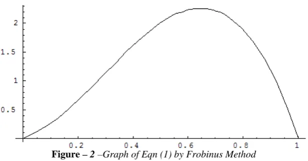
u =1.626954733x -10 x2 +11.17969822 x3 -50.55848491 x4 +47.75233197 x5+.... (5)

The approximated graph of (5) which is the solution of (1) is given below

Figure – 2 –Graph of Eqn (1) by Frobinus Method

Which satisfies the condition of convergence in the interval 0 < x < 1 by virtue of D’alembert’s ratio test. The condition of convergence can be established by introducing the partial sums.

2.3. FINITE DIFFERENCE METHOD

Consider the artificial diffusion – convection equation

2 hx d u

du

ε

₂

x u 1

2 _dx

dx













− +

+

+ =

with

u(0)

=

0, u(1)

=

0

(6)

Apply central difference scheme to the above differential equation where

1 1

u - u

'

u (x)

2 h

i+ i−

=

and

u (x)

u - 2 u

i1 ₂i

u

i 1

h

−

+

′′

=

(7)

Where ui = u(xi). x= ih on substitution of (7) in (6) the new equation is 2

1 1 1 1

2

2 u - 2 u

u

u - u

i h

ε

ih

u 1

2

i i i i i

i

h

− + + −













+

(4)

The final transformed difference scheme is

a u

_i _i₊₁

+

b u

_i _i

+

c u d

_i _i₋₁

=

_i (9) Where

a

_i

=

-

ε,

b

_i

=

2 ε

+

h

2

(

1 i ,

+

)

c

_i

=

-

(

ε i h ,

+

2

)

d

_i

=

h

2

The boundary conditions u(0) = u(1) = 0 are represented by u0 =0, uN =0 Equation (9) represents a Tri-diagonal Matrix of the form

Au

 

=

D

Where the co-efficient matrix A is of order n-1. The Non-homogeneous linear system is solved by applying Thomas algorithm. Here The Co-efficient matrix is a Monotonic matrix. This concept incorporated in this problem reduces the variations in the computed solution. The computed result with corresponding graph is shown below.

.

Figure-3: Numerical solution of the Artificial-diffusion equation.

Table-I: (ε = 0.05)

x u x u x u x u

(5)

3. OBSERVATIONS

It has been observed that the graphs shown in Fig(1), Fig(2), Fig(3) maintain character preserving phenomena over (0,1). Especially in the interval of smooth region steep down fall of the graph coinciding with the actual solution is an appreciable thing of considerable order. For small ε the equation is dominated by the convection term. The boundary or interior layers may appear along downstream of the convection direction i.e., after the smooth region the diffusion effect is visible in the interval (δ, 1). Stable solution is observed under the influence of the artificial-diffusion. The exact solution is non-zero almost everywhere except in a narrow boundary layer sub-intervel very close to the point x=1. The numerically computed values of u also support this statement vide Table-I. The computed solution and the series solution exhibit good agreement on the convection-diffusion phenomena almost through out the the region. Whenever there is very little diffusion then the solution has varrying nature as compared to the exact solution [1]. When diffusion is more (Artificial diffusion), then the computed layers are smeared.

4. REFERENCES

1. D. N.d.G. Allen and R.V Southwell (1955), ‘Relaxation methods applied to determine the motion inn two dimensions, of a viscous fluid past a fixed cylinder’, Quart. J. Mech. Appl. Math. 8, 129-145.

2. V.B. Andreev and N.V. Kopteva (1996), ‘Investigation of difference schemes with an approximation of the first derivative by a central difference relation’, Zh. Vychisl. Mat.i Mat. Fiz. 36(8), 101-117.

3. Arthur E.P. Veldman, Ka-Wing Lam ‘Symmetry-preserving upwind discretization of convection on non-uniform grids., Applied Numerical Mathematics 58 (2008).

4. A. Brandt and I. Yavneh(1991), ‘Inadequacy of firstorder upwind difference schemes for some recirculat -ing flow’, J. Comput. Phys. 93, 128-143.

5. M. Dobrowolski and H.-G. Roos (1997), ‘A priori estimates for the solution of Convection-diffusion problems and interpolation on Shishkin meshes’, Z. Anal. Anwendungen 16, 1001–1012.

6. K.Eriksson, D. Estep, P.Hansbo and C. Johnson (1996), Computational Differential Equations, Cambridge University Press, Cambridge.

7. A. M. Il’in (1969), ‘A difference scheme for a differential equation with a small parameter multiplying the highest derivative’, Mat. Zametki 6, 237–248. equations’, Comput. Methods Appl. Mech. Engrg. 190, 757–781.

8. Introduction to singular Perturbation problems by Robert E.O’s Malley, Jr, Academic press.

9. Martin Stynes (2005) ‘Steady-state convection-diffusion problems‘, Acta Numerica (2005), pp. 445-508, Cambridge University Press.

10. K. W. Morton(1996), Numerical solution of Convection-Diffusion Problems, Vol. 12 of Applied Mathematics and Mathematical Computation, Chapman & Hall, London.

11. Mikhail Shashkov (2005) ‘Conservative finite difference methods on General grids, CRS Press (Tokyo). 12. Dennis G. Roddeman, Some aspects of artificial diffusion in flow analysis, TNO Building and Construction

Research, Netherlands.

13. G.D. Smith, ‘Partial Differential equations’, Oxford Press.

14. N. Srinivasacharyulu, K. Sharath babu (2008), ‘Computational method to solve steady-state convection-diffusion problem’ , International Journal of Mathematics, Computer Sciences and Information Technology, Vol. 1 No. 1-2, January-December 2008, pp.245-254.

15. M. Stynes and L. Tobiska (1998), ‘A finite difference analysis of a streamline diffusion method on a Shishkin meshes’, Numer. Algorithms 18, 337-360.

Source of support: Nil, Conflict of interest: None Declared