Construction Project Scheduling

1

Construction Project

Scheduling

Produced and Distributed by

Engineer Educators

857 East Park Avenue

Tallahassee, FL 32301

2

Disclaimer

The material in this course manual is not meant to infringe on any copyrighted material. The purpose of the course manual is for educational purposes only.

3

Construction Project Scheduling

Table of Contents

I. Introduction to Scheduling and Basic Concepts 2

II. Arrow Diagramming 9

III. Precedence Diagramming 17

IV. Scheduling Computations (Forward and Backward Passes, Floats) 25

V. Project Control 38

VI. Time-Cost Adjustments 43

VII. Resource Leveling 48

4

CHAPTER 1

Introduction to Scheduling and Basic Concepts

History of Construction Scheduling

The most basic scheduling technique was developed during World War I by Henry L. Gantt. It mainly consisted of a bar chart with particular time points indicated on top of it. For many years, this technique was used for expressing project plans. Later on, the construction industry adopted bar chart as an accepted scheduling method not only because it did help visualize the tasks to be done, but also since it facilitated the job of assigning human resources to different activities. However, the very first systematic attempts in utilizing network scheduling with the objective of improving the planning of engineering design and construction started in 1956 when the E. I. du Pont de Nemours Company developed a method upon which the today’s Critical Path Method (CPM) is based. Using a UNIVAC computer, they scheduled a $10 million chemical plant project in Louisville, KY. Soon after, it became apparent that thanks to the fast development of computer interfaces, such network-based systems could easily outperform the traditional manual scheduling techniques. At about the same time, when the U.S. Navy was searching for better techniques for managing large projects such as the POLARIS missile project, the foundation of the Performance Evaluation and Review Technique (PERT) network schedule was established. CPM and PERT were developed independently. However, both methods made use of network graphical models and both identified the critical (i.e. longest) path. Throughout the 1960s, other organizations such as NASA, U.S. Corps of Engineers, RCA, General Electric, the Apollo Program, the Veterans Administration, and the GSA made use of CPM and PERT as well.

Today, with the advancement and widespread use of personal computers, and with more knowledgeable owners, designers, and construction practitioners, network schedules are more widely used. Such scheduling techniques and software designed based upon those (e.g. M.S. Project, Asta Powerproject, and Primavera) not only are commonly used in the planning stage, but also are prevalent during project control and construction.

Significance of Costs and Time

Time is money! The time needed for completion of a construction project and the money required to complete it are most often the major concern to all parties involved in a project. The owner may be interested in shortening each phase of the project or s/he may want to extend the project due to budget cuts, but there is a close relationship between the required cost and time of

5

any construction project. If the project has to be completed in a relatively short time or if its completion takes longer than the expected duration, then the cost will proportionally increase. Construction scheduling ensures construction managers about accomplishing a project in a timely and cost-effective manner. Almost all construction managers admit the role and significance of construction schedules in the successful completion of a project. The type of scheduling technique may vary depending on the characteristics of the project. Sometimes, a very simple bar chart may suffice for a project that may have a relatively high cost and needs advanced work skills, but consists of very few tasks that must be accomplished in a certain prescribed sequence. On the other hand, a more sophisticated case which involves a large number of highly interrelated demanding tasks may require using a more complicated technique such as PERT or CPM. In general, most projects call for more advanced techniques than a simple bar chart, even though the cost of the project is not a considerable dollar value.

What is a Schedule?

Merriam-Webster Dictionary defines the noun “schedule” as “a written document”, “a written or printed list, catalog, or inventory”, or “a procedural plan that indicates the time and sequence of each operation”. It also states that the verb “schedule” refers to “appoint, assign, or designate for a fixed time”. In construction, a schedule refers to a time-based order of activities that are planned to be accomplished in order to successfully (i.e. timely and cost effective) complete the project.

Why Schedule a Construction Project?

Scheduling leads to efficiency! There always should be a plan including what is going to be taking place, the technology involved, the resources needed, and the expected duration for accomplishment of each and every phase of the project, so that the entire project is managed effectively. Such a time-based plan (i.e. the schedule) is very crucial to all the parties involved in a project; an owner wants to know when the project is scheduled to be completed and what is the breakdown to reach important milestones, a contractor must have this schedule to determine the number of and the time during which labor is needed; a vendor requires the schedule for material delivery time; and subcontractors can know if the work can be accomplished in the context of all the other work scheduled.

In activity-level planning, the timing of an activity scheduled start and finish dates can have considerable cost implications. A large crane such as the one shown in Figure 1-1 can rent for as much as $10,000 per week, thus a contractor may end up losing the profit it would hope to get from the job by spending unnecessary money on a rental crane, if the project duration was not

6

properly estimated beforehand. Furthermore, a contractor’s overhead such as site fencing rental, job superintendent salaries, and maintenance of a field office are as well dependent on the duration of the project.

Figure 1.1. A crawler crane can rent for as much as $10,000 per week.

(photo courtesy of Guy M. Tuner Inc.)

When to Schedule?

A document that is usually supplemented to the owner-contractor agreement is “The General Conditions to the Construction Contract” from the American Institute of Architectures (AIA – A201). The “Contractor’s Construction Schedule” Section of AIA – A201 states that:

“3.10.1 The Contractor, promptly after being awarded the Contract, shall prepare and submit for the Owner's and Architect's information a Contractor's construction schedule for the Work. The schedule shall not exceed time limits current under the Contract Documents, shall be revised at appropriate intervals as required by the conditions of the Work and Project, shall be related to the entire Project to the extent required by the Contract Documents, and shall provide for expeditious and practicable execution of the Work”.

Preconstruction

Scheduling during preconstruction is the most common practice. To secure the project financing, owners need to know upfront if the project can be completed on time, so that they can make commitments with the end user. For a retail operation, missing the Christmas shopping season is

7

a great loss. The unfinished 1976 Montreal’s Olympic Stadium affected the planning of the tournament a lot and brought about many unnecessary costs. The one and only way to firmly predict whether or not the required completion dates are reachable is by using a schedule.

During preconstruction, the scheduling should be considered as an opportunity to design and even build the project “on paper” before the actual construction starts. The opportunity is provided for all project parties involved, to visualize the project as a whole and processes in particular, so making required decisions and modifications to collaborate and manage the entire project.

Construction

Not only scheduling is important during the preconstruction phase of a project, but also it is essential during the actual construction period. Material deliveries, modifications to resource allocation and utilization, inevitable delay handling, etc. all happen during the course of the project and require taking necessary actions and updating the schedule accordingly. If it were not for the problems that occur during a construction project, there would be almost no need to have a project manager. So a prompt response to the inevitable delays that result from bad weather conditions, equipment breakdowns, strikes, design errors, etc. and reflecting them in the schedule are all parts of a well-managed project. Figure 1-2 show bad weather that slowed Springbank dam construction in London, and Figure 1-3 shows an equipment failure that resulted in schedule modifications.

Figure 1.2. Bad weather slows dam construction.

Figure 1.3. CAT truck failure.

8

As mentioned earlier, the bar chart is one of the earliest methods for scheduling and controlling construction projects. Although severe limitations may prohibit the widespread use of bar charts when a modern complex structure or infrastructure is targeted and being planned, it has experienced wide acceptance because it can be perceived readily by everyone. A bar chart shows the total project in a compact format and provides the opportunity for visualizing the plan and the progress of the project. A bar chart of a typical building construction project is shown in Figure 1.4. The work has been broken down into 15 major tasks.

Figure 1.4. Bar chart of a typical building construction project.

An Introduction to Network Scheduling

If someone travels from one city to another by car, the assumption is that a highway system can connect that person’s place of residence to his/her objective city. There may be several routes for this travel. Unless the highway map is carefully examined, s/he cannot decide which route is the best in terms of distance, time, road condition, scenic values, points of interest, etc. Such map is considered as a model of the real system and contains a lot of information that eventually lead to a decision.

A construction project can be seen as an objective to be met by a contractor in many ways is similar to the traveler example above. There are many ways to construct a building, for instance, and many routes can be taken to reach the completed product. However, the major difference is that such map is supposed to be created by the contractor and it is not like a highway map, readily available.

9

What is network scheduling?

As a formal definition, a network schedule is a logical and ordered sequence of events that describes in graphical form the approach that will be taken to complete the project. A network consists of two basic elements, nodes, and links between the nodes. In construction management, there are two types of networks. The networks shown in Figures 1.5 and 1.6 both serve as models of building processes and show the same relationships among the activities. It is often the planner’s decision as to which type to choose.

Figure 1.5. Arrow Diagram [2]

Figure 1.6. Precedence diagram [2]

Why network schedules are used?

Networks are used as scheduling tools for effective construction management. A network schedule provides many opportunities for construction managers. It represents a mathematical model for showing the progress of construction activities over time. It also provides a means to do “what-if” analysis, where the user can change one part of the process and observe the effect on the overall project. Network scheduling has also become very important in the settling of legal claims, simplifying the determination of progress payments, analyzing cash-flows, and controlling costs. Many large U.S. government projects require network schedules and many private projects do so as well. Furthermore, the familiarity of the work plan gained while creating the network enhances the ability of the project team to control the actual project.

10

CHAPTER 2

Arrow Diagramming

Characteristics

In depicting the network of activities, the analytical procedure which should be followed requires that the graphics are mathematically expressive. The best way to represent a network and links is to assign an identifying number to the node and denote the link by referring to the numbers at each end.

Unlike a network of pipes and wires in modeling of water or electrical systems, a construction project network also includes information pertinent to unidirectional interactions between nodes. In other words, activities following a node are dependent upon the activities that enter that node, while the reverse is not true. Therefore, there is an analogy between arrow diagraming and piping systems in which a flow is permitted only in one direction and not the other. Putting an arrowhead to the link helps pointing out this unidirectional feature of arrow diagraming.

Ever since network planning began, arrow diagramming has been a popular scheduling technique. One of the most important advantages of this technique is that it has proven to be easily computerized even in case of complex projects with many activities. Moreover, the two-number scheme for identification of an activity provides convenient means for both manual and computerized computations. Also, it can be easily converted to a time-scaled representation which would be similar to a bar chart in which many planners are interested.

One of the features in which many planners have difficulty in using arrow diagrams is dummy activity representation. It nevertheless is important in activity representations since it insures proper interrelationships and therefore will be described in detail in this Chapter.

Logic Patterns for Arrow Diagrams

Arrows in representation of activities should not be confused with vectors, as the length, shape, and orientation of the arrow has no significance. In order to suit the needs of the graphical representation, the arrow could be straight, curved, bent, or wavy. The purpose of the diagram is to establish the logic of the project and identification of the order of the tasks. A few types of logic statements and their diagrams are shown in Figure 2.1.

11

Figure 2.1. Some logic statements and corresponding diagrams. [3]

Each activity has a definite beginning and end represented by the nodes at each extremity of the arrow. The nodes are commonly called “events” as they mark points in time and have no durations. Usually, the event at the tail of the arrow is called the “i event” and the one at the head is called the “j event” as shown in Figure 2.2.

Figure 2.2. Basic activity. [2]

Two activities are called independent, when there is no direct arrow connecting them to each other. Figure 2.3 shows an example of this condition.

12

Figure 2.3. Independent activities. [2]

When an activity is dependent upon another, they appear as two arrows with a common node in the diagram. Figure 2.4 illustrates this logic, in which node 6 serves as the i node of Activity B and at the same time the j node of Activity A.

Figure 2.4. Dependent activities. [2]

Often times, there is an activity that cannot be started before completion of two or more activities. This is called a “merge” condition and is shown in Figure 2.5. On the other hand, there frequently is another condition in which two or more activities cannot be started until a third activity is completed. In this case the diagram contains a “burst” condition which is shown in Figure 2.6.

13

Figure 2.6. Representation of a “burst”. [2]

In a combined condition, when two or more activities must be finished before two or more activities can start, the resulting diagram is said to contain a “cross” as illustrated in Figure 2.7. Note that in this case, neither Activity C nor Activity D can start until both Activity A and Activity B have finished.

Figure 2.7. Representation of a “cross”. [2]

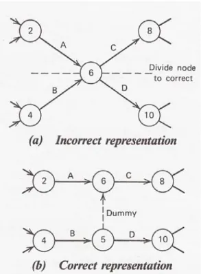
Dummy Activity

When one activity is dependent upon the preceding activities and another is dependent upon only one of the preceding activities, then the accurate representation of this situation cannot be shown by a cross. For example, imagine activity C depends upon the completion of Activities A and B, but Activity D depends only upon completion of Activity B. The cross diagram which is shown in Figure 2.8.a is an incorrect representation of this situation. To correct this logical error, Event 6 can be divided into two events numbered 5 and 6, and another activity can be inserted between them. This activity is called a “dummy activity”, which is a fictitious activity that not only does not have any duration, but also requires no resource utilization. The correct representation is shown in Figure 2.8.b.

14

Figure 2.8. The use of the dummy activity to define correct logic in an arrow diagram (Activity C depends upon Activity A and B. Activity D depends upon Activity B only). [2]

Another use of a dummy activity is in situations where there are two or more activities that depend upon the same preceding activities and have the same following activities also. In order to avoid confusion when each activity is described by its event numbers, the numbers should be unique for each activity. Figure 2.9.a shows activities A and B that begin and end on events 10 and 12 that are in common. Therefore, if one is to describe both Activities A and B by the numbers 10-12, this leads to confusion. In order to avoid such confusion the tail node should be divided and a new event with a dummy activity connecting the new and original event should be created. The correction made has been illustrated in Figure 2.9.b.

15

Figure 2.9. The use of the dummy activity to maintain unique numbering of activities. [2]

Numbering the Network

Numbering the events at each end of the links (i.e. activities) is not done until the diagram is finished. Generally, numbers “i" and “j” are assigned arbitrarily. However, usually they are numbered in such a way that the number at the head is bigger than the one at the tail. Care must be exercised to make sure that each event in the network has a unique number. Consecutive numbering might seem to be a good idea since it guarantees directionality and uniqueness, although it does not allow the addition of future activities.

Constructing an Arrow Diagram

The process of drawing the arrow diagram has no easy direct approach. The need for dummy activities introduces situations that are too variable to defy a systematic approach. However, constructing a diagram is described here through an example.

16

The retaining wall shown in Figure 2.10 is to be constructed.

Figure 2.10. The retaining wall for which an arrow diagram is to be drawn. [2]

It is assumed that both the wall and the footing have a construction joint at mid-length resulting in four parts to be built as shown in the Figure 2.10. In addition, assume that it is desired to start with the first half of the footing. The initial event is shown in Figure 2.11 with activity Footing 1 following it. The second event and two succeeding activities, Footing 2 and Wall 1, are also given.

Figure 2.11. First part of the arrow diagram. [2]

Wall 2 is added in Figure 2.12.

17

Now it is the time to check for possible needs to dummy activities. Adding Wall 1 calls for a dummy activity in order to preserve the numbering uniqueness for the activities. Figure 2.13 shows the final diagram with this correction and events properly numbered.

18

CHAPTER 3

Precedence Diagramming

Introduction

Although CPM was initially built upon the concept of arrow diagramming, Professor John W. Fondahl (Stanford University) in 1961 introduced a new CPM representation based upon precedence diagrams. The transformation rule was simple: as opposed to assigning activities to links, Fondahl placed them on nodes. Therefore, the links that connect nodes (i.e. activities) represent the relationships between them. This type of diagramming was initially called “circle and connecting line”, but that name was replaced with “precedence diagram” or “activity on the node”.

A precedence diagram is proven to have several advantages over arrow diagrams. First and foremost, there is no need to use dummy activities to define network logic. Second, as opposed to having two-number representation for each activity, only one number suffices in this type. Third, the analytical procedure to be carried out on computers is easy and much more straightforward.

Logic Patterns for Precedence Diagrams

Similar to arrow diagrams, in the precedence diagrams the focus is again on activities. An activity in a precedence diagram is represented by a number enclosed in some kind of symbol (e.g. circle, square, hexagonal). As mentioned earlier, the relationships between the activities (i.e. nodes) are expressed by links drawn from one activity to the other. When two activities are independent of each other, there will be no linkage between the two on the diagram, as shown on Figure 3.1.

19

If the two activities are related so that starting one of them is dependent on the completion of the other, then the nodes are linked. Figure 3.2 shows an example in which Activity A should be completed before Activity B can be started.

Figure 3.2. Dependent relationships. [2]

When two or more activities must be completed before a common activity can start, a “merge” relationship will appear in the diagram. Such case is shown in Figure 3.3 in which both Activity A and Activity B should be finished in order for the Activity C to be started.

Figure 3.3. Merging relationships. [2]

Likewise, in case two or more activities depend upon the completion of a common activity, a “burst” relationship will appear in the diagram. Figure 3.4 pictures this situation for the linkage between Activity B and Activities C and E.

20

Note that if an activity is known to be related to two activities which at the same time are related to each other, a redundancy would be created in the diagram that should be removed. Figure 3.5.a depicts an example of such situation.

Figure 3.5 Redundant linkage[2]

In this Figure, Activity C in known to be related to both Activities A and B and at the same time Activity B depends upon Activity A. The link that connects Activities A and C is redundant in order to satisfy the logic of these relationships. Because if Activity C depends upon the completion of Activity B, and Activity B depends upon the completion of Activity A, then Activity A have to be completed before Activity C can start. To detect such redundancy one should look for the “triangle pattern” that is formed in the diagram. Figure 3.5.b shows the correct relationship.

It frequently happens that several activities can be considered as the starting activities of a project. Likewise, very often, more than one activity marks the completion of the entire project. Therefore, the final diagram would contain several nodes without links to preceding activities and several others without links to succeeding activities. Since some computer programs require the network to start and finish with a single activity, a dummy activity or “event node” can be introduced to start and finish the network. As an example, a network of five activities is shown in Figure 3.6.a.

21

Figure 3.6. Closing the network to give single beginning and ending nodes. [2]

As shown in this Figure, Activities A, B, and C are independent of each other, whereas Activity E depends upon the completion of activity A and Activity F depends upon the completion of Activity C. Although the logic among this configuration of the network is correct, there are still open beginning nodes (A, B, C) and open ending nodes (E, B, F). The logic for the start and finish is not correct. The correct representation is shown in Figure 3.6.b in which two dummy activities have been added to the start and finish of the network.

To summarize all the logic patterns discussed above, consider the retaining wall example from Chapter 2. Here is the problem statement again: a retaining wall consists of a spread footing and a vertical stem for which a precedence network is to be drawn. The wall and the footing each have a construction joint at mid-length so that there are four portions to consider. The assumption is that the start of the construction is with the first part of the footing and that the second part of the wall is to be cast against the first part of the wall. Figure 3.7 depicts the precedence diagram for this project.

22

Figure 3.7. Retaining wall precedence diagram. [2]

It should be noted that Activity 20 (Footing 2) and Activity 30 (Wall 1) are independent meaning that either could be cast after Footing 1 is completed but they are not dependent upon each other. A burst relationship can be seen that is formed Activity 10 and Activities 20 and 30, and a merge relationship is set up by the two links between Activities 20 and 30 and Activity 40. It is clear that in this example, it is not necessary to use dummy activities at the start and finish because the diagram itself closes with single nodes.

Numbering and Drawing the Network

In order to obtain a clear understanding of the logic of the network, there needs to be an ordering scheme. Also, the computation to be made using the precedence diagram requires that numbering pattern be set up to maintain the network directionality. These objectives are met by placing the activities in a “sequence step” order. A sequence step is the earliest logical position in the network that an activity can occupy while maintaining its proper dependencies. This definition can be fully understood by referring to Figure 3.8.

23

Figure 3.8. Precedence diagram – sequence stepped and numbered. [2]

The activity Start as the beginning activity has been placed on Sequence Step 1. Activities A, B, and C, each of which are dependent upon Activity Start, have been placed one step to the right and appear on Sequence Step 2. Activities E and F are placed on the step following their dependencies on Step 3. Finally, Activity Finish is on the Step 4, one step from its dependent Activities E and F, and two steps from Activity B. Note that in order to comply with the abovementioned rules and definitions, Activity B is at the earlier of its two possible logic steps. To each activity in the network, one unique identifying number should be assigned. The numbers assigned arbitrarily during the creation of the activity list can be used by some computer programs but this is not an efficient practice. It is better to give numbers to activities after the completion of the diagram and the arrangement of sequencing step orders. To satisfy the directional requirements of the network, it is recommended to assign the activity that appears at the left end of a link a smaller number than the one assigned to the right end.

Although consecutive numbering may satisfy the requirements of directionality and uniqueness, it does not permit the addition of future activities without changing the numbering pattern of the whole network. Instead, a better numbering scheme may be achieved using even or odd numbers, numbers by fives or tens, or some similar patterns. It is very likely that during the creation of a network diagram (often, the planning stage) not all project activities are known. Therefore, the numbering pattern that is selected should reflect the quantity of anticipated additions. In the precedence notation, one is able to overlap activities by using a characteristic called “leads and lags”. The use of leads and lags which is illustrated in Figure 3.9 is a recognition of the fact that project operations are not perfectly sequential and that often activities run in parallel, or are phased with certain activities being given a head start.

24

Figure 3.9. Arrow notation compared to precedence notation. [3]

Arrow diagrams can handle these complexities with certain additional activities as illustrated in Figure 3.9. The same operational sequence could be shown in precedence notation by the use of Start to Start, Finish to Finish, and Start to Finish relationships. As shown in the bottom of

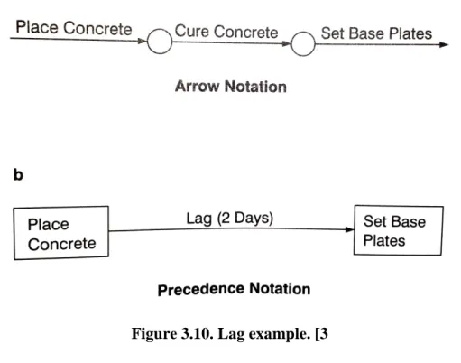
25

Figure 3.9, the starting of an activity can also be delayed by the use of what is called a link duration or lag. A good example might be in sequencing the placement of concrete followed by the setting of base plates. The specifications call for a 2-day curing of the concrete before the base plates can be set. Figure 3.10 illustrates both arrow and precedence notations of this lag example.

Figure 3.10. Lag example. [3

As shown in Figure 3.10, precedence notation needs fewer activities and can model the job sequence faster. That is perhaps why many companies and software packages are now set up to comply with and utilize the precedence notation.

26

CHAPTER 4

Scheduling Computations

Introduction

Scheduling is about timing. Assigning proper durations to activities can lead to a successful project scheduling. Sometimes, it is straightforward to establish these durations, but most of the times it is not so easy to formulate durations. The most basic measure to choose for establishing durations is the time interval. Next, an estimate of the time duration for each activity must be made. These durations may be established from the company’s historical field data or may be obtained from direct interviews with the field personnel.

Time Intervals for Network Scheduling

Seconds, minutes, hours, days, weeks, months, years, and decade, are all acceptable time intervals to be used in construction scheduling. Choosing the right one might be obvious or may need to be derived from customary practice. The amount of time required to perform an activity determines the time interval that is better to be selected for scheduling. For instance, it is not appropriate to use days as the base if most activities require only a few hours to be completed, or to use hours for an activity that its completion takes several days.

The usual practice in commercial construction is to use calendar days as the basic interval of the project. Most frequently, the customary employment period of the activity resource is adopted as the basic time interval for scheduling. Within construction industry, labor is usually paid an hourly wage but employment period is commonly the 8-hour working day, and therefore, the working day is the basic scheduling interval in construction. Similarly, the 5-day, 40-hour work week is often used as the base for large projects.

Regardless of the time interval selected, the consistency of using that throughout the network diagram is of more importance. If the working day is being used as the basic interval and there are several procurement activities with durations expressed in calendar days, the procurement durations have to be adjusted to reflect the basic interval selected. For example, an item that has a 30-day delivery will actually consume only 22 working days if a 5-day week is being followed and 26 days if a 6-day week pattern is used.

27

Estimating Activity Durations

Choosing the right duration for each activity is very critical and needs accurate analysis. Off-hand estimates of activity time have not been proven to be satisfactory. Sometimes, the planner chooses the initial time casually offered by the company estimator as the most probable duration for an activity, but unless the estimator has recorded durations from past projects, the estimate might be off the true value by as much as 100% or more!

There are typical estimate guides that give the costs to perform work in terms of dollars per unit of material, such as “$50 per cubic yard” or “$20 per square foot”. Such estimates are based on the tacit assumptions of a commonly used method and a customary utilization of human resources and equipment. In most construction firms, sometimes records are not available in a manner that let the planner determine the time it takes to do a particular task. Because activity durations are to be used in CPM technique, certain steps must be taken by the planner to derive the duration from sources other than the estimating department or the company’s history.

Scheduling Calculations

Assume that in this step the project management team knows the logic of the project, all

activities that are supposed to be included in the schedule, and the duration of each activity. Now it is time for scheduling calculations. Scheduling computations will eventually determine the length of the project, start and finish time of each activity, and the activities than can be slipped for some specific amounts of time without affecting the completion date of the project. In

scheduling calculation, each activity in the network has four values associated with it on the time scale, as follows:

Early Start (ES): The early start of an activity is the earliest possible time that an activity can start based on the logic and durations identified on the network.

Early Finish (EF): The early finish of an activity is the earliest possible time that an activity can finish based on the logic and durations identified on the network. Basically, early finish of an activity is equal to the early start plus the activity duration:

Early Finish = Early Start + Duration

Late Finish (LF): The late finish of an activity is the latest possible time an activity can finish based on the logic and durations identified on the network without extending the completion date of the project.

Late Start (LS): The late start of an activity is the latest possible time that an activity can start based on the logic and durations identified on the network without extending the completion data

28

of the project. Basically, the late start of an activity is equal to the late finish minus the activity duration.

Late Start = Late Finish – Duration

Float: The float of an activity is an additional time that an activity can use beyond the duration that has been originally defined for it yet not to cause a delay in the completion date of the entire project. Mathematically, float can be defined as late finish minus early finish or late start minus early start:

Float = Late Finish – Early Finish = Late Start – Early Start

Forward and Backward Pass Calculations

In case of using activity on arrow notation, two forms are commonly used to calculate the “node times” or “event times” for the network. A node time indicates the amount of project time that must be consumed to get to that node in the schedule. As illustrated in Figure 4.1, the early time identifies the earliest possible time that the project can get to a certain node in the network if the logic and durations are followed. Forward pass calculation is used to compute this time which is the early start time for all activities which originate at that node. The late time shown in Figure 4.1 indicates the latest possible time that the project can be at this point in the network without extending the completion date of the project. Backward pass calculation is used to compute this time which is the late finish time for all activities which terminate at this node.

29

Figure 4.1. Node times on arrow diagram. [3]

In case of using precedent notation, activity node contains all activity times and float as shown in Figure 4.2. In this notation, the forward and backward pass calculations are done internal to the activity, with the node times equal to the activity times.

30

In either case (i.e. arrow or precedence diagram), forward pass is the first calculation to be made. The calculation starts with the first node assigned “time 0” and the duration of each successive activity added to this time. When using arrow diagram, the i node time of an activity with only one precedent is equal to the i node time of its precedent plus it precedent’s duration. In precedent notation, the early start time of the activity with only one precedent equals the early finish time of the preceding activity. This is shown in Figure 4.3.a and 4.3.b for arrow diagram and precedence diagram, respectively.

Figure 4.3. Forward pass with only one predecessor for (a) arrow diagram, and (b) precedence diagram. [3]

However, when there is more than one predecessor for a node, the early node time in activity on arrow notation equals to the largest time calculated from the converging paths. In the precedent notation, the early start time equals to the largest early finish time of the preceding activities. This is shown in Figure 4.4 for both arrow and precedence diagrams.

31

Figure 4.4. Forward pass with multiple predecessors. [3]

Figure 4.5 illustrates a forward pass for a simple network diagram in both arrow and precedence notations. Note (in the precedence diagram) the use of both finish to start and start to start links and the placement of durations on the links. For example, an SS2 means that the following activity can start 2 days after the preceding activity starts. An FS2 means that the succeeding activity can start 2 days after the preceding activity finishes.

32

Figure 4.5. Forward pass calculation example. [3]

Following the completion of the forward pass, the backward pass can be conducted. The backward pass cannot be done until the project duration is known. The backward pass calculations begin with the last node in arrow diagram notation, or the last activity in the precedence notation. In the former, the project duration is the late event time for the last node, and in the latter, the project duration is the finish time for the last activity. The reason why it is

33

called backward pass is that it is completed by working backwards (from finish to start) by subtracting the activity’s duration from the previous late time. In the arrow notation, the late event time at the j node of an activity with only one successor is equal to the late event time at the j node of the successor minus the successor’s duration. In the precedence notation, the late finish time of an activity with only one successor is equal to the late start time of the successor. This is shown in Figure 4.6.a and 4.6.b for arrow diagram and precedence diagram, respectively.

Figure 4.6. Backward pass with only one predecessor for (a) arrow diagram, and (b) precedence diagram. [3]

When a node has multiple successor activities, the node’s late event time is equal to the smallest of the succeeding nodes’ late times less the activities’ durations. In the precedence notation, the late finish time of an activity equals to the smallest late start times of all the succeeding activities. This is shown in Figure 4.7 for both arrow and precedence diagrams.

34

Figure 4.7. Backward pass with multiple successors. [3]

Figure 4.8 shows the complete example that was previously displayed in Figure 4.5, this time using the backward pass calculation. Pay attention to the use of dummies and lags.

35

Figure 4.8. Backward pass calculation example. [3]

Float Calculations

Activities can be done either early or late. As defined earlier, the difference between the late start time and early start time is equal to the difference between the late finish time and the early

36

finish time which is called float. In order to fully understand the concept of the float, Figure 4.9 is examined.

Figure 4.9. Example project for float calculations. [3]

As can be seen in the arrow diagram of Figure 4.9, there are nine paths through the network, each having its own duration (as an exercise, try to find these paths and durations for the precedence diagram):

37

1. S-5-10-20-30-40-55-65-F Duration = 15

2. S-20-30-40-55-65-F Duration = 13

3. S-20-30-35-45-55-65-F Duration = 15

4. S-20-30-35-45-50-60-65-F Duration = 17

5. S-5-10-20-30-35-45-55-65-F Duration = 17

6. S-5-10-20-30-35-45-50-60-65-F Duration = 19

7. S-5-10-15-35-45-55-65-F Duration = 16

8. S-5-10-15-35-45-50-60-65-F Duration = 18

9. S-5-10-15-25-50-60-65-F Duration = 17

For example, consider the longest path (path 6) that has no float. This means that any delay that occurs in any of the activities in this path will delay the completion of the entire project. Also, notice that the float for each activity in this path equals to 0. This is called the critical path

because any delay in activities in this path will delay the entire project.

Consider path 2 with 13 days duration in which two activities have 0 float and two activities have 4 days of float. It is not possible for both activities 30-40 and 40-55 to use their 4-day float, because if 30-40 uses the 4 days of float, then 40-55 becomes critical. The float that was defined above is called total float, which is the amount of time an activity can be delayed without delaying the overall project duration. Another type of float is free float which is measured by subtracting the early finish (EF) of the activity from the early start (ES) of the successor activity. Free float represents the amount of time that a scheduled activity can be delayed without delaying the early start date of any immediate successor activity within the network path. In case of activities 30-40 and 40-55 in Figure 4.9, 30-40 has 0 days of free float since if it uses any float it will be delaying the early start of activity 40-55. However, 40-55 has 2 days of free float because it can be delayed by 2 days without impacting its immediate successor.

Critical Path

Critical path is the sequence of activities which add up to the longest overall duration. It is the shortest time possible to complete the project. Any delay of an activity on the critical path directly impacts the planned project completion date (there is no float on the critical path). Note that there can be more than one critical path in a project. It is important that the project manager identify these paths and carefully evaluate them, because controlling the time on these paths defines the control of the project. Figure 4.10 shows critical paths on both arrow and precedence diagrams.

38

39

CHAPTER 5

Project Control

Introduction

The dynamic nature of construction projects requires constant monitoring of all project operations. The actual work, cost, and duration must be continuously documented and frequently compared to the original work. Any deviation should be carefully examined and adjustments should be carried out accordingly.

Forecasting is as well an important part of the project control process. The expected cost and time for project completion must be continually updated and reported. The control process must document progress and allow project team to adjust to conditions that were not anticipated, such as equipment breakdown, unstable weather conditions, and change orders. A control process includes a reporting system to notify all necessary parties of the project status. This lets outside experts and senior management teams to make adjustments to the original plan as necessary. Finally, the project control system is an iterative process, meaning that the process occurs over and over, encouraging a continual adjustment to the plan of the project team.

Project Control Objectives

A good and effective control plan seeks to accomplish three major objectives. First and foremost, the plan should accurately represent the work and allow it to be carried out to some extent compatible with the designed plans and construction specifications. Second, the plan should allow for deviations from the schedule to be detected, evaluated, and forecasted. And finally, the plan should make provision for periodic corrective actions to economically bring any remaining schedule into alignment with the proposed schedule.

A project control system begins with the establishment of project standards. Project management team uses such standards to continuously check the progress against acceptable standards. Standards for a quality control would be defined by the drawings and specifications. Drawings define the quantity of work required, locations, and widths and heights. Specifications, on the other hand, define the quality of the work, defining performance standards, addressing issues such as alignment, compression strengths, and finishes. The overall budget for the project as well as milestone costs for specific phases of the work is established by the project estimate. The schedule defines the time when each specific work item needs to be accomplished. Estimate data

40

can be integrated with schedule information to provide additional project standards for the project.

Levels of Control

There are many variations for project control plans. The specific scheme to be used is chosen based on factors such as the size and structure of the construction firm, previous experience of the organization, the urgency of project duration satisfaction, the demands of the owner or regulatory agency, and the size of the project. The project size is the most important one of these factors for the contractor. Large projects usually require greater control than small ones.

For small, low-cost projects with a short duration, the minimum control plan needed is a detailed network and some kind of reporting mechanism, a two-level scheme. In such projects, the duration is considered as a milestone date and the contractor develops the network and schedule to meet this milestone. The scheme is used to prepare a day-by-day budget for the costs to be incurred during construction.

In large projects that have many milestones, take a long time to complete, and cost great sums of money, the levels of control are more complex. In most cases, the contract is negotiated and may be of the cost plus a fee type. Drawing milestone network developed during the earliest stages of the project development is the first level of control. This network is used in conjunction with the schedule by the construction manager when reporting the project schedule to the owner.

The next level of control for both small and large projects is preparing a summary network to advise the upper levels of the management team. This diagram is prepared by the project planning engineer with input from all responsible parties. A third level almost always consists of area and craft networks and schedules. A fourth level consists of detailed networks and schedules prepared for engineering personnel and craft supervision.

Target Schedule

A target schedule is the time schedule that is going to be used for the schedule. While the network calculations result in start and finish limits for each activity, it is usually recommended to provide field personnel with a schedule where each activity has only one start time and one finish time, which constitute the target schedule. The target schedule is somewhere between the early start and late start schedules. A good way to look at this is through using “S-curves” which plot resource expenditure versus time. Figure 5.1 shows S-curves for a typical project. Noncritical activities have varying amounts of float available so make starting between the early start and late start possible. In case of critical activities, however, the early start and late start dates are the same.

41

Figure 5.1. Target schedule S-curve. [2]

Project Monitoring

Construction managers must continuously monitor the work progress to determine whether the project is meeting the planned schedule. Monitoring requires that provisions be made to get feedback from various field resources about the progress of the project. In small projects this may be a relatively simple task, whereas in more complex ones, more sophisticated sets of internal reports, checkoff lists and charts may be needed to get required feedback.

Feedback can be obtained from direct contact and field observations, and requires a close cooperation between the manager and filed personnel. Feedback may also be received from photographic means. For many years, photography has been used by contractors to keep records of progress and to provide permanent documentation of the work which could be helpful in providing feedback to construction manager. Also, many construction managers adopt checkoff techniques to increase the accuracy of the feedback. A checkoff is a list of activities (prepared by the planner) that are to be started, to continue, or to be finished during the next time interval. The superintendent should check the appropriate column to indicate the accomplishment of the work. Feedback can be also obtained from bar charts in which additional information is added during the course of the project. A sample of such bar chart is shown in Figure 5.2.

42

Figure 5.2. Project control bar chart. [1]

Updating the Schedule

Another phase of a good project control is updating the schedule. This process involves the correction of the target plan to economically meet the project’s overall objectives, which are completion within the planned time and budget. It consists of planning and scheduling the remaining work after the project made some progress. Updating is a very important step in successful CPM use and is a vital part of the project control. In updating, the scheduler notes what has happened prior to the time of update and modifies the schedule accordingly. The new (updated) schedule that is generated as a result, shows the schedule for the future, and in combination with prior versions of the schedule, can show when delays, accelerations, and changes took place. This information is needed for project control, cost accounting, claim resolution, etc.

It is important to remember that a CPM schedule is only a plan for a real phenomenon and is not a mandatory sequence of actions. That is why everything in the original schedule is subject to change. There are three possible changes:

1- Change in the duration of an activity.

2- Addition or removal of an activity.

3- Change in the logical relationship between activities.

To update the schedule, all actual data to date in addition to the latest time estimates for future activities are needed. As the project makes progress, it is desired to see how the progress is with regard to the target schedule. This is done by monitoring the progress and using the feedback that was obtained to update the schedule. The physical recording of actual progress can be done by marking up the target schedule and/or by keeping the records in tables. One important practice in monitoring is exception report; that is, once the target schedule is set, any activities

43

accomplished as planned are not reported, but any activities that are off the plan considering an acceptable tolerance should be reported.

Update should be done when it does not bring about further costs. An optimum somewhere should be sought between continuous updating and no updating. The proper frequency depends on many factors, so the frequency should be set in a way that is the most time effective. The most common updating frequencies are those based on contract requirements, fixed time intervals, and milestone based. Many contracts require a schedule update as part of the contractor monthly payment request. When there is not such a mandate, a fixed time is considered that can be monthly or otherwise. Also, the significant events or milestones provide natural points at which it is good to do the updating and review the progress.

44

CHAPTER 6

Time Cost Relationships and Adjustments

Introduction

Project duration has great impact on the overall cost of the project. For any given project, the duration may be estimated by the contractor using previous experiences with similar work or based on the dollar volume per unit of time to which his/her firm is accustomed. On the other hand, the owner may be willing to specify duration for the project in a way that suits his/her requirements. Duration can also be determined by the demands of the weather.

Regardless of the approach taken to estimate the project duration, it is only after a contractor has signed a contract that the network is detailed and exact project duration is revealed. This duration may turn out to be greater than what is promised in the contract and therefore, adjustments must be applied to reduce the project duration to fall within the contractual time limit.

Activity Time-Resource Concepts

As stated before, activity duration depends on (1) the construction method to be used, as well as (2) the quantity of the work involved. Once the construction method has been selected, the resources for that activity can be established. Two concepts should be noted in selecting and allocating the resources. The first is that there is a relationship between the rate at which a resource is applied to an activity, and the cost rate. The second is that there also is a relationship between the total amount of resource applied and the duration for an activity.

There is not a basic straight line relationship between the resource rate (resource units divided by the time interval) and cost rate (dollars per time interval). Because it is commonly assumed that if there is a possibility to assign more than one unit of resource to an activity, the one that has the least cost will be assigned first. Therefore, the cost per unit of time for doing an activity will increase more rapidly as the resource rate increases. This is shown qualitatively in Figure 6.1 by curve A. Such increases are mainly due to activity overhead costs.

45

Figure 6.1. Resource rate-cost relationships for an activity. [2]

In this Figure, curve B illustrates the variation that might take place if the assignment of resources is made by the most costly unit first. This is not a usual pattern, but there are exceptions in such format. The resource rate is the crew size when the resource is that of manpower and the increase in cost may come about because of the increasing cost of supervision, for instance. When the rate is a measure of the equipment, the increase stems from the greater ownership and operating costs required by the added units. In the case of material as the resource, the increase is the result of handling cots for a larger amount of material.

Activity Time-Cost Relationships

Most of the activities in a network have some kind of time-cost relationship and the variations in the time and cost is usually linear. Figure 6.2 illustrates a generalized activity time-cost relationship.

46

Figure 6.2. Activity time-cost relationships. [2]

In this Figure, the point labeled N is the minimum cost point. The coordinates of N are CN and TN on the cost and time axes, respectively. Point C is the minimum time point and is indicated by coordinates TC and CC on the time and cost axes, respectively. The dashed curve suggests the true curve between points C and N. Point N, representing the minimum cost is called the normal point and is the commonly sought as a condition that every contractor would hope to achieve. Point C, the minimum time point, is called the crash point because its achievement implies expending a lot of effort to reduce the time to this minimum. There is another point in Figure 6.2, E, shown on the line between C and N. This represents the conventionally derived estimate of the activity duration and cost.

Project Time-Cost Relationships

The overall construction project cost is divided into two types: indirect costs and direct costs. Indirect costs generally refer to those that apply to the project as a whole. Direct costs are those that can be assigned to the individual activities.

47

Indirect Cost

The indirect cost is the money spent on doing business, which is the general overhead that a construction firm must carry. The cost of secretarial assistance, telephone services, heat and light of the central office, managerial expenses of cost accounting, payroll, bid preparation, and scheduling all fall in this category.

The second main group of indirect costs refers to those that apply to particular contracts, such as operating the site office, applying special safety programs, supervising the job, etc. Also, when a contract has a “liquidated damages” clause and/or a “bonus” clause is included, any related charges are considered as indirect costs. A typical indirect cost curve is shown in Figure 6.3.

48

Direct Cost

Costs directly assignable to each network activity can be added together to obtain the direct project cost. Individual activities can be performed at any duration between the normal and crash points. Therefore, there is a wide range of possible combinations of schedule times and costs for every possible project duration. The combination of activity times and costs that results in the minimum value at every project duration results in the minimum direct project cost curve. A typical minimum direct cost curve is shown in Figure 6.3. Unlike the minimum direct cost shown on this Figure, if conventional estimating procedures determine the costs and duration of activities, the subsequent project time and cost may not fall on the minimum curve. Instead, it will lie somewhere above the curve labeled as CE in this Figure.

Total Cost

The sum of the indirect and direct costs at any time results in the total project cost at that specific time. Plotting these values for all possible project duration times gives the project total cost curve. This total cost curve is illustrated as the upper curve in Figure 6.3. The minimum total cost occurs at the duration where the slopes of the indirect and direct cost curves are equal. If equality cannot be obtained, the minimum point will occur where the slope of the total cost curve changes from negative to positive. This point is labeled as TM in Figure 6.3.

Schedule Compression

The systematic process of arriving at the least-cost solution is sometimes called schedule compression. Least-cost scheduling is an optimization process whereby project activities are shortened in order to shorten the overall project lengths. When activities are shortened, their direct costs increase, but with reducing the overall project duration, indirect costs decrease. So the optimized solution is the one in which the indirect cost savings are greater than the increased direct costs.

49

CHAPTER 7

Resource Leveling

Introduction

Activities can start in their early start dates, or in other words, as soon as it is logically (based on the established precedence logic) possible. However, activities other than those on the critical path may have some float that can let them to be scheduled to start at later dates. By choosing to schedule such noncritical activities at other than their earliest possible times, the demand for the resources on various project dates can be altered (i.e. reduced). The process of making these adjustments is called resource leveling.

Through resource leveling, resources are assigned in a manner that will improve productivity and efficiency. Leveling procedures for construction work can be effective in the management of all kinds of resources. The most common resource to be considered for leveling is labor, as he need for leveling workforce stems from the desire to maintain the lowest possible number of employees to perform the work.

All types of projects have potential of being leveled and that is independent of the type of the network that is used for scheduling, although the network influences the results in many leveling procedures.

Two heuristic approaches are used for resource leveling. The objective of the first approach is to minimize the levels, and thereby the costs. The objective of the second one is to minimize the duration (total time) of the project. The first set is called “Unlimited Resource Leveling”, and the second set is called “Limited Resource Allocation”. The latter is referred to as the traditional method in this Chapter. Another method which is called the “Minimum Moment Algorithm” addresses the leveling problem by considering the resource histogram as an area in the time-resource field and sets its objective as to minimize the moment of that area.

Objectives

There are a number of reasons why a planner may feel the need to use resource leveling, including the following three major needs:

1- The need to meet the physical limits of the resources.

2- The need to avoid the day-to-day fluctuations in resource demands.

3- The need to maintain an even flow of application for the resources.

50

The traditional approach in resource leveling starts with adding up (for each day) the resource rates for each activity scheduled in its early start schedule position. These sums are called the daily resource sums.

An evaluation of activity resource rates indicates a possible minimum level that can be assumed as an upper limit on the daily resource sums. Next, starting from day 1, the resource demands are evaluated day-by-day to see if they are less than or greater than the assumed value. If the demand exceeds the assumed limit an activity is selected from a priority list and shifted one day. Again the daily resource sum is examined and another activity shifted until the demand has been reduced below a limit. As soon as the day’s limit is fixed, the next successive day is examined using the same procedure. This iterative process continues until the project duration is reached. If there are still demands greater than the assumed limit, the project is extended in time, until all the daily resources sums are below the assumed limit.

Figure 7.1 is an example to better describe the process. The arrow diagram in this Figure corresponds to a sample project consisting of six activities. Figure 7.2 shows the precedence diagram for the same project. Table 7.1 contains necessary information about the six activities as determined from the early start calculations. The product of the resource rate and the activity duration appears in the last column of the Table. The total of 49 (as shown at the bottom of this Table) indicates the total resource load for the project.

51

Figure 7.2. Precedence diagram for the resource leveling example. [2]

Table 7.1. Resource leveling calculations. [2]

The upper section of Figure 7.3 contains a bar chart of the project. The name of each activity together with the resource rate of that activity is written on top of each bar. Note that the critical activities are plotted first, so that noncritical activities with float can be recognizable quickly.

52

Figure 7.3. Resource leveling example. [2]

In this Figure, the sums of the resource rates for each day are included right below the bar chart. The daily resource sums appear in the row marked by ∑0. For an ide al uniform level, the sums would average 4.9 units because the project duration is 10 days. This Figure could have been used as the assumed resource limit. However, there is one activity in the network that has a daily resource rate of 6 units. Therefore, the minimum level that can be assumed to still complete the project within the specified duration is 6 units.

Figure 7.3 shows that the first day has a resource demand of 4 units. This is less than the assumed 6 days and meets the test. The second, third, and fourth days are also satisfactory. The fifth day has a demand of 10 resource units and therefore, some activities must be shifted to reduce this value to less than or equal to the assumption (6 units). Activities C and D are both scheduled to start on the fifth day, but D is critical and cannot be shifted. Thus, Activity C is selected and shifted one day and rescheduled on days 6 and 7.

The shifting of activity C is illustrated by the subtraction of the resource rate of 4 units from the sum for day 5 and adding this same rate to the sum for day 7. The revised daily resource sums for days 5, 6, and 7 are shown on the row marked by ∑1. The fifth day is now within the assumed 6 unit limit.

53

The sixth day is evaluated next and the same reasoning leads to an adjusted daily resource sum for that day. The process continues for days 7 and 8. On day 9, there are two noncritical activities to be examined. Activity C had used all its available float and therefore, the only activity that can be moved is Activity E. The revised sums are shown on the row marked by ∑5.

On day 10, both Activities C and E have used all their floats and are now considered critical. Therefore, the only remaining option for reducing the daily resource sum below the assumed limit of 6 is to lengthen the project duration. The extension is done while keeping in mind that the choice for shifting must decrease the daily sum below the limit and at the same time, must result in a minimum extension for project duration. In this example, Activity E is selected and shifted. The final resource sums are given in the row marked by ∑6.

Figure 7.4 illustrates the resource histogram of the sample project in which the values of the resource demands before and after leveling are shown.

Figure 7.4. Resource histogram for the resource leveling example. [2]

The Minimum Moment Approach

The minimum moment approach in leveling resources begins in the same manner as the traditional approach did. The daily resource sums for a selected resource are first determined assuming that all activities are in their early start position. However, instead of choosing a test limit, a resource improvement factor is computed for all activities on the last sequence step. From these computations, the largest possible improvement factor is determined and the associated activity is shifted. The two processes are repeated successively for each sequence step until the first step is reached. The computations are again repeated, beginning at the first sequence step and ending at the last step. The obtained daily resource sums will provide the minimum moment and represent the leveled resource demands.

55

REFERENCES

1)

2)

3)

56

Examination

Construction Project

Scheduling

Produced and Distributed by

Engineer Educators

857 East Park Avenue

Tallahassee, FL 32301

57

EXAMINATION

1- When is NOT the right time for submitting a schedule?

a. During preconstruction phase – right after the contract was awarded. b. During construction phase – following major delays.

c. During preconstruction phase – before winning the bid.

d. During construction phase – following major resource reallocation.

2- If activities are shown on the links of the network, the resulting diagram is called ……….…. and if activities are shown on the nodes of the network, the resulting diagram is called ……….….

a. Bar chart – CPM b. CPM – Bar chart

c. Precedence diagram – Arrow Diagram d. Arrow diagram – Precedence diagram 3- Which one is correct about a dummy activity?

a. Drawing a dummy activity is necessary to show the correct logic. b. Drawing a dummy activity allows unique i-j address.

c. Its duration is equal to the sum of the durations of all its predecessor and successor activities.

d. a & b

4- Given the diagram below, which of the following statements is correct?

a. Activity C can begin once activity A is completed.

b. Activity D can begin once activities A and B are completed. c. Activity C can begin once activities A and B are completed. d. c & d

5- In an arrow diagram, if Activity C depends upon Activities A and B and Activity D depends upon Activity B, which network illustrates the logic correctly?

58 a.

b.

c.

d.

6- Which of the following is the correct logic for the illustrated network?

a. A does not begin until B is completed.

b. A and B can begin concurrently, but B cannot be complete until after A is completed.

c. B cannot begin until A begins.

d. B cannot finish until after A has begun.

59 a.

b.

c.

d.

8- If activity B and C depend upon activity A, activity D depends upon activity B and activity E depends upon activity B and C, which network illustrates the logic correctly?

a.

60 c.

d.

Given the following network, choose the right answer for questions 9 and 10.

9- The early start time for activity H is: a. 10

b. 12 c. 14 d. 17

10- The total float and free float of activity E are ……….…. and ……….…. respectively.

a. 3 and 0 b. 0 and 3 c. 3 and 3 d. 0 and 0

REFERENCES

1)
Stevens, J. D. (1990). Techniques for construction network scheduling. New York: McGraw-Hill.2)
Harris, R. B. (1978). Precedence and arrow networking techniques for construction. New York: Wiley.3)
GOULD, F. (2004). Managing the construction process, estimating, scheduling, and project control. New York: Prentice Hall56