http://www.sciencepublishinggroup.com/j/mlr doi: 10.11648/j.mlr.20200501.12
ISSN: 2637-5672 (Print); ISSN: 2637-5680 (Online)
Timing and Parameter Optimization for One-time Motion
Problem Based on Reinforcement Learning
Boxuan Fan, Guiming Chen, Hongtao Lin
*Xi’an Research Inst. of High-tech, Xi’an, China
Email address:
*
Corresponding author
To cite this article:
Boxuan Fan, Guiming Chen, Hongtao Lin, Timing and Parameter Optimization for One-time Motion Problem Based on Reinforcement Learning. Machine Learning Research. Vol. 5, No. 1, 2020, pp. 10-17. doi: 10.11648/j.mlr.20200501.12
Received: February 17, 2020; Accepted: March 3, 2020; Published: March 24, 2020
Abstract:
Baseball hitting, swatter swing and football catching, there are many tasks can be seen as a one-time action, whose goal is to control the timing and parameters of the action to achieve optimal results. Many one-time motion problems are difficult to obtain the optimal policy through model solving, and model-free reinforcement learning has advantages for such problems. However, although reinforcement learning has developed rapidly, there is currently no universal one-time motion problem algorithm architecture. Decomposing the one-time motion problem into the action timing problem and the action parameter problem, we construct a suitable reinforcement learning method for each of them. We design a combination mechanism that allows the two modules to learn simultaneously by passing the estimated value between the two modules while interacting with the environment. We use REINFORCE + DPG to solve the problem of continuous motion parameter space, and use REINFORCE + Q learning to solve the problem of discrete motion parameter space. To testing the algorithm model, we designed and realized an aircraft bombing simulation environment. The test results show that the algorithm can converge quickly and stably, and is robust to different time step and observation errors.Keywords:
One-time Motion, Reinforcement Learning, Motion Control1. Introduction
One-time motion problem, i.e., choosing a time and a set of parameters to perform the action according to the varying state, is a common and fundamental problem. When hitting a tennis ball, it is necessary to decide when to swing and the direction of the hit according to the state of the ball and the position of both sides; when hunting flies, the timing and the location of the swatting should be determined according to the position and speed of the fly. These all can be seen as a one-time motion, and there are many such one-time motions in a match or a mission. Generally, people perform actions with the best combination of timing and motion parameters, relying on their own experience.
There are two kinds of approaches to the one-time motion problem with continuous space motion parameter space. First, discretize the motion parameters and merge with motion timing decisions as one discrete control problem – at each time step, decide not to perform motion at current time or to select a motion parameter for execution. This causes a problem. If
discretize less values, the final reward may be different from the optimal strategy [1]. However, if the discretization takes more values, it is not easy to learn. Second, decompose the problem into a timing control problem and a parameter optimization problem, each controlled by an agent separately. The timing control agent only determines whether the action is currently performed, if yes, the action parameter is given by the parameter control agent. Control systems typically employ this solution, but used to be artificially segmented by model analysis. Generally, the optimal parameters for performing the action in each state are first determined, and then the timing of performing the action with the optimal parameters to obtain the optimal action effect is calculated according to the state change rule. This approach does not always work. On the one hand, a premise of this method is that the model is known, so it is unsuitable for the problem with unknown model; on the other hand, it may not be easy to artificially set the timing of the action and ensure its optimality. In this paper, we designed a reinforcement learning method to solve this problem.
the best control policy autonomously by interacting with the simulation environment without manual setting. The current development of a variety of intensive learning methods provides a number of tools to support this problem through a machine learning approach [2, 3]. There are many successful applications reinforcement learning in autonomous decision-making and automatic control. It is well-known that DeepMind has used deep reinforcement learning methods to raise the agent ability beyond humanity in playing Atari video games [4] and playing chess [5]. The rest of this paper is organized as follows. We introduce the related background in section 2. Section 3 describe how to combine the REINFORCE and DPG (or Q learning) algorithm to realize a one-time motion reinforcement learning algorithm (OTMRL), the model structure and learning mechanism are described. The aircraft bombing problem which is design for algorithm test is introduced in Section 4. The simulation experiments and analyses are shown in section 5. Finally we give a summary and discuss the future improvement direction in Section 6.
2. Background
Instead of calculating with model directly, the reinforcement learning problem is to accumulate experience and learning an optimal policy by interacting with the environment [6].
Treat the one-time motion problem as a reinforcement learning problem: Discretize the continuous time into sequential time steps. At each time step, the agent determines the control signal that whether performs the motion and the motion parameters (if the motion is performed) based on the current state of observation, with the goal of maximizing the reward getting after the motion. In this section, related reinforcement learning algorithms will be introduced.
2.1. Value-based Methods
Agent using value-based method learns the value , of each state-action pair (or state) and selects actions based on its estimation. Action value , is the expected return starting from state , taking action , and thereafter following policy .
, = , + , (1) State-action pair value estimation based on temporal difference (TD) is a fundamental reinforcement learning method. It updates estimates directly with raw experience and value estimates of other states. Sarsa [7, 8] and Q-learning [9] are its two main algorithm types.
In Sarsa, at each time step, the action is selected based on -greedy policies which behave to get the maximum return most of the time, but instead select an action completely randomly with small probability , then the training sample
, , , is obtained, and the Q-value is updated according to formula (2). The Q-values in Sarsa are the action value estimates for -greedy policies.
, ← , + + , −
, (2) In Q-learning, the agent behaves same policies with Sarsa, but updates Q-values by a different calculation shown as formula (3). The Q-values in Q-learning are the action value estimates for pure greedy policies.
, ← , + + max , −
, (3) The policy used to generate data in Sarsa learning, which be termed as behavior policy, is same with the target policy which is for evaluation. This is called on-policy method. In Q-learning, they are different. The behavior policy tends to explore new states, while the target policy tends to exploit existing experience. So Q-learning is classified as an off-policy method.
In one-time motion problem, it returns a reward only after the motion is completed, which is more suitable for using the Monte Carlo (MC) method—everytime an episode using the -greedy policy is done, update , by formula (4) for each experienced state action pair , appearing in the episode according to the return , which is defined as formula (5), obtained after .
, ← , + − , (4)
=. + +
!+ ⋯ (5)
Dealing with the problem with continuous state space, an approximation method is needed. Common approximation methods include linear methods such as polynomial and Fourier basis, and nonlinear methods represented by neural networks. The recent influential deep reinforcement learning method, DQN [10, 4, 5], represents the state action value estimation based on the neural network approximation, and updates the value network by learning the gradient of TD error to the network parameters.
2.2. Policy-based Method
Although DQN rise to fame with human-level control in Atari games, the value-based learning method cannot solve the reinforcement learning problem with continuous action space. It should use the policy-based learning method, which parameterizes the action selecting function directly as
| , $ = Pr'( = |) = , Θ = $+ . A policy-based method does not use value functions to select actions, although might use them in policy parameters learning. For discrete motion space problems, policy approximation also has advantages in some aspects, such as the ability to obtain deterministic strategies, the ability to assign probabilities to actions arbitrarily, the approximation function to be simpler, and the ease of embedding prior knowledge [11].
REINFORCE [12] is a widely used policy gradient method. It belongs to the MC method because the strategy parameters are updated after each simulation. The parameter update formula is:
$ = $. + , -.|/.,0.
where is the return.
As a stochastic gradient method, the REINFORCE method has a good theoretical convergence property. By constructing the update formula, the desired update direction can be consistent with the gradient direction of the evaluate function, which ensures that the policy can converge to a local optimum with a small parameter . However, update using REINFORCE lead to large variances and a slow learning speed. Adding a baseline is a commonly used improvement. The update formula is as follows:
$ = $. 1 , -.|/.,0.
-.|/.,0. (7)
The baseline can be any function, even random. If only independent with the action, the expected value for learning would not be affected. Learning the state value estimates 23 ) , 4 while performing the policy-based method and use it as the baseline, the variances of the update parameters can be greatly reduced.
Algorithms in the MC form tends to learn slowly and inconvenient to online implementing or for continuing problems. Actor-Critic [13, 14] methods are a kind of TD policy gradient methods, which can eliminate these inconveniences. It uses the advantage function rather than 1 to help determine the direction and scale of the policy update. The advantage function is defined as formula (8), the return increment for performed under state compared to the current policy. The value estimate not only be used as a baseline 5 , but also provide , , so it be called Critic.
( , , 5 (8) The policy-based method provides a way to solving reinforcement learning problems in continuous action spaces. Instead of computing the probability of each action, we learn statistics of the probability distribution. For example, a parameterization policy with Gaussian distribution on one-dimensional action space as formula (9), the mean and standard deviation depend on a function of the state and the policy parameter $:
| , $ .6 /,0 √ exp : -;< /,0 =
6 /,0= > (9)
Silver et al.[15] proposes the deterministic policy gradient (DPG) method that defines policy function as a map from states to actions in continuous spaces, and update by learning the gradient of the action value with respect to the action. The deterministic policy gradient is feasible as long as the policy function is derivable everywhere, and its learning converges faster than Actor-Critic methods. Deterministic strategy gradients are convenient for off-policy learning. Another advantage of the DPG method is it can be used as an off-policy learning method without importance sampling.
3. OTMRL Algorithm
In order to learn an approximate optimal control policy fast while guaranteeing the process convergent, it is necessary to
carefully design the learning and control methods consisting of motion timing model (MTM) and motion parameter model (MPM).
The motion parameter control is a one-time deterministic problem in each episode, which is equivalent to the deterministic continuous/discrete action space contextual bandits problem [14, 15]. The agent only needs to select the motion parameters according to the state, and then the environment immediately returns the bonus value without considering the result state. This part can be easily processed using the DPG method, and the return estimates with the optimal parameters which be computed by its Critic network can be used as the return for the behavior policy of the MTM. The motion timing control is a reinforcement learning problem with continuous states and binary actions, and the termination state is reached immediately when deciding to execute motion. This problem is a nonrecurrent Markov process problem, so using the Monte Carlo method avoids the non-convergence effect caused by bootstrap, without influencing the learning speed. However, the final reward is affected by the motion parameters which are selected by the MPM, instead of depending on the current timing control policy only, so even if the MTM uses the Monte Carlo method, the gradients for update is not calculated from actual return of the MTM’s policy with best motion parameter.
Fortunately, on the one hand, if the parameter value estimates can quickly converge to relatively accurate level in learning, it can be ensured that the MTM policies converge robustly by using state-value estimates from the MPM as the MTM’s rewards. On the other hand, the sample correlation can be reduced by adopting multi-thread parallel learning. Its samples for learning simultaneously are produced from multiple episodes.
In this chapter we will detail the composition and operation of the MTM and the MPM.
3.1. Model Construction
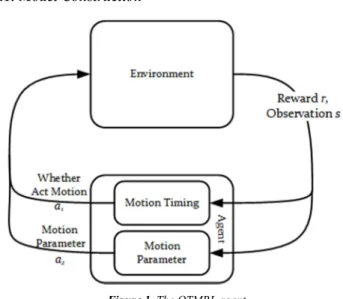
Figure 1. The OTMRL agent.
determines whether to act motion at the current moment according to the current state (observation). If do (i.e. 1), a set of motion parameters is given by the MPM. The simulation environment runs step by step according to the action of the agent and returns the state observation at the next moment to the agent. When a simulation episode is completed, reward is returned.
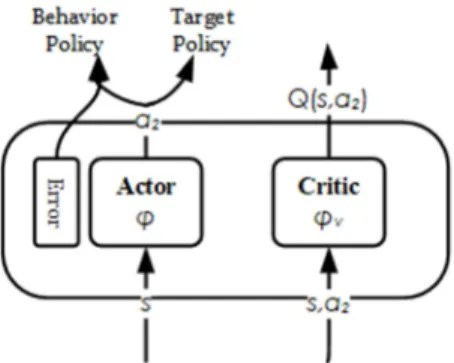
Figure 2. MTM architecture.
3.1.1. Motion Timing Module (MTM)
The motion timing problem is regarded as a discrete control problem in the continuous state space. The MTM has a neural network Actor-Critic structure as Figure 2.
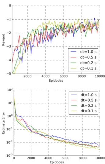
Figure 3. Continuous MPM architecture.
Actor: A three-layer fully connected neural network with parameters denoted by $, and the number of three-layer nodes is the state observation dimension @/, A, 2 respectively. The hidden layer uses the rectified linear unit (ReLU) function as the activation function, and the output layer activation function is a softmax function. The input is the observation . Outputs the probability value B | of whether to act a motion at this moment.
Critic: A neural network with parameters denoted by $C, contains a fully connected hidden layer using ReLU activation functions, and a linear output layer with a single output node. Input the observation , output the state value 2 of .
The Actor network determines whether the action should be performed at each moment according to the input state . The Critic network computes its return estimates 2 to the given state under current policies. The Critic network is used for evaluating the merits of the action according to the state before and after the action , to adjust the Actor parameters $.
3.1.2. Continuous Motion Parameter Module (Continuous MPM)
The continuous motion parameter problem is a continuous
control problem in the continuous state space. We use the DPG method in the MPM whose structure is also Actor-Critic. The structure is shown as Figure 3.
Actor: A neural network with parameters denoted by D fully connected by three layers: input layer, hidden layer, and output layer. The activation function of the hidden layer units is the ReLU function. The output layer activation function is the tanh function, and the output is a continuous variable in the range of 1, 1 . When giving the observation , the motion parameter is calculated. As an off-policy algorithm, with noise is used as the behavior policy action, without noise is used as the target policy action.
Figure 4. Discrete MPM architecture.
Critic: A three-layer fully connected neural network with parameters denoted by DC. The hidden layer uses the ReLU function as the activation function. The output layer unit is a linear activation unit. The network estimate the return
, by the observation s and the motion parameter . The Actor network decides the motion parameter according to the input state . A noise is added on the Actor’s output for better exploration. There are two purposes of training the Critic network. One is to estimate the rewards by choosing in state s to optimize behavioral policies. Another is to provide return estimates for the MTM learning progress.
3.1.3. Discrete Motion Parameter Module (Discrete MPM) As shown in Figure 4, we use the Q-learning method with artificial neural network approximation in the MPM for the discrete motion parameter problem.
The Q network is a three-layer fully connected neural network with parameters denoted by D, which contains a hidden layer using ReLU activation functions, and a linear output layer. The Q network fits the return of motion parameter on the input state . The target policy action is the corresponding motion parameter of the Q network’s maximum output node. For exploration, the MTM uses
-greedy policy as the behavior policy.
3.2. Model Mechanism
reinforcement learning method, which learn policy with current policy experience. Motion parameter module uses an off-policy DPG method, which can make full use of historical experience to converge rapidly. The two modules are not completely independent of one another and need to be coordinated carefully. This section describes the coordinate mechanism.
3.2.1. Operational Mechanism of MTM
Initialize the simulation environment. In each step, the MTM Actor decides with . If 0, the agent won’t act any motion at this moment, and then it would get a new observation . If 1, the MPM Actor decides with . The agentwould act a motion with parameter , and then the episode would terminate with reward .
3.2.2. Operational Mechanism of Motion Timing Module Critic: Update $C using TD method. The policy and the value function are updated after every FGHIJK time-step or when a terminal state is reached. If FGHIJK takes infinity, it will become a Mont Carlo method. In a one-time motion problem, the agent with non-terminal action won’t get reward. So, To updates in a terminal state after acting a motion, we use the value estimate from MPM as the reward of the last state-action pair; the value of the state @ step before,
5 ;L , can be estimated as L . If the episode has not terminated when updating $C , then 5 ;L can be estimated as L5 ; $C , by the value estimate of current state 5 ; $C . We update $C by gradient descent:
Δ$C=O P;Q /O0R.;0R == 2 5 ; $C − T OQ /O0.R;0R (10)
where, T is estimated by
T = U L5 ; $L , for terminal
C , for non − terminal (11)
Actor: Update the policy referring to the Actor-Critic method. In this problem, the advantage function is
( , ; $, $C = T − 5 ; $C . The update gradient can be
written as
Δ$ = T − 5 ; $C \0log | ; $) (12) Multithreading mechanism: For faster training and realizing stable on-policy reinforcement learning, we apply the asynchronous reinforcement learning framework. Asynchronous actor-learners run in parallel environments to explore separately. Each learner calculates Δ$ and Δ$^, and update the global parameters by
$_`ab-` ← $_`ab-`+ -c adΔ$ef (13)
$C_`ab-` ← $C_`ab-`+ cdg gcΔ$Cef (14)
And then pull the global parameters back to the local parameters:
$ef← $_`ab-` (15)
$Cef← $
C_`ab-` (16)
3.2.3. Operational Mechanism of MPM
The operating mechanism of the MPM is a simplified reinforcement learning mechanism. For a one-time action problem, an episode will terminate after the motion parameter module gives the action parameters. Whether the motion parameter space is continuous or discrete, there is no need for TD calculation, because the value of the state-action pair is equal to the reward obtained at the next moment.
For continuous MPM, we update DC by
ΔDC= ∇iR( − 5( , ; DC)) (17)
In this equation, is the actual return of { , }, independent with policies, environment or other factors. Therefore, DC tends to converge quickly.
As to policy function learning, we tune D to maximize the expected return 5 ( , j ( ; D); DC).
ΔD = ∇i 5( , j( ; D); DC) (18)
For discrete MPM, we update D by reduce the Q value estimation error.
ΔD = ∇i ( − ( , ; D)) (19)
Both DPG and DQN are off-policy reinforcement learning algorithm that can learn from the experience not produced by the current behavioral policy. During interacting with the environment, state, action and reward are stored in the form of triples in the Memory. With samples chosen randomly from the memory, MPM parameters are trained with stochastic gradient ascent algorithm.
3.2.4. Learning Procedure See Pseudocode 1. Pseudocode 1 OTMRL
Initialize thread step counter ← 1 Initialize global step counter k ← 1 repeat
Reset gradients: ∆$ ← 0 and ∆$C← 0.
Synchronize thread-specific parameters $’ = $ and $’C= $C
nJIoJ=
Get state repeat
if = 0 according to policy ( | ; $) Perform no motion
else
Perform a motion with parameter according to policy
p( | ; D)
Receive reward , restore < , , > in memory Update D and DC with memory
Calculate expected reward r with the MPM target policy. end if
Receive new state + 1 ← + 1
k ← k + 1
until terminal or − / -d = sIt
U 5 , $ for terminal
C for non-terminal //Bootstrap fromlast state
for x ∈ ' 1, . . . nJIoJ+ do
Accumulate gradients
wrt $: ∆$ ← ∆$ h$’log g| g; $ T 5 g; $C
Accumulate gradients wrt $C’: ∆$C ← ∆$C
∂ T 5 g; $ / ∂$
end for
Perform asynchronous update of $ using ∆$ and of $C using ∆$C.
until k r ksIt
4. Aircraft Bombing Problem
Although one-time motion is common in the real world, there is no simulation environment can be used to test algorithm directly. So we built an aircraft bombing environment for algorithm testing.
The problem of aircraft bombing can be described as follows: the aircraft flies to the target area, and the timing of the bombing and the direction of the bomb dropping are decided during the uniform linear flight. The goal is to make the impact point as close as possible to the specified target point. For easy to understand and discuss, we define the bombing parameters as the relative position of the impact point and the projectile position.
We designed two types of one-time motion problem. The first type is the problem with continuous bombing vector space. For example, in example 1, the bombing parameters can take any two-dimensional vector with a length less than 1. In this problem, the best policy is to drop the bomb toward the target point in a distance less than 1 from the target point. If the closest distance between the route and the target point is greater than 1, the best policy is to drop with the maximum vector toward the target point at the closest point in the track. The other type is the problem with discrete bombing vector parameter space, that is, the bombing parameters can only be selected from several vectors.
In order to formalize aircraft bombing into reinforcement learning tasks, we define a four-dimensional state space B, 2 , where B is a two-dimensional vector of the aircraft position, whose value range is in a circle centered on
0,0 , and 2 is a two-dimensional vector of aircraft speed, a unit vector with arbitrary direction. At each decision-making moment, whether to drop a bomb at this moment should be decided, written as (a 0-1 variable). If “yes”, the bombing parameter should also be given. We define two aircraft bombing problems, named them the continuous bombing parameter space ' + = '∥ ∥q1+ problem and the
discrete bombing parameter space
' + ' 1,0 , 1,0 , 0, 1 , 0, 1 + problem. The observation ~ is equal to the actual state plus error •. The reward is always zero, except in the end of the episode, it is the negative distance between the dropping point and the target point, i.e. B . The episode will terminate in two cases, one is that the aircraft performing a bombing action, and the other is that the aircraft flying out of the bombing area.
5. Experiment
The initial position of the aircraft in the experiment is randomly set in an annulus whose center is at the origin, with an inner radius of 4 and an outer radius of 10. The flight direction is toward a point randomly chosen on a circle centered on the origin with a radius of 1. The aircraft speed is set to 1.
5.1. The Continuous Motion Space Problem
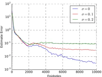
Figure 6. Performance curves for OTMRL in different observation error.
First, we tested the cases with no observation error. The decision-making step length takes various values. The error of observation ~ is set to • 0, and the delay from the observation to the execution of the action is set to 1.5 s. The reinforcement learning tasks are run using an agent composed with the MTM and the Continuous MPM in step length of
d =0.1 s, 0.2 s, 0.5 s, and 1 s, respectively. As shown in Figure 5, the agent can always learn a near optimal policy in 10,000episodes.
Figure 7. Comparison of Discrete OTMRL and A3C.
However, the MTM’s optimality is not as good as the MPM which can quickly converge to the optimal policy. The reason for the high accuracy of the MPM convergence is that the sample distribution is concentrated and the return value is not uncertain. The logic behind the MTM is more complicated. The optimal policy is that the probabilities of executing motion before the optimal timing are 0, and the probability at the optimal timing is 100%. While, on the one hand, learning to adjust the neural network parameters will affect the policies in the entire space, making it impossible to converge to a complex step function. On the other hand, judging whether it is the optimal timing requires learning in the trial and error of reinforcement learning, and the approximation and self-expansion error in learning bring difficulties to learning
the optimal timing.
In the condition of d =0.1 s, we set the observation errors to • = 0,0.1,0.2. The errors of the estimation network are shown in Figure 6. This also has an impact on the optimal timing of the action and parameters. However, policies can still converge to a near optimal one within 10,000 simulations, as shown in Figure 5. It shows that the OTMRL method is robust to observed noise.
5.2. The Discrete Motion Space Problem
We use the agent composed of the MTM and the Discrete MPM to learn the task and compare it with the A3C algorithm. The experimental results are shown in the Figure 7. Both the two methods can converge to an approximate optimal policy, while A3C requires more learning times to converge than the method proposed in this paper. We believe that the main reason may be that A3C treats doing nothing and executing motion with a set of parameter equally. Its policy exploration is blinder.
This structure conforms to the general idea of complex control—hierarchical decomposition. For the control of the one-time action, since the episode is terminated as soon as the action is performed, the sample accumulated by the MPM memory can accurately reflect the action value, and the evaluation network can generally converge quickly.
6. Conclusion
Because both the timing and action parameters of the motion are important, methods with manually splitting the control element will cause problems. The OTMRL method combines the motion timing decision of 0-1 variable with the motion parameter decision of continuous variable to optimize together and realize fast and stable convergence to an optimal policy.
Reinforcement learning is currently the only machine learning method that can directly learn optimal control (function extreme value problem). However, the convergence of reinforcement learning to continuous functional has not been proved, and the method of adjusting parameters has not been fully studied.
The design of the reward function, the inherent difficulty of this reinforcement learning, will have an important impact on the OTMRL learning. The basic requirement for the design of reward functions is that there is a learnable gradient in the state space. In this problem, on the one hand, the closer the point is to the target point, the larger the reward, on the other hand, the modulus of the action parameter is used as a penalty factor to avoid the gradient disappearing within the large optimal action timing, resulting in instability of policies.
step size is, the smaller the difference in returns between adjacent steps, which makes it impossible to converge to the optimal policy.
Acknowledgements
This work was supported in part by the National Natural Science Foundation of China under Grant 61403397 and Grant 61202332.
References
[1] Wen-yan Pang. Optimal Output Regulation of Partially Linear Discrete-Time Systems Using Reinforcement Learning. CPCC 2019. 2019: 252.
[2] J. Jabłońska, Ł. Szumiec, J. R. Parkitna. Reinforcement learning in a probabilistic learning task without time constraints. Pharmacological Reports. 2019, 71 (6).
[3] Paulo C. Heredia, Shaoshuai Mou. Distributed Multi-Agent Reinforcement Learning by Actor-Critic Method. IFAC Papers On Line. 2019, 52 (20).
[4] V. Mnih, K. Kavukcuoglu, D. Silver, A. A. Rusu, J. Veness, M. G. Bellemare, A. Graves, M. Riedmiller, A. K. Fidjeland, G. Ostrovski. Playing Atari with Deep Reinforcement Learning. Nature. 518 (7540), 529 (2015).
[5] D. Silver, A. Huang, C. J. Maddison, A. Guez, L. Sifre, d. D. G. Van, J. Schrittwieser, I. Antonoglou, V. Panneershelvam, M. Lanctot. Human-level control through deep reinforcement learning. Nature. 529 (7587), 484 (2016).
[6] Zhen-peng Zhou, K. Steven, Li Li, Z. Richard N, R. Patrick. Optimization of Molecules via Deep Reinforcement Learning. Scientific reports. 2019, 9 (1).
[7] G. A. Rummery, M. Niranjan. On-line Q-learning using connectionist systems. vol. 37 (University of Cambridge, Department of Engineering Cambridge, England, 1994). [8] R. S. Sutton. Generalization in Reinforcement Learning:
Successful Examples Using Sparse Coarse Coding. in International Conference on Neural Information Processing Systems (1995). pp. 1038–1044.
[9] C. J. C. H. Watkins, P. Dayan. Q -learning. Machine Learning. 8 (3-4), 279 (1992).
[10] V. Mnih, K. Kavukcuoglu, D. Silver, A. Graves, I. Antonoglou, D. Wierstra, M. Riedmiller. Playing Atari with Deep Reinforcement Learning. Computer Science (2013).
[11] R. S. Sutton, A. G. Barto. Reinforcement learning: An introduction (MIT press, 2018).
[12] R. J. Williams. Simple statistical gradient-following algorithms for connectionist reinforcement learning. Machine Learning. 8 (3-4), 229 (1992).
[13] I. H. Witten. An adaptive optimal controller for discrete-time Markov environments. Information & Control. 34 (4), 286 (1977).
[14] Sutton, Richard. Temporal credit assignment in reinforcement learning. Phd Thesis University of Massachusetts. 34 (5), 601 (1984).