An Online Compression Algorithm for Positioning Data Acquisition
Wei Pan, Chunlong Yao, Xu Li and Lan Shen
School of Information Science and Engineering, Dalian Polytechnic University, Dalian 116034, China E-mail: [email protected]
Keywords: location data acquisition systems, positioning data, trajectory compression, trajectory recovery
Received: September 17, 2014
Positioning data are usually acquired periodically and uploaded to the server via wireless network in the location data acquisition systems. Huge communication overheads between the terminal and the server and heavy loads of storage space are needed when a large number of data points are uploaded. To this end, an online compression algorithm for positioning data acquisition is proposed, which compresses data by reducing the number of uploaded positioning points. Error threshold can be set according to users’ needs. Feature points are extracted to upload real-timely by considering the changes of direction and speed. If necessary, an approximation trajectory can be obtained by using the proposed recovery algorithm based on the feature points on the server. Positioning data in three different travel modes, including walk, non-walk and mixed mode, are acquired to validate the efficiency of the algorithm. The experimental results show that the proposed algorithm can get appropriate compression rate in various road conditions and travel modes, and has better adaptability.
Povzetek: Predstavljen je nov algoritem za zajemanje podatkov o realnem času, uporaben za sisteme za določanje položaja.
1
Introduction
With advances in tracking technologies and the rapid improvement in location-based services (LBS), a larger amount of location data needs to be collected [1]. These positioning data are linked up in chronological order to form a trajectory which contains a sequence of positioning data with latitude, longitude and timestamp. Trajectory can be used for positioning, navigation, providing some location-based services and expressing
user geospatial history behaviour. For location
acquisition systems, a large number of positioning data not only generate lots of communication overheads but also bring heavy burden for the storage system [2]. A major reason for this problem is that the uploaded data points are far more than necessary points [3]. Therefore, trajectory compression and simplification have received increasing concern.
Trajectory compression can be classified into two categories, offline compression and online compression. In the offline compression, all data points collected (usually on the server) are considered for compression regardless of the data transfer process. In the online compression, data points are processed before they are uploaded, and only feature points selected are transmitted to the server.
For the offline compression, Zhang et al. [2] proposed a trajectory data compression algorithm based on the spatial-temporal characteristic. In order to extract
accurately trajectory information, the algorithm
calculates the distance standard to judge the feature point according to the three-dimensional spatial-temporal characteristic of GPS data points. Given a trajectory Traj and error threshold, the Doulas-Peucker Algorithm [4]
constructs a new trajectory Traj’ by adding points from
Traj repeatedly until the maximum spatial error of Traj’ becomes smaller than error threshold. The Douglas-Peucker algorithm has the limitation of ignoring temporal data. Top-Down Time Ratio (TD-TR) [5] overcomes this
limitation by using Synchronized Euclidean Distance
(SED) [6] instead of spatial error. The characteristics of the vehicle trajectory are described in the proposed algorithm [7], in which the advantages and disadvantages of judgment method with point by point and judgment method with multi-point joint are analysed. This algorithm puts forward the description method for trajectory based on turning point judgment method. Chen et al. [8] proposed a trajectory simplification algorithm (TS), which considered both the shape skeleton and the semantic meanings of a GPS trajectory. The heading change degree of a GPS point and the distance between this point and its adjacent neighbours in this algorithm are used to weight the importance of the point. By studying the model of temporal data in vehicle monitoring system, Wang et al. [9] proposed a modelling idea for establishing trajectory version. To reduce storage and improve temporal queries, spatial-temporal cube is segmented to form unit spatial-temporal cube by this modelling idea. With discussing some problems of trajectory data compression about road net, Guo [10] proposed a non-linear compression algorithm of moving objects trajectories based on road net.
between the terminal and the server are huge and burdens of storage space are heavy. In recent years, some online compression algorithms have been proposed.
Similar to Douglas-Peucker, Opening Window algorithm [11] approximates each trajectory using an increasing number of points so that the resulting spatial error is smaller than the bound. This algorithm is a generalized online compression with a little delay, and it works without considering time data. Opening Window Time Ratio (OPW-TR) [5] is an extension to Opening Window which uses SED instead of spatial error. Compared to Opening Window algorithms, OPW-TR has the benefit of taking temporal data into account. However, just like Opening Window algorithm, OPW-TR also has a little delay. Both of them cannot real-timely determine whether current point needs to be compressed. An algorithm called SQUTSH (Spatial QUalIty Simplification Heuristic) [12] uses a priority queue where the priority of each point is defined as an estimate of the error that the removal of that point would introduce. SQUISH compresses each trajectory by removing points of the lowest priority from the priority queue until it achieves the target compression ratio. This algorithm is fast and tends to introduce small errors during compression. However, it cannot compress trajectories while ensuring that the resulting error is within a user-specified bound. It also exhibits relatively large errors when the compression ratio is high [13]. Yin et al. [14] proposed an algorithm and a restraining model for vehicle data stream transmission. It gives a formula for data recovery in the monitoring centre by discussing the determination condition of speed and direction change degree in the algorithm. However, this algorithm is suitable for the integrated system of monitoring and navigation, and must be matched to the map. Wang et al. [15] proposed an improved moving object model based on vehicle monitoring system of moving objects model. This model provides a dynamic time selection algorithm, which adjusts dynamically the time density according to object moving speed. Therefore, the number of communications is reduced effectively. However, this algorithm works regardless of data recovery and the issue that the moving direction affects the accuracy of the model. Han et al. [16] proposed an adaptive algorithm for vehicle GPS monitoring data. The speed function is expressed by using fitting polynomial with constraint based on endpoint speed and mileage. This algorithm considers the case that terminal with and without map, in which the deviation distance is used for denoting the deviation of speed direction. At the same time, data recovery algorithm, algorithm evaluation index and application mode of algorithm are proposed in this algorithm. However, it must be set speed threshold in advance according to the road. In practice, according to the different road, predetermined speed threshold is very difficult.
In this paper, an online compression algorithm for positioning data acquisition systems is proposed, which compresses the data points before transmission from terminal to the server. In this algorithm, the feature points are extracted and uploaded by computing the
change of speed and direction based on error threshold
set according to the users’ requirements, and non-feature
points are discarded to reduce unnecessary data transmission and bandwidth occupation.
The remainder of this paper is organized as follows. Section 2 describes our new online compression algorithm for positioning data acquisition in detail. An experimental evaluation of trajectory compression algorithm is provided in Section 3. The paper concludes with future work in Section 4.
2
The online compression algorithm
In order to compress an original trajectory, the key of our algorithm is to pick out feature points .For each point collected in the terminal, the current point will be uploaded and preserved if it is a feature point, else it will be discarded as a non-feature point. If needed, the recovery trajectory that approximated to the original trajectory can be obtained by the recovery algorithm with the feature points on the server. Our algorithm involves feature points, non-feature points and lost points. A feature point is a positioning point that a large change in speed or direction; a non-feature point is a positioning point that is discarded with a small change in speed and direction; a lost point is a positioning point that is lost because the communication delay caused by the positioning signal blind area. Generally, original trajectory is a temporally ordered sequence of positioning
points P = {p1, p2, …, pn}, for i = 1, 2, …, n, pi = (lngi ,
lati, ti) where lngi, lati represent the longitude and latitude of the ith point and ti stands for the time stamp. For a point pi, pi.lng, pi.lat and pi.t denote longitude, latitude
and time stamp of pi respectively. For each positioning
point pi in an original trajectory, recovery point pi’of pi is
a data point obtained by the recovery algorithm, which
represents piin the recovery trajectory.
2.1
Algorithms
In the compression phase, error threshold and acquisition interval are set in advance according to accuracy requirements. The initial two collected points (these two points must be the feature points) are directly uploaded to the server without judgment. Starting from the third positioning point, corresponding recovery point is calculated for each point collected currently. The distance between the actual point pi and its corresponding
recovery point pi’is compared with the error threshold. If
p2
p5
p4
p3
pk p
i
p3’ p4’
pk-1’
pk-1
pi’
d3 d4
dk-1
di
d5
´
...
... ...
p1
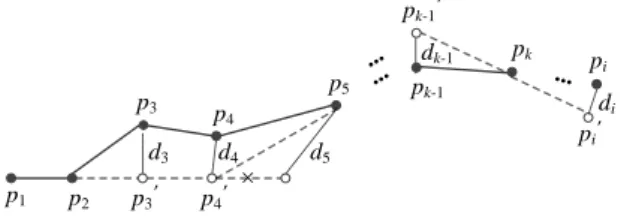
Figure 1: A schematic diagram for the compression process.
As shown in Fig. 1, p1, p2, p3, p4, p5, pk-1, pk and pi
are the original positioning points, each positioning point
has a corresponding recovery point. p1, p2, p5 and pk are
feature points, their recovery points are themselves. p3’,
p4’and pk-1’are recovery points of p3, p4 and pk-1. p2 is
previous feature points of p3’and p1 is previous points of
p2. p3’is calculated by p1 and p2. The speed of p2 can be
concluded by distance and time d-value between p1 and
p2. Supposing p2 and p3’have the same speed. The
product of this speed and interval T is the distance of p3’.
Set p3’on a straight line that p1, p2 are located at.
According to the coordinate of p1 and p2, the coordinate
of p3’can be calculated. In the same way, p2 is still
previous feature points of p4’ and p5’, and they are also
calculated by p1 and p2. Differently, the distance of p4’ is
the product of speed of the p2 and twice interval T, the
distance of p5’is the product of speed of the p2 and triple
interval T. The distance between recovery point pi’ and
actual point pi is called di and di is compared with the
error threshold D. If di ≥ D, current point is uploaded as a feature point. If not, current point is discarded as
non-feature point. d3, d4 in Fig. 1 are smaller than D, so p3, p4
are discarded. d5 is not less than D, so p5 is uploaded as
feature point. The recovery point pi’ of current point pi is
calculated though the previous feature points pk of pi
’and the previous point pk
-1’ (it can be a feature point
or not) of pk. The speed of pk is calculated according to pk
and pk-1’. The product of this speed and time d-value
between pi and pk is the distance of pi’. Set pi’in the
straight line that pk, pk-1’are located at. According to the
coordinate of pk, pk-1’ and the distance of pi’, the
coordinate of pi’ is calculated. In the recovery phase,
p1, p2, p5 and pk are recovered directly as feature points.
p3, p4 and pk-1 are non-feature points. They are recovered
to p3’, p4’, pk-1’ according to the above process.
In the recovery phase, the first and second feature points received are recovered directly. Determine whether there are non-feature points between the current
piand previous feature point pkfrom the third feature
point. If there are non-feature points, they are recovered in order by calculating corresponding recovery points according to pk. Then recover the current point pi after all
non-feature points between pi and pk are recovered.The
process cycles until the recovery of the last feature point. To deal with the problem of lost point, positioning point pi introduces lost point count (Count) property and it is given with pi = (lngi, lati, ti, ci). The design idea is to add a counter in the terminal. Positioning data are
collected at an interval. This interval is consistent for counter and data acquisition. When the time reaches an interval, if the signal is acquired, the counter is "0". If the signal is not acquired, that is the signal loss, counter is added with "1" until the signal is acquired. Fig. 2 shows a
schematic diagram for the lost point
.
p2 p3’ p1
p4 p5
... pi
Figure 2: A schematic diagram for the lost point.
As shown in Fig. 2, p1, p2 and p4 are original
positioning points. After compression, p3 is discarded as
non-feature point and p3’is corresponding recovery point
of p3. There are three intervals between p3 and p4, and it
should have two positioning points between them. However, due to signal loss, these two points are not collected. They are called the lost points. When
determining whether p5 is a feature point or not, p3’and
p4 are made use for calculation direct without considering
the lost points. When recovery of p3’, the lost points are
needed to consider. There are four intervals between two
feature points p2 and p4. It should have three positioning
points. Since C4 = 2, that is to say, two positioning point
are lost, so just to recover the only non- feature point p3.
2.2
Algorithm description
The recovery point is used to determine whether the current point is a feature point in the compression phase. The recovery point is the non-feature point recovered in the recovery phase. Therefore, the calculation of recovery point is the key of the algorithm. Making use of
the previous feature point pk of pi’and the previous point
pk-1’of pk to calculate the recovery point pi’of current
point pi (if i = 3, then pk = p2,pk-1’= p1).
2.2.1 The compression algorithm
The recovery point of current point is calculated from the third positioning point collected. The actual point has attributes of latitude and longitude. For ease of calculation, latitude and longitude as spherical coordinate can be transformed into rectangular coordinate by the
algorithm [17]. That is to say, pi= (longi, lati, ti) as
spherical coordinate is transformed into pi = (xi, yi, ti) as
rectangular coordinate. For any two points pi and pj, the
distance of them is Lj= Dist (pi, pj) in the trajectory with n points. Accordingly, the distance between pk and pk-1’is
Lk. pk and pk-1’are the consecutive points and the time
d-value of them is pk. t - pk - 1’.t (in the case of signal not
loss, the d-value is the interval T). The speed Vi is
calculated by Formula (1) and interval T. The distance Si
of pi’is calculated according to the time d-value of pi, pk
Lk=Dist(pk1,pk)
= ( . . ) ( . 1. )2, 2 1
2
1
p x p y p y k n
x
pk k k k (1)
Vi =
t
p
t
p
L
k k k.
.
1
= p t p t k n-, i ny p y p x p x p k k k k k
k
3 1 2 , . . ) . . ( ) . . ( 1 2 1 2 1
(2)
Si = Vi´ (pi.tpk.t)
= p t p t k n-, i n
t p t p y p y p x p x p k i k k k k k
k ´
3 1 2 ), . . ( . . ) . . ( ) . . ( 1 2 1 2 1
(3)
After calculating the distance of pi’, position
coordinate of pi’ is calculated according to rectangular
coordinates of pk and pk-1’and triangle similar properties
[18]. Formulas are as follows. Detailed compression
process is shown in Algorithm 1.
pi’.x = pk.x +
k k k i
L
x
p
x
p
s
´
(
.
1
.
)
= pk.x + , 2 1 3
. . ) . . ( ) . . ( 1
1 k n-, i n
t p t p x p x p t p t p k k k k k
i
´
(4)
pi’.y = pk.y +
k k k i
L
y
p
y
p
s
(
.
1.
)
´
= pk.y + k n-, i n
t p t p y p y p t p t p k k k k k
i
´
, 2 1 3
. . ) . . ( ) . . ( 1
1 (5)
2.2.2 The recovery algorithm
Determine whether exist the non-feature points between
the current point pi and the previous feature point pk
from the third feature point received. Judgment is that getting the number Ni of intervals based on the time
d-value of two points divided by the interval T. By the
Formula (6) and the number Ci of lost points pi, the
number Mi of recovery point is calculated. Special
attention is that the interval number of two adjacent original positioning points is “1”, but there is no recovery point between them. Therefore, the number of
Algorithm 1 for compression
Input: pi , pk andpk-1’, D and T.
Output: A simplified trajectory Traj’ with feature points.
1. Collect data points and open counter , Traj’ = Φ;
2. Upload p1 and p2; // The first and second positioning point needn't decide and are uploaded directly
3. pk = p2 ,pk-1’= p1; //p2 is assigned to pk, p1 is assigned to pk-1’
4. Foreach pi (i ≥ 3); //Cyclic judge for pi
5.Transform pi = (lngi, lati, ti) to pi = (xi, yi, ti); // Spherical coordinate is transformed into rectangular coordinate 6. Calculate Si; // Calculate the distance of pi’
7.Calculate (xi,yi); // Calculate the rectangular coordinate of pi’
8.Transform pi = (xi, yi, ti) to pi = (lngi, lati, ti); // Rectangular coordinate is transformed into spherical coordinate 9. Dist(pi,pi’) is di; // The distance of pi and pi’ is di
10. Compare di and D ; // Error threshold is D
11. If(di ≥ D), upload pi; // If di ≥ D,upload pi as a feature point
12. pk = pi , pk-1’= pi-1’; // pi assigned to pk,pi-1’ assigned to pk-1’
13. Else(di < D), ignore pi; // If di < D,discard pias a non-feature point
14. End foreach; // End of cycle
15. Return Traj’ = {p
recovery points should extra minus “1”. If Mi is not equal“0”, it means that it exists recovery points. To recover the Mi recovery points in order. The speed of the recovery point is calculated by Formula (2), and the
product of speed and r interval T is the distance Gr of
the r-th recovery point.
Ni = T
t p t pi. k.
, 3 ≤ i ≤ n, 2≤ k ≤n-1 (6)
Mi = Ni - Ci -1, 3 ≤ i ≤ n (7) Gr = Vi ´ r ´ T, 3 ≤ i ≤ n, 1 ≤ r ≤Mi (8) After calculating the distance of each recovery point, the position coordinate of each recovery point is calculated according to rectangular coordinate of pk and
pk-1’, triangle similar properties and Formula (4), (5).
Detailed recovery process shown in Algorithm 2.
Compression algorithms can be divided into lossless and lossy compression. Lossless compression enables exact reconstruction of the original data with no information loss. In contrast, lossy compression introduces inaccuracies when compared to the original data. Lossy compression allows the compression process to loss some information. Although we cannot fully recover the original data, but the lost part has a smaller impact on the understanding of the original data, at the same time, in exchange for a smaller compression rate [19]. The primary advantage of lossy compression is that it can often reduce the storage requirements drastically while maintaining an acceptable degree of error [20]. Although all compressed data are recovered by the algorithm proposed in this paper, but it has a certain geographical deviation, so that this algorithm is lossy compression.
3
Experiments
To verify the applicability and performance of the algorithm, a large number of experiments are performed about original data acquisition, data compression and data recovery real-time by PC and GPS phones.
3.1
Experimental environment
The existing four global satellite navigation system in the world, namely the U.S. GPS system, China Beidou system, the European Galileo system and Russia GLONASS system [21]. GPS system is widely used because of its wide coverage, high positioning accuracy, short positioning time and small location-dependent and
other advantages. Positioning data are collected real-timely with Android operating system and GPS positioning system in the experiment. Android includes API libraries that simplify the development related to the device hardware. Android SDK includes location-based services, and determines the current location by GPS.
The mobile phone is used as terminal in the experiment, which is regarded as a GPS receiver and a compression processor for positioning data. The PC is used as server, which is used for receiving positioning data compressed, and recovering the original trajectory based on those data.
3.2
Select the experimental route
The actual movement broadly divided into walk, non-walk (car, bicycle, aircraft, ships, etc.) and mixed mode (alternating walk and non-walk) according to different travel modes. According to different speed, it can be
broadly divided into 0-30 km/h as the low-speed
movement (walking, jogging, bicycle, etc.), 30-60 km/h as the middle-speed movement (low speed vehicles,
etc.) and 60 km above as high-speed movement (cars,
boats, airplanes of high speed, etc.). Assuming the original trajectory with n positioning points, the purpose of the experiment is to select as few as m feature points.
When m < n, compression trajectory is constituted with
m feature points. Set r = m / n is the compression rate, the r is the smaller the better without changing the original shape of the trajectory of geography. For moving at different speed and different travel modes, it should set a different error threshold. In this paper, the
Algorithm 2 for recovery
Input: Feature points and T.
Output: Arecovered trajectory Traj with feature points and recovery points.
1. Receive feature points and Traj= Φ;
2. Recover p1 and p2,Traj = {p1, p2}; // The first and second feature points are recovered directly without deciding
3. pk = p2 , pk-1’= p1 ; // p2 is assigned to pk, p1 is assigned to pk-1’
4. Foreach pi (i ≥ 3); // Cyclic judge for current feature point pi
5.Calculate Mi ; // Calculate the number of recovery points between current feature point and previous feature point 6. Foreach r (1≤ r ≤ Mi ); // Cycle begins from 0 to Mi non-feature points
7.Transform pi = (lngi, lati, ti) to pi = (xi, yi, ti); // Spherical coordinate is transformed into rectangular coordinate 8.Calculate Gr ; // Calculate the distance Gr of current recovery point
9.Calculate (xi, yi); // Calculate the rectangular coordinate of current recovery point
10.Transform pi = (xi, yi, ti) to pi = (lngi, lati, ti); // Rectangular coordinate is transformed into spherical coordinate 11. Recover recovery points ; // Recover recovery points
12. Recover pi ; // Recover current feature point pi
13. pk = pi, pk-1’= pi-1’; // pi is assigned to pk, pi-1’ is assigned to pk-1’
14.End foreach; // End of the cycle
experiment is given priority to low speed movement, and divided into walk, non-walk and mixed mode for validation. Data is acquired at 2s intervals, 5s intervals, 10s intervals and 20s intervals. For each acquisition interval, 5m, 10m, 15m, 20m and 25m as the error threshold are set for compression.
In this experiment, the actual routes as an example are shown in Fig. 3. Positioning data acquisition,
compression and recovery are executed real-timely. Fig. 3a) shows a route of non-walk (by bus) and mixed mode (by bus and walk); Fig. 3b) shows a route of walk. Due to traffic restrictions, travel by bus is slow. So this experiment is under the condition of low-speed movement.
a) The route of non-walk (by bus) and b) The route of walk
mixed mode (by bus and walk)
Figure 3: A schematic diagram for actual routes.
3.3
Experimental results and analysis
3.3.1 Effects of different parameters on the
compression rate
In the actual routes shown in Fig. 3, the compression rate is impacted by the acquisition interval, the error threshold and the travel mode.
Under the conditions of the error threshold are 5m, 10m, 15m, 20m and 25m, and the travel mode is walk, the effect of different acquisition intervals on compression rate is shown in Fig. 4.
Figure 4: Compression rate of different acquisition intervals.
The Fig. 4 shows that, for the walk of low-speed movement, the shorter the acquisition interval is, the more positioning data are compressed and the smaller the compression rate is. At the same time, we can draw that data compression rate decreases with increasing error threshold. That is to say, the bigger threshold is set, the more data are discarded and the smaller the
compression rate is. With the increasing of the
threshold, it also brings the risk of losing detailed information.
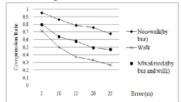
Under the conditions of the error threshold are 5m, 10m, 15m, 20m and 25m, and the acquisition interval is 10s, the effect of different travel modes on compression rate is shown in Fig. 5.
Figure 5: Compression rate of different travel modes
The Fig. 5 shows that for low-speed movement, walk on the relatively straight route without more detours and its speed is more even, so it has the minimum compression rate at the same error threshold. Non-walk is on the route with more detours and it is ongoing to stop and go, at the same time, the change degree of speed is bigger, so it has the maximum compression rate at the same error threshold. Mixed mode includes walk and non-walk, so the compression rate ranges between them.
3.3.2 Effectiveness
The recovery trajectory is compared with the original trajectory to verify the effectiveness of
proposed algorithm. The recovery trajectory
a) Original trajectory b) Compression trajectory c) Recovery trajectory
Figure 6: A schematic diagram for original trajectory, compression trajectory and recovery trajectory.
The Fig. 6 shows a schematic diagram for original
trajectory, compression trajectory and recovery
trajectory of walk under the conditions of acquisition interval is 10s and the error threshold is 10m. Fig. 6a) shows the original trajectory with 112 points; Fig. 6b) shows the compressed trajectory according to the online compression algorithm for positioning data acquisition with 42 points; Fig. 6c) shows the recovery trajectory by recovery algorithm with 112 points, the same number as the original data, recovery trajectory approximates original trajectory. That is to say, the compression rate is 37.5%, and denser data are discarded. In addition, the spatial error of points recovered is strictly controlled under the error threshold. The above fact shows that the proposed algorithm is effective in practical applications. The deviation of a recovery trajectory depends on the error threshold predetermined. The larger error threshold is set, the more non-feature points are compressed, the compression rate is smaller, but the deviation between original data and recovered data is larger. Conversely, the smaller error threshold is set, the less non-feature points are compressed, the compression rate is larger, but the deviation between original data and recovered data is smaller, the recovered data are more approximate to the original data.
4
Conclusion
In this paper, an online compression algorithm for positioning data acquisition is proposed based on a straight line approach. Considering the change of speed and direction, the error threshold between the actual point and recovery point is set, as the required accuracy of user, to replace the threshold of speed or direction. As a result, the feature information loss and trajectory error can be significantly reduced. The algorithm is suit for different road conditions and travel modes, so it has a better adaptability than the existing compression algorithm. In the future, one possible approach for improving the compression of positioning data would be to use knowledge of the road network. This approach would require fast detection of deviations from the road network. A key goal in this approach is that enable a smaller compressed representation with low calculating overhead and reduced error.
References
[1] Choi, D.Y. (2007) “Personalized local internet in
the location-based mobile web search”, Decision
Support Systems, Vol.43 No.1, pp. 31- 45.
[2] Zhang, D.F. and Zhang, X.M. (2013)
“Compression algorithm of GPS trajectories data
based on the temporal characteristics”, Journal of
Transport Information and Safety, Vol. 31 No.3, pp. 6-9.
[3] Kaul, S., Gruteser, M., Rai, V. and Kenney, J.
(2010) “On predicting and compressing vehicular GPS traces”. In: Proceedings of the 2010 IEEE international conference on communications Workshops (ICC Workshops), pp. 1–5.
[4] Douglas, D.H. and Peuker, T.K. (1973)
“Algorithms for the reduction of the number of points required to represent a line or its caricature”, Can Cartogr, Vol.10 No.2, pp. 112–122.
[5] Meratnia, N and de By RA (2004) “Spatiotemporal
compression techniques for moving point objects”, In: Proceedings of the 9th international conference on extending database technology (ED BT), Crete, Greece, pp. 765–782.
[6] Potamias, M., Patroumpas, K. and Sellis, T. (2006)
“Sampling trajectory streams with spatio-temporal
criteria”, In: Proceedings of the 18th international
conference on scientific and statistical database management (SSD BM), pp. 275–284.
[7] Xu, J. and Tian, S.L. (2010) “GPS location data
reducing based on turning point judgment method”, Computer Engineering, Vol.36 No.7, pp. 268 -269 +272.
[8] Chen, Y.K., Jiang, K., Zheng, Y., Li, C. and Yu,
N. (2009) “Trajectory simplification method for Location-Based Social Networking Services”, ACM GIS workshop on Location-based social networking services, pp. 33-40.
[9] Wang, W.J., Weng, J.N. and Fan, K. (2006)
“Design and implementation of spatial-temporal
data model in vehicle monitor system”, Computer
Engineering and Design, Vol.27 No.6, pp. 1042 -1044 +1051.
[10] Guo, Z.Z. (2008) “Compression of moving objects
trajectories based on road net”, Computer and
[11] Keogh, E.J., Chu, S., Hart, D. and Pazzani, M.J. (2001) “An online algorithm for segmenting time
series”, In: Proceedings of the 2001 IEEE
international conference on data mining (ICDM), California, USA, pp. 289–296.
[12] Muckell, J., Hwang, J.H., Patil,V., Lawson, C.T.,
Ping, F. and Ravi, S.S., (2011) “SQUISH: an online approach for GPS trajectory compression”,
In: Proceedings of the 2nd international
conference on computing for geospatial research and applications (COM. Geo), New York, USA, pp. 13.1–13.8.
[13] Muckell, J., Olsen Jr, P.W., Hwang, J.H., Lawson,
C.T., and Ravi, S.S., (2014) “Compression of trajectory data: a comprehensive evaluation and
new approach”, In: Geoinformatica, Vol.18, pp.
435-460.
[14] Yin, J.Z., He F.Q., Li Q.Q. and Xu, L. (2008)
“Data stream transmission control algorithm in navigation and monitoring integrated system”, Geomatics and Information Science of Wuhan University, Vol. 33 No. 9, pp. 900-903.
[15] Wang, S.S. and Liu, D.Y. (2004) “Moving object
model based on vehicle monitor system”, Chinese
Journal of Scientific Instrument, Vol. 25 No.4, pp. 509-511 +524.
[16] Han, X.G., Yan, L. and Lu, W. (2011) “Adaptive
acquisition algorithm for vehicle GPS monitoring
data”, Geography and Geo-Information Science,
Vol. 27 No.3, pp. 12-16.
[17] Yang, P. (2009) “An easy way to convert GPS
coordinates in EXCEL”, Fortune China Science
and Technology , No. 04.
[18] Chen, Y.M., Feng, H.L and Dai, Q.H. (2010) “The
research of Delta grey correlation based on similar
triangle”, Statistics and Decision, No. 23, pp.
16-18.
[19] Yang, H.Y. and Zhang, Y. (2002) “Design and
implementation algorithm of the GPS positioning
data compression”, Application of Electronic
Technique, No.12, pp. 29-32.
[20] Muckell, J., Hwang, J.H., Lawson, C.T. and Ravi,
S.S., (2010) “Algorithms for compressing GPS trajectory data: an empirical evaluation”, In: Proceedings of the 18th SIGSPATIAL international conference on advances in geographic information systems (ACM - GIS), pp. 402–405.
[21] Liu, M.S. (2006) “Global positioning system and
its application(1)—history of development for
navigation and positioning technology”, China