УДК 629.4
G. BUREIKA, Vilnius Gediminas Technical University
R. SUBA
Č
IUS, Vilnius Gediminas Technical University
MATEMATICAL MODEL OF DYNAMIC INTERACTION
BETWEEN WHEEL-SET AND RAIL TRACK
У статті показаний вплив моделюючих параметрів, що враховуються раціональним способом, застосовуючи фракційний факторіал двох рівнів, на розподіл напружень у різних місцях рейки. Представлено аналіз вертикальної динаміки взаємодії твердого колеса з рейкою. З метою мінімізації напружень рейки шукається оптимальний варіант комбінації безлічі параметрів із застосуванням методу фракційногофакторіаладвохрівнів.
Встатьепоказановлияниемоделируемыхпараметров, которыеучитываютсярациональнымспособомс применением фракционного факториала двух уровней на распределение напряжений в различныхместах рельсовогозвена. Представленанализвертикальнойдинамикивзаимодействияжесткогоколесасрельсом. С цельюминимизациинапряженийрельсапроизводитсяпоископтимальноговариантакомбинациимножества влияющихпараметровсприменениемметодфракционногофакториаладвухуровней.
The main goal of this paper is to show how the effects of maximum bending tensions at different locations in the track caused by simultaneous changes of various parameters can be estimated in a rational manner. The dynamics of the vertical interaction between a moving rigid wheel and a flexible railway track is investigated. An asymmetric linear three-dimensional beam structure model of a finite length of the track is suggested. The influence of eight selected track parameters on the dynamic behaviour of the track is investigated. A two-level fractional factorial design method is used in the search for the combination of numerical values of these parameters minimizing the maximum bending tensions.
Introduction
The aim of this paper is to show how the effects on maximum pressure tensions at different locations in the track caused by simultaneous changes of the parameters can be estimated in a rational manner [1, 2]. An accurate mathematical modelling and numerical solution of dynamic interaction problems for vehicles on their tracks were investigated [3–5]. Higher vehicle speeds and axle loads generally lead to the increased magnitudes of dynamic responses (such as deformations, accelerations and tensions) of the track as well as of the vehicle. The interactive forces developed between vehicle and track depend on the dynamic properties of the two and also on the vehicle speed and the initial irregularities along the track and the wheel perimeter. Therefore, a rather comprehensive mathematical model of the compound system including both vehicle and track should be used.
Track models including rails and pads and also flexible sleepers resting on an elastic foundation have earlier been presented in reference [5]. The modelled rail is an infinite beam resting on a uniform support. This support includes three continuous layers on top of each other describing firstly, resilient pads with viscous damping, secondly, sleepers modelled as uniform beams and
thirdly ballast modelled as a viscously damped foundation.
Rails and sleepers were modelled using of Euler-Bernoulli beam elements. The response due to a moving mass with a non-linear Hertzian contact spring traversing a corrugated track was calculated using of time integration and modal superposition with proportional viscous damping added. Field experiments were performed which, according to [6], confirmed the predicted dynamic responses. The same type of track model and the same solution technique were also adopted. The contact force due to a moving wheel-set mass with different irregularities was calculated in [4].
The dynamic interaction between moving rigid wheel-set mass, with a perfectly round and smooth tread, and an initially straight and non-corrugated continuous railway track model was studied in this paper. Some examples including a four degrees-of-freedom wheel-set model on a track model with 40 sleeper bays were given in [5]. Rather comprehensive three-dimensional beam structure model of the track containing rail, pads, sleepers and ballast was developed.
As it was mentioned, the dynamic interaction studied in this paper is restricted to the special case of a single rigid wheel with a smooth peripheral surface traversing an initially straight and non-corrugated track. However, the general solution
technique in [6] allows a great variation of possible loading cases to be studied including a non-linear discretised vehicle model with several degrees-of-freedom on a track with an arbitrary continuous vertical surface profile. Since complex modal synthesis is used, the model of the track structure can be very general (but linear).
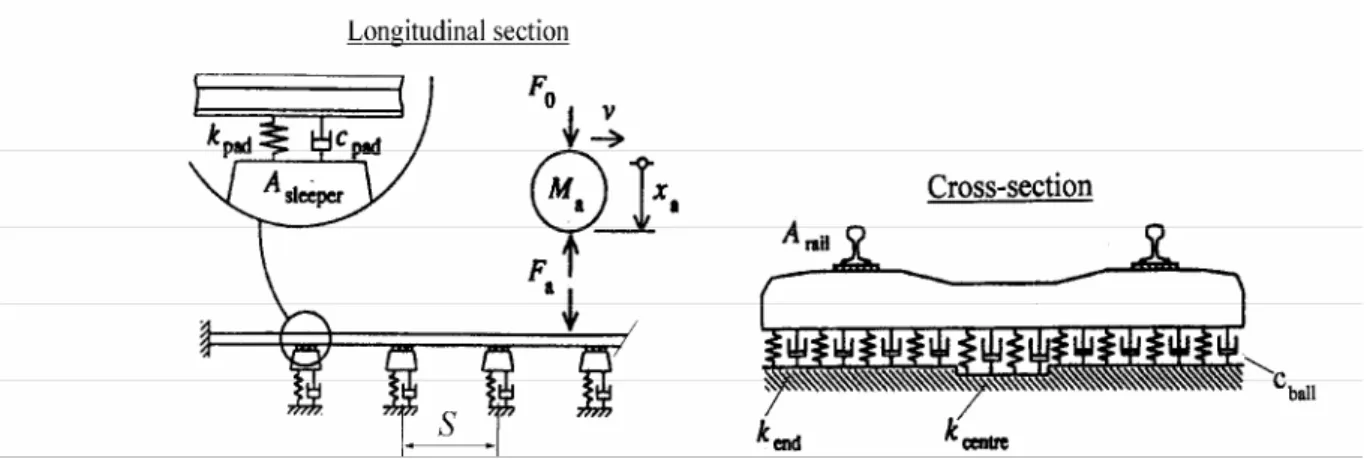
1. Mathematical Models of Track and Wheel-set The mathematical model of a railway track section of finite length (12.5 m) to be used in the numerical theoretical experiments will now be described. It consists of 25 sleepers bays as shown in Fig 1.
Note that the dynamic loading of the track is here assumed to be symmetric with respect to a centre line between the two rails. Therefore only
one half of the full structure is modelled. The railway track model consists of one rail, 25 resilient pads and 25 (halves of) concrete sleepers on ballast. Eight selected parameters influencing the dynamic properties of the track were investigated. These are the cross-sectional area
Asleeperof the sleepers, the cross-sectional area Arail of the rail, the sleeper distance S, the pad stiffness kpad, the pad viscous damping cpad, the stiffness
kcentre of ballast under the centre portion of sleepers, the stiffness kend of ballast under the rail-carrying portion of sleepers and viscous of ballast cball(see Fig 1 and Table). The notation in Table refers to the numbering in the factorial design adopted in Chapter 5.
Fig 1. Model of railway track structure and vehicle wheel-set mass:
Ma – unsprung rigid mass; S – distance between sleepers; Fo – static vertical load; Fa – dynamic vertical load
Table 1 Track parameters investigate
No Track parameter Indication 1. Cross-sectional area of sleeper Asleeper, m2 2. Sleeper distance S, m 3. Cross-sectional area of rail Arail, m2 4. Pad stiffness kpad, N/m 5. Pad viscous damping cpad, N/(m/s) 6. Stiffness of ballast under center kcenter, (N/m)/m 7. Stiffness of ballast under end kend, (N/m)/m 8. Viscous damping of ballast cball, N/(m/s)
Rail and sleepers are modelled using beam elements with distributed mass, stiffness and damping. Each beam element is dynamically described using exact transcendentally frequency-dependent finite elements. The general complex 12⋅12 exact stiffness matrix for a damped uniform beam member in space vibration established in [9] was exploited.
Two chosen numerical levels for Arail pertain to two types of rails used in Lithuania, namely R65 ir R75. Each level of Arail thereby corresponds to a
certain pressure stiffness EIrail and a certain mass
mrailper unit rail length.
Since the concrete sleepers used in this study have a varying cross-sectional area Asleeper, each half sleeper is here modelled using five uniform beam elements. They are taken as undamped and obeying the beam theory. Each one of these five beam elements (with a specific numerical level of
Asleeper ) has a constant pressure stiffness EIsleeper, a constant shore stiffness shore
sleeper
A , a constant mass
msleeper per unit beam length, and a constant rotator inertia 2
sleeper
mr per unit beam length. The measured eigenfrequencies were found to agree well with those calculated for the mathematical model used here [6]. The sleeper model rests on a viscously damped foundation (Fig 1). Along the sleeper two different foundation stiffness (each with two different numerical levels) are assigned, namely, one stiffness of the ballast under the centre portion of the sleeper kcentre, and another stiffness of the ballast under the rail-carrying portion of the sleeper, kend. The full length of a Lithuanian sleeper
is 2.7 m. The centre portion here is assumed to have a total length of 0.7 m (leaving 1.0 m for each of the rail-carrying portions). The damping of the ballast under the full length of the sleepers is, however, assigned a constant numerical value. The sleeper equidistant is denoted by S=0.420 m and
the length of M62 locomotive L=18 m.
The resilient pads are modelled as linear discrete mass-less spring-damper systems with stiffness kpad and viscous damping cpad. The track is assumed to be initially straight with no corrugations on the railhead. It was found that a length of 25sleeper bays is sufficient for the loading case studied here (Chapter 3). The response calculated for the mid portion of the track model is thus only slightly affected by the choice of boundary conditions. These were chosen to allow a smooth entrance and exit of the moving mass on the track portion considered. Therefore the left boundary is fixed while the rightmost sleeper is free, but it rests on a foundation with double stiffness as compared with the other sleepers (Fig 1).
Since the track response is of primary interest in the present study, the vehicle traversing the track model is simply modelled by a single rigid mass Ma. The wheel is assumed to have a smooth peripheral surface and it carries a static load F0 equal to half the static axle load of the train. The wheel-set mass is moving with a prescribed constant linear velocity ν.
Loading Cases
The dynamic responses depend on the loading applied to the track. One exemplifying loading case is chosen to illustrate the calculation technique in this paper. The case studied models one wheel of a Russian freight locomotive 2M62 with unsprung mass Ma=1925kg, axle load F0= 99 kN and velocity ν=100km/h.
The dynamic responses of the track model chosen to be calculated in the numerical cases are:
– maximum pressure tension σA in bottom beam fibre of sleeper cross-section at rail-seat;
– maximum pressure tension σBin upper beam fibre of sleeper cross-section at centre;
– maximum pressure tension σC in bottom beam fibre of rail cross-section between two sleepers (rail portion centrally between two sleepers).
Which one of the sleepers and rail cross-section to be studied depends on the contact force calculated. The cross-section under each of three above mentioned cases (a,b,c) with the highest load found is considered.
Physical and Modal Components
The full interaction problem between the moving vehicle and the track is solved in a unified manner using an extended state-space vector approach and a complex modal superposition. The method allows the analysis of structures containing both physical and modal components. The so-called physical components may be vehicles modelled as linear or non-linear (time-variant and state-independent) continuous physical components. The complex modal parameters can be determined through the analysis or experiments.
In the present paper the vehicle wheel-set mass
Ma is taken as a physical component and the track as a modal component. Note that only vertical vibration of the wheel-set is studied. The equation of motion for the wheel-set mass is (Fig 1):
0 F F x
Maa+ a = , (1)
where xa =xa
( )
t is the vertical acceleration of the wheel-set and Fa=Fa (t) is the contact force.The modal parameters of the track are determined here analytically. In a harmonic vibration at a fixed angular frequency ω, the relationship between the structural displacements
t
x
of the track and the vector associated loadst
F
on the track can be written as:( )
t tt
x
F
E
ω
=
, (2)here
x
tandF
tare complex-valued column vectors containing amplitudes in the frequency domain at the chosen nodes of the track model;t
E
(ω) - the dynamic structure stiffness matrix.The matrix
E
t( )
ω
will contain elements which are transcendental functions of ω. Due to damping of the track some elements inE
t( )
ω
will be complex.The complex structure stiffness matrix obtained in this study is symmetric and the problem (Formula 2) is thus self-adjoint. This means that the complete modal solution can be determined from the eigenvalue problem:
( )
( )
ω
n ( )n=
0
t
q
E
, (3)here ( )n
q
is the complex eigenvector pertaining to the complex eigenfrequencyω
( )n.
In order to attain full decoupling of the governing equations of motion for the nodes of the
non-proportionally damped track structure, a complex modal superposition is adopted. The uncoupled equations of motion describing the transient loading of the track are written as [6]:
( ) ( )
a
q
t
diag
( )
b
q
( )
t
P
N
F
( )
t
diag
a T T n n int=
+
, (4)where
a
n andb
n are so-called modal damping and modal stiffness (modal normalisation constants) [9] pertaining to the eigenvector n (n=1, 2, …, 2N,with N being the number of mode pairs included in
the analysis). The complex modal displacements are assembled in the vector q
( )
t . The right-hand side of (Formula 4) contains the modal loads. These are obtained by first transforming the physical contact force Fa(t) into equivalent nodal forces and moments using interpolation polynomials assembled in the vector N, and thenapplying them to the two track nodes adjacent to the contact point. A pre-multiplication by the transpose of the modal matrix
P
int (containing partitions of the eigenvectors ( )nq
as columns) finally yields the modal loads [6].Two algebraic equations impose constraints on the transverse velocity and acceleration at the interface between wheel-set and track. These constraint equations can account for a possible given irregular profile of the track and out-of-roundness of the wheel but this will not be done here. Loss of contact and recovered contact between wheel-set mass and track can also be treated but this phenomenon will not occur here. The two constraint equations are given in Formulae 5 and 6:
( )
P
q
( )
t
N
P
q
( )
t
d
dN
t
x
aν
int+
intξ
=
, (5)( )
( )
( )
(
i) ( )
q t diag P N t q P d dN t q P d N d t x n a ω + + ν ξ + ν ξ = int int int 2 2 2, (6)
where ξ is a local length co-ordinate determining the instant location of the wheel-set mass between two nodes of the rail model.
Note. The terms on the right-hand side of (Formula 6), determining the vertical acceleration experienced by the moving mass Ma, account for centripetal acceleration, Coriolis acceleration and acceleration of the rail head, respectively.
An extended state-space vector is now introduced containing the physical displacement xa
(t) and the physical velocity
x
a(t
)
of the wheel-setmass, and, further, the modal displacements
( )
tq and the impulse Fa (t)dt of the contact force. Thereby the equations of motion, (Formula1) and (Formula 4), and the two algebraic constraint equations (Formulae 5 and 6), can all be expressed in one unified first-order matrix format [6]. The so formulated transient vibration problem can be solved numerically in a straight-forward manner using, for instance, Adams integration routine with variable time-step. The time-dependent wheel-set mass displacement, velocity and acceleration and the contact force are thus determined.
1. Two-level Fractional Factorial Design The dynamic properties of the track model depend on the assigned numerical levels of the eight selected track parameters (Table 1). Choosing and implementing proper levels of these parameters a desired optimal dynamic behaviour of the track (a best performance) may be obtained. The first step in the process of track design is to estimate the effects on critical dynamic responses due to variations in the track parameter levels. The estimated effects can then be used to formulate empirical functions which approximate the dynamic responses in a limited region of the eight-parameter design space, and an optimum combination (in this region) of parameter levels may be found. Non-linear effects can often be neglected when empirical functions are used for limited numerical variations of the parameter levels. In the present study a parametric design involving only two numerical levels of each track parameter is used which is sufficient to estimate the linear effects.
A two-level factorial design method serves the purpose of providing estimates of the linear main effects that are caused by numerical variations of track parameters. In addition, the factorial design can detect and estimate the interactions between parameters, i.e., the cases where the effect of one track parameter is strongly dependent on the numerical levels of the other track parameters. This is an important advantage of a factorial design as compared with the method of varying one parameter at a time while keeping the other parameters constant.
In the following, the two numerical levels will be denoted by (+) for the high (stiff) level and (-) for the low (weak) level. The levels have been chosen in order to span a numerical range that is believed to be relevant to the physical problem considered. Hopefully, non-linear effects can be neglected inside the examined region.
A complete two-level factorial design including eight track parameters would require numerical experiments on 28 = 256 different track models (i.e. all combinations of track parameters). Such a complete factorial design yields, in addition to the estimates of eight main effects, the estimates of all interaction effects from 24 two-factor interactions, 40 three-factor interactions, etc., up to one eight-factor interaction. Note that an estimated main effect yields the change in response when the numerical value of the track parameter is moved from its (-) level to its (+) level. The occurrence of a large two-factor interaction effect means that an effect of one track parameter is strongly dependent on the numerical level another of track parameter.
However, in many practical applications higher-order interactions can be neglected. Therefore. a so-called fractional factorial design
with resolution IV and involving only 28-3 =32 track models was here assumed to be sufficient. If only 32 (out of 256) track models are investigated, the main effects and interactions can no longer be entirely separated. A confounding of effects occurs. This means that an estimated effect is really the sum of several effects. It is therefore important that the main effects are not confounded with e.g. other main effects. Which track models to investigate in order to avoid the confounding of important effects is determined using fractional factorial design. The design matrix displays 16 track models.
Note that a design of resolution IV means that the main effect is not confounded with other main effects or factor interactions, but that two-factor interactions are confounded with each other. The present choice of factorial design motivated by the assumption that three-factor and higher interactions are small that they will not significantly contribute to the estimated main effects, also means that each estimated two-factor interaction is the sum of three different two-factor interaction effects. A randomised order, or replicated runs at numerical experiments (which often are important in other experimental studies) is not necessary here since a repeated run will always render the same calculated results.
When an initial fractional factorial design has been completed a more detailed design may follow. When the estimated main effects are compared, some track parameters may be judged as less important than others. In this case the new design may exclude some of these parameters in order to decrease the number of possible track models. Then a design with a higher resolution can be adopted yet ending up with a reasonable
computation time. A three-level factorial design which allows the estimation of quadratic effects, may also be adopted.
2. Calculation Algorithm
The dynamic interaction between the wheel-set mass and the different track models has been solved for using the technique described in Chapter 4. The calculated normalised wheel displacement
xa (t) and normalised contact force Fa (t) due to the chosen loading case (Chapter 3) on track. The displacement is normalised with respect to static displacement xstat. Contact force is normalised with respect to static load F0(Chapter 4). Note that the normalised displacement xa /xstat is oscillating around a level lower than 1.0. The main reason is that the assumed quasistatic contribution from truncated high-frequency eigenmodes was not accounted for when the dynamic interaction was calculated by numerical integration [6].
A track model with all track parameters on 0-level (i.e., at the origin of the examined eight-parameter design space) was also investigated. This serves as an indication of whether or not the assumption that non-linear effects in the examined region could be neglected was correct. The maximum pressure tensions so obtained should in this case be close to the calculated average tensions. The comparison shows quite satisfactory results, although a relative difference indicating non-linearity is noted for the maximum pressure tension σC in the rail.
3. Conclusions
1. In case of using a two level fractional factorial method, 24 dynamical parameters combination are enough to investigate the mathematical model of track.
2. The calculated results show that the suggested mathematical model of track is sufficiently correct and is not contradictory to the mechanic fundamentals laws.
3. The pad viscous damping cpad seems to have only a small effect on the distribution of maximum pressure tensions among the components of track.
4. According to the estimation of stiffness parameters of rail track the maximum pressure tensions were obtained when speed of the locomotive was about 30-50km/h.
BIBLIOGRAPHY
1. Wu TX, Thompson D.J. Theoretical investigation of wheel/rail non-linear interaction due to roughness excitation VEHICLE SYST DYN 34 (4): 2000, p. 261 – 282.
2. Knothe K., Wille R., Zastrau B.W. Advanced contact mechanics - Road and rail VEHICLE SYST DYN 35 (4-5): 2001, p. 361– 407.
3. Cai Z. and Raymond G. P. Theoretical model for dynamic wheel/rail and track interaction. Proceedings Tenth International Wheel-set Congress, Sydney, Australia, 1992, p. 128 – 142. 4. True H. On the theory of non-linear dynamics and
its applications in vehicle systems dynamics. VEHICLE SYST DYN 31 (5-6):. JUN, 1999, p. 393 – 421.
5. Markova O., Kovtun H. A comparison of various theories on the interaction between wheel and rail. VEHICLE SYST DYN 33: Suppl. S. 1999, p. 629 – 640.
6. Nielsen J. C. O. and Abrahamsson T. J. S. Coupling of physical and modal components for analysis of moving non-linear dynamic systems on general beam structures. International Journal for Numerical Methods in Engineering, Vol. 33(9), 1992, p. 1843-1859.