(will be inserted by the editor)
SIR dynamics with Vaccination in a large
Configuration Model
Emanuel Ferreyra · Matthieu Jonckheere ·
Juan Pablo Pinasco
Received: date / Accepted: date
Abstract We consider an epidemic SIR model with vaccination strategy on a sparse configuration model random graph. We show the convergence of the system when the number of nodes grows and characterize the scaling limits. Then, we prove the existence of optimal controls for the limiting equations formulated in the framework of game theory, both in the centralized and decentralized setting.
We show how the characteristics of the graph (degree distribution) influence the vaccination efficiency for optimal strategies, and we find a very simple formula for the final size of the epidemic depending on the degree distribution of the graph and the parameters of infection, recovery and vaccination. We also present several simulations showing how the optimal controls help us to decrease the number of cases.
Keywords SIR-V·epidemics·configuration model·optimal control
1 Introduction
While epidemic dynamics has been studied extensively in the context of mean-field models where each individual potentially interact with every other individ-ual, there has been more recently a research effort to include the effect of local
Emanuel Ferreyra
Instituto de C´alculo UBA-CONICET,
Facultad de Ciencias Exactas y Naturales, Universidad de Buenos Aires, Av Cantilo s/n, Ciudad Universitaria(1428) Buenos Aires, Argentina. E-mail: [email protected]
M. Jonckheere
Instituto de C´alculo UBA-CONICET,
Facultad de Ciencias Exactas y Naturales, Universidad de Buenos Aires, Av Cantilo s/n, Ciudad Universitaria(1428) Buenos Aires, Argentina. E-mail: [email protected]
J.P. Pinasco
IMAS UBA-CONICET and Departamento de Matem´atica,
Facultad de Ciencias Exactas y Naturales, Universidad de Buenos Aires, Av Cantilo s/n, Ciudad Universitaria(1428) Buenos Aires, Argentina. E-mail: [email protected]
interactions using a sparse random graph, see [25, 30, 35]. The non-homogeneity in the inter-individual interactions can be reflected in the model by defining a degree-distribution describing the statistics of the interactions, see also the complete and pedagogical review [38] which contains both historical and modern references on the epidemic-like processes on complex networks.
However, a rigorous mathematical description of epidemics on networks is a challenging problem, since a mean field approach for individuals with the same number of contacts imply to consider infinitely many systems of differential equations of SIR (susceptible infectious removed/recovered) or SIS (susceptible -infectious - susceptible) type. These systems are coupled by the distribution of links between nodes with k and j neighbors, for any pair of values k, j ∈N. A foundational work was [10], where also a set of finitely many differential equations describing the asymptotic of a SIR dynamics on a sparse Configuration Model has been rigorously derived as projections of the infinite dimensional system. This is a remarkable result as it allows the model to grasp both the specifics of the interac-tion graph and the epidemic dynamics in a simple finite dimensional deterministic dynamic system. Their work agrees with other approximations in the literature, like the work of Volz which describe a Poissonian SIR epidemics using coupled non-linear ordinary differential equations [48], and show that their equations are indeed verified in the thermodynamic limit (i.e., when the number of nodes tends to infinity in a sparse Configuration Model). See also [24] for more on the SIR dynamics on the configuration model and [33] for equivalent formulation of the ODE dynamics.
On the other hand, vaccination processes were extensively studied in last years, since the anti-vaccine movements threaten social health programs by playing a common goods dilemma: they try to avoid the individual costs of vaccination and simultaneously pretend to enjoy the advantages of herd immunity. By modeling vaccination as a game, we are faced with the classical difference between individual and social optima, and worse equilibria are reached due to individual actions, than the ones obtained by a centralized planner.
So, the optimal vaccination problem has been studied using control and game theory tools, see [2, 17, 29, 44, 50]. Two main points of view are considered: a ra-tional individual immersed in the population who maximize its own benefit, or as a centralized agent who takes decisions for the overall population, for example a government.
The optimization problem for a centralized agent can be thought of as to min-imize the costs of a vaccination program while preventing the epidemic spread of a disease, for example, achieving herd immunity. In [21] the authors consider a de-terministic epidemic compartmental model and use a time-dependent vaccination rate and linear costs to get the optimal vaccination strategy.
Let us observe that the authors in [16] propose an evolutionary game-theoretic problem, where individuals use evidence to estimate costs of vaccination, and the model is based on the agent point of view. Vaccination strategy can be also consid-ered influenced by a neighborhood behavior or it may depend on the individual’s beliefs about their neighborhood vaccination strategies [31, 40]. Another approach can be found in [17], where they study how the psychology of individuals intervenes in their perception of their risk, susceptibility or mortality rates.
Regarding a network background, the authors in [49] show that the vaccination is most effective when the full network structure is known by the individual agents although in real world the decisions are based on partial information of the contact underlying graph. This could justify that individuals decide to get vaccinated with rates that depend on their degree in the network. Highly-connected individuals (hubs) have a high incentive to vaccinate, whereas individuals with few contacts have less incentive to vaccinate as exposed for example in [9, 31, 44]. We refer the interested reader to [7] for an extensive review of compartmental models for epidemic modeling, both in mean field setting and in networks mode, the discussion on the trade-off between simple vaccination models which miss a lot of details but are very useful to reach a general qualitative analysis, and more detailed models usually designed for quite specific diseases and populations.
However, to the best of our knowledge, neither SIR models with vaccination on a Configuration Model random graphs, nor the optimal vaccination policy rates were considered previously, and this is our main objective in this work. We adapt the techniques developed in [10] and [24] to show the convergence of the degree measures that describe the Markovian dynamics of propagation on the random graph in this more general context and obtain a generic and deterministic descrip-tion of the epidemic evoludescrip-tion. As in the case without vaccinadescrip-tion, we are able to derive a finite-dimensional differential system describing the evolution of the quantities that usually describe the epidemics, namely the number of individuals in each compartment (Susceptible, Infected, Recovered and Vaccinated) and the basic and effective reproduction number.
Then, we study the optimal controls for the vaccination formulated as a game both in a decentralized and centralized setting following ideas developed in [12] (in a purely mean-field setting). We show in particular that the optimal vaccination strategy boils down to a bang-bang control, i.e., the optimal solution consists in vaccinating with the highest possible rate until some fixed time-threshold depend-ing on the connectivity of the network and the costs, and then not to vaccinate at all anymore. On the other hand, using techniques from continuous optimization for systems with restricted controls, we first define a general assumption that allows to prove uniqueness and existence of optimal control in the sense of viscosity so-lutions following [8] and [46]. Then we show that the optimal centralized strategy is of threshold type.
Finally, we consider four network examples, compute the optimal vaccination strategy and simulate the propagation of the disease and the vaccination program. We observe that the optimal strategy has the desirable feature to reduce consider-ably the total number of infected, while a more conservative vaccination program would increase costs without having significant effects on the epidemics. We also relate our results to graph measures as centrality coefficients and to the classical indicators associated to the epidemic.
1.1 Organization of the paper
In Section§2 we introduce the necessary notation and the epidemic model. For a sake of completeness, we add a short description of the configuration model random graph, together with the relevant measure spaces considered.
In Section §3 we generalize the results of [10] describing the propagation of an epidemics on a configuration model random graph by incorporating a strategy of vaccination depending arbitrarily on time, and depending linearly on the node degree.
We present our main fluid limit result, we obtain an infinite system of measure valued differential equations that describe the Markovian dynamics of propagation of a disease on the random graph, subject to a vaccination strategy, see Theorem 1. Also, we derive a finite-dimensional differential system describing the evolution of the main variables that describe the epidemics, namely the number of individuals in each compartment (S,I,R,V), and the probability of interaction between the susceptible population with agents in different compartments. In particular, pX
will denote the probability that an edge connects a susceptible with a node in state X, for X = S, I, R, or V. We use the probability generating function g
of the initial degree of agents, and the probability of a degree one node remains susceptibleα. The closed system we get is the following (see the next section for the adequate definitions and notation):
˙ α= (−rpI−π)α ˙ I=−γI+rpIαg0(α) ˙ V =παg0(α) ˙ pS=−αg00(α) g0(α) p S(rpI −π) +pS(rpI−π) ˙ pI =−γpI+pIrpS αg00(α) g0(α) −rp I(1−pI) ˙ pR=γpI+rpRpI. (1)
wherer,γandπtare the contagion, recovery and vaccination rates.
The heterogeneity of the population connections, which is an important feature in many epidemic propagation models [35, 38, 2, 47], can be grasped here through the generating function g of the degree distribution. In our case, through the expression αtg00(αt)
g0(α
t) which involves derivatives of the generating functiong. Let us observe that this heterogeneity is not present in classical mean field mod-els which rely on the assumption of a completely homogeneous mixed population. The system of equations (1) allows to implement simulations through numerical integration. However, we will show that the system (1) in a configuration model with a Poisson degree distribution converges to the classical SIR model when the mean degree goes to infinity.
In in Section§4 we study the optimal control problems for a vaccination policy. In order to consider the effect of the graph structure, we define a vaccination strategy as a bounded and measurable time dependent function, followed uniformly by all the population but depending linearly on the connectivity of an individual. This is in agreement with the literature on vaccination where highly connected individuals have more incentive to get vaccinated whereas individuals with few contacts have less incentive. On the other hand, this is already a large family of controls, needing a quite general theoretical treatment, involving in particular weak viscosity solutions.
The optimal vaccination policy will vary if we consider the individual point of view; this decentralized case is approached using the theory of mean field games, by considering the perspective of a single rational individual added to an infinite
population with a given arbitrary vaccination policy. We show in particular that the optimal vaccination strategy boils down to a bang-bang control, i.e., the opti-mal solution consists in vaccinating with the highest possible rate until some fixed time threshold depending on the connectivity of the network and the costs, and then not to vaccinate at all anymore. Then, we consider the social optimum, and we introduce a particular cost functional in order to find the optimal centralized strategy. As before, we show that the optimal strategyπt is of threshold type,
πt=ν1[0,θ](t)
where ν is the rate of vaccination and1[0,θ] is the characteristic function of the
set [0, θ].
In Section§5 we analyze the theoretical results and we present numerical com-putations. We obtain a modified Basic Reproduction Number for the epidemic on the graph, namely
R0= r
r+γ g00(1)
g0(1).
Therefore, an epidemic outbreak will occur if R0 > 1, and corresponds to the
already known critical threshold stated in [38, 37]. We compute the optimal vac-cination strategy and we simulate both the propagation of the disease and the vaccination program. We observe that the optimal strategy has the desirable fea-ture to reduce considerably the final size of the epidemic,
R(∞) = 1−S0+ γ
r+γg(e
−θν
),
depending on the contagion and recovery ratesrandγ, the generating functiong, the thresholdθand the rate of vaccinationν, while a more conservative vaccination program would increase costs without having significant effects on the epidemics. Finally, we consider different networks generated by four degree distributions, all with the same mean degree:
(a) Poisson, which corresponds with mean field models with homogeneous mixing, as we show in 3.2.1;
(b) Bimodal, where a fraction of the population has few links distributed Poisson, while the rest has many links, and is very interesting and important question now, related to the Covid-19 pandemics, and it is the rationale behind school closure;
(c) a Regular graph, as an example of networks where all nodes are equals on its rates; and
(d) Power Law, a classical model of social networks [36].
We conclude in Section§6, and the full proofs of the different theorems can be found in Section§7.
2 Model Setting and notation
Configuration Model Graph Let us introduce the stochastic environment of the epidemic process. We use the Configuration Model random graph introduced by Bollob´as [5] which can be constructed as follows. First denoteNn0 ={0, ..., n}and
suppose we have nnodes, and a sequence of degreesk1, . . . , kn independent and
identically distributed according top(n)= (p(n)k )k=1,...,n1. One initially assigns a
quantityki of half-edges to theith-node and then choose two of them uniformly
from the unmatched ones, establishing the connection between the nodes, until all the half-edges are matched. Nodes will represent individuals, thus we will use both terminology throughout the paper. Under the assumption that p(n) converges in probability top= (pk)k∈N0 andE[p
(n)2] converges toE[p2]<∞when ngoes to
infinity, there is asymptotically a probability bounded away from 0 of obtaining a simple graph as showed in [23]. Thus we may repeat the matching procedure until we obtain a simple graph, i.e., until the resultant graph does not contain self-loops nor multiedges [14].
As a consequence, the degree of a randomly chosen node is distributed accord-ing topn. Now, the probability that a neighbor has degreekis kpk
P
j=1,...,njpj, which is the so-called size-biased degree distribution. This fact will be a central differ-ence between dynamics on configuration model models and the mean field point of view, where the underlying graph is complete and both the degree distribution and the size-biased distribution coincide (and are asymptotically Poisson).
Given a degree distributionp= (pk)k∈N, the associated probability generating function is defined byg(z) =P
k∈Npkz
k.
Epidemic dynamics and vaccination We now describe the dynamics of the epi-demics with vaccination. For a given Susceptible node (i.e. not having contracted the illness nor vaccinated) we consider several exponential clocks with parame-terr, one for each edge connecting an Infected node (i.e., potential encounters). It will describe the contact process: if this clock rings, the Susceptible makes a transition to state Infected and remain infectious during an exponential time with mean 1/γ, whereupon it will not longer infect any node, going to Recovered state. Also for the Susceptible, we consider another exponential clock with parameter
πt(k) depending on the degreekof the node, which is the time dependent control
variable and represents the rate at which the individual becomes Vaccinated. For the existence of the fluid limit, πt(k) must be uniformly bounded on N, but we will take πt(k) =kπt for πt a measurable bounded function in order to get the
closed system stated in section 3.2 through the probability generating function of the initial degree sequence of the underlying connectivity graph.
Both Recovered and Vaccinated are absorbing states of the resulting contin-uous time Markov chain, and we differentiate between both to keep track of the epidemics characteristics.
SIR-V dynamics on a Configuration Model We denoteStn, Itn, Rnt andVtnthe total
number of Susceptible, Infected, Recovered and Vaccinated nodes respectively. These quantities are of central interest in most of the epidemics literature and they are the main variables on which equations of the dynamics are exhibited (we refer the reader to [25] for an informative review on epidemics dynamics). Nevertheless, let us remark that our model being over a Configuration Model random graph, computing its dynamics is in principle very demanding, as we should study a stochastic process in (growing) dimensionn, the number of nodes.
The principal signification of part (ii) in Theorem 1 below is that the limit behavior is a good approximation of the casenlarge.
Instead, we study the dynamics of four measures in MF(N0), the set of finite
measures on N0 embedded with the topology of weak convergence (we refer the
reader to [4] for a complete description of topological properties and results), describing the connection between the susceptible population and the rest. For this purpose, we resort to the so-calledprinciple of deferred decisions, revealing the graph simultaneously with the propagation of the disease, regarding the types of the edges connecting the different states of the individuals. This trick is possible since the random environment for the epidemics dynamics act over a Configuration Model which is constructed using a uniform matching. We follow here the ideas developed in [10] and [3].
We now describe the quantities involved in our formulation of the dynamics precisely. For theith-node, we denotekSi the random number of edges connecting
the ith-node to a susceptible individual, and δk the Dirac measure on N0. The
empirical measure µS,nt ∈ MF(N0) describes the degree of the susceptible
indi-viduals: for each k ∈N0, µS,nt (k) denotes the number of susceptible nodes with
degreekat timet, µS,nt = Sn t X i=1 δkS i. Similarly, µIS,nt = In t X i=1 δkS i, µ RS,n t = Rn t X i=1 δkS i and Vn t X i=1 δkS i
represent the number of nodes in each stateI,R,V connected with the susceptible population. We writeµnt = (µS,nt , µ IS,n t , µ RS,n t , µ V S,n t ).
Instead of consider the proportion of the population in each state, our work describes the dynamics of the following edge-based quantities:
NtS,n=hµS,nt , χi:=X
k∈N
kµS,nt (k),
the number of semi-edges connecting a susceptible node; and, analogously,NtIS,n,
NtRS,n,N V S,n
t are the number of edges linking a susceptible node with an infected,
We also consider the proportion of edges associated to those quantities: pI,nt = NtIS,n NtS,n , pR,nt =N RS,n t NtS,n , pV,nt = NtV S,n NtS,n pS,nt = NtS,n−N IS,n t −N RS,n t −N V S,n t NtS,n .
Another crucial parameter of the model is the probability that a node of degree one remains susceptible until timet, which we denote
αnt =e −Rt
0rp
I,n
s +πsds. (2)
WherepI,nt is the probability that an edge from a susceptible individual links to an infectious neighbor andπt is the vaccination rate, at timet.
Scaling limits Our main result consist in the convergence of the normalized empir-ical measures in the Skorokhod space embedded with the weak topology. We write the semimartingale decomposition stated in Proposition 5 and a description of the Markovian process through a system of stochastic differential equations derived form Poisson point measures, see section 7.1.
For each µ ∈ MF(N0), the set of finite measures on the natural numbers
including zero, andf∈ Bb(N0), the set of bounded real functions onN0, we write
hµ, fi= X
k∈N0
f(k)µ(k).
In order to show that the normalized degree empirical measures of each type converge to the solutions of an infinite system of differential equations as the population size tends to infinity, we scale the measures in the following way: for
n∈N, we set
µ(n)t = 1
nµ
n t.
The suppression of n will denote the limit measures associated to the fluid limitµt= (µSt, µISt , µRSt , µV St ).
3 Results
3.1 Large graph limit in the degree sequence measure
We now state the convergence of the degree empirical measures when the size of the population tends to infinity. The corresponding deterministic solution of the measure-valued system will in turn give interesting insights on the effect of the vaccination in the propagation of the epidemic for large populations.
Theorem 1 Suppose (µ(n)0 )n∈N converges to µ0 in M4F(N0) embedded with the
weak topology. Then
(i) there exists a unique solution µt of the deterministic system of differential
equations (3);
(ii) the sequence (µ(n))n∈N converges in distribution toµ in the Skorokhod space when ngoes to infinity.
hµSt, fi = X k∈N µS0(k)αktf(k), hµISt , fi=hµ IS 0 , fi − Z t 0 γhµISs , fids+ Z t 0 X k∈N rpIsk ×X i,j,l,m/ i+j+l+m=k−1 k−1 i, j, l, m ! (pSs)i(pIs)j(pRs)l(pVs)mµsS(k)f(i)ds + Z t 0 X k∈N rkpIs(1 + (k−1)p I s) X j∈N0 (f(j−1)−f(j))jµ IS s (j) NIS s µSs(k)ds + Z t 0 X k∈N πs(k)kpIs X j∈N0 (f(j−1)−f(j))jµ IS s (j) NIS s µSs(k)ds. hµRSt , fi=hµRS0 , fi+ Z t 0 γhµISs , fids+ Z t 0 X k∈N (rkpIs(k−1)pRs +πs(k)pRsk) × X j∈N0 (f(j−1)−f(j))jµ RS s (j) NRS s µSs(k)ds. hµV St , fi=hµV S0 , fi + Z t 0 X k∈N πs(k) X i+j+l+m=k k i, j, l, m ! (pSs)i(pIs)j(pRs)l(pVs)mµsS(k)f(i)ds + Z t 0 X k∈N (rpIsk(k−1)pVs +πs(k)pVsk)µSs(k) × X j∈N0 (f(j−1)−f(j))jµ V S s (j) NRS s ds. (3) The proof is similar to the proof of the main theorem in [10], for a SIR without no vaccination. To overcame the difficulties we use strongly the fact that πt is
uniformly bounded on time, and this introduces several differences in steps 2 and 5, where we need to invoke results from [11] in order to ensure uniqueness of weak solutions to the transport equation involved. We add it in the last section for a matter of completeness.
Now, choosing f(k) =1i(k) in (3) we obtain a countable system of ordinary differential equations that allows us to describe the infection propagation in terms of the measures:
µSt(i) =µS0(i)αit µISt (i) =µ IS 0 (i)− Z t 0 γµISs (i)ds+ Z t 0 rpIs × X j,l,m (i+j+l+m+ 1) i+j+l+m+ 1 i, j, l, m ! ×(pSs) i (pIs) j (pRs) l (pVs) m µSs(i+j+l+m+ 1)ds + Z t 0 rpIshµSs, χi+r(pIs)2hµSs, χ2−χi+psIhµSsπs, χi × (i+ 1)µISs (i+ 1)−iµISs (i) hµIS s , χi ds µRSt (i) =µRS0 (i) + Z t 0 γµISs (i)ds+ Z t 0 rpIspRshµSs, χ2−χi+pRshµSsπs, χi × (i+ 1)µRSs (i+ 1)−iµRSs (i) hµRS s , χi ds µV St (i) =µV S0 (i) + Z t 0 X j,l,m πs(i+j+l+m) i+j+l+m i, j, l, m ! ×(pSs)i(pIs)j(pRs)l(pVs)mµSs(i+j+l+m)ds + Z t 0 rpIspVshµSs, χ2−χi+pVshµSsπs, χi × (i+ 1)µV Ss (i+ 1)−iµV Ss (i) hµV S s , χi ds.
The derivation of the system of equations (3) can be explained by the un-derlying Markovian process describing the epidemic on the configuration model, which is also useful for a possible simulation. The edges based measures must be updated when any of the three possible events occur: the infection or vaccination of a susceptible individual (with a rate that depends linearly on her degreek), and the remotion of an infected one (according to exponential clocks of parameterγ). The probability that an individual of degreekthat started susceptible remains in that state at timetisαkt, which gives the first equation. In the second equation
the first integral accounts for the removing of infectious individuals; the second one corresponds to the addition of the newly infected,rkpI is the rate of infection for a susceptible of degree k and the multinomial part is the random draw of the neighbors according to the probabilities of the edges. The third and fourth integrals correspond to the infection or vaccination of the neighbors of each infected individual, whose degree is chosen according jµ
IS s (j)
NIS s
, the size biased distribution. The number of edges to the susceptible population decreases by one in both events, infection and vaccination.
3.2 Closed system
Now, by using the probability generating function we derive a generalization of the equations proposed by Volz as we show in Proposition 1.
As in the case without vaccination, we use the probability generating function for the initial degree distribution g(z) = P
k∈Nµ
S
0(k)zk in order to reduce the
number of equations to six, obtaining in this way a tractable description of both the epidemics and the optimal vaccination strategy.
If the vaccination function we have added to the model were constant or bounded and continuous, then there would be nothing to do in order to have an ex-istence and uniqueness result. However, we are allowing the control to be bounded and measurable implying the necessity of a general treatment as the studied in [8] or [46] which states that the functional describing the dynamics needs to be Lip-schitz. This hypothesis can be verified straightforward using classic computations and bounds and the properties of the generating function.
Proposition 1 In the limit of infinitely many nodes, system (3)can be reduced to the following system of differential equations,
˙ α= (−rpI−π)α ˙ I=−γI+rpIαg0(α) ˙ V =παg0(α) ˙ pS=−αg00(α) g0(α) pS(rpI −π) +pS(rpI−π) ˙ pI =−γpI+pIrpS αg00(α) g0(α) −rpI(1−pI) ˙ pR=γpI +rpRpI. (4)
Moreover, the right-hand side of the system is Lipschitz and uniformly bounded, and the problem (4) admits a unique solution for any initial datum and any mea-surableπ: [0, T]→[0, ν].
Proof We use the probability generating function to compute a closed expression forNtS,NtIS,NtRS andNtV S and its derivatives. We denote1(k) := 1 andχ(k) =
k. Note that St=hµSt,1i= X k∈N µSt(k) = X k∈N µS0(k)α k t =g(αt)
is the proportion of susceptible individuals at timet. In a similar way, It=hµISt ,1i =X k∈N µIS0 − Z t 0 γIsds+ Z t 0 rpIsαsg0(αs)ds =I0+ Z t 0 −γIs+rpIsαsg0(αs)ds, Rt=R0+ Z t 0 γIsds, Vt=V0+ Z t 0 πsαsg0(αs)ds.
The next step is to find the dynamics forpSt and the other edges probabilities.
Before computing it, let us note that:
NtS=hµ S t, χi= X k∈N µS0(k)α k tk=αt X k∈N µS0(k)α k−1 t k=αtg0(αt). (5)
Using the definition ofpIt and ˙αt= (−rpIt−π)αt, we obtain
˙ NtS NS t = (−rpIt−πt) 1 +αt(g 00 (αt) g0(α t) .
We replacefbyχin (3), and after some basic computations, by rearranging terms using the multinomial theorem, we have
˙ pI t =−γp I t+ αtg00(αt) g0(α t) pIt(rp S t −rp I t−πt)−pIt(r+πt) −pIt(−rp I t−πt) 1 +αtg 00 (αt) g0(α t) =−γpIt+pItrpSt αtg00(αt) g0(α t) −rpIt(1−pIt) (6)
Reasoning in much the same way with the other probabilities, and putting all the equations together, we have, for each control π : [0, T] → [0, ν], the closed system of equations (4).
This finishes the proof.
Observe first that the dynamics of the epidemics depend strongly on the de-gree distribution, since the expression αtg00(αt)
g0(α
t) governs the expected number of susceptible individuals connected with a neighbour of a given degree at timet.
3.2.1 Relation with mean field models
Let us quickly clarify the differences between this model and the usual mean field model. In the sparse Erd¨os-Renyi model, the number of neighbours in the graph follows a binomial distribution, which can be approximated in a large population by a Poisson distribution. On the other hand, when the graph is fully connected and the contact process is determined by a Poisson process, the number of neighbors with whom each node effectively connects is also Poisson distributed.
In the Mean Field model with vaccination [12], an individual of an homogeneous population encounters others following a Markov process in continuous time with rate r. So, individuals can be in three states: susceptible, infected and recovered or vaccinated; and we denote St, It and Rt, its respective proportions of the
total population. Here, vaccinated individuals are treated as recovered, since the influence in the propagation of the disease is the same. If the initial individual of the contact process is susceptible and the encountered one is infected, the first become infected. An infected node recovers at rateγ, and a susceptible can choose its own vaccination rateπ, going to recovery state. The optimal strategyπ played for all the players is called a mean-field equilibrium, defined as a fixed point of the best response functional, this is, π ∈BR(π), which minimize a properly defined cost functional [13]. A mean eld equilibrium consist in a strategy where no player
has incentive to deviate from the common strategy for her own benefit. Even being optimal or not, when the size of the population goes to infinity, the dynamics of the population where all players use the vaccination strategyπis described by the following system of equations:
˙ S=−rIS−πS ˙ I =rIS−γI ˙ R=γI+πS (7)
The main difference between the two systems lies on the term associated to the infection process in the mean field case,rStIt, is nowrpItαtg0(αt) =rNtISand the
neighbors are chosen according to the size biased distribution. In the particular case of Poisson distribution, the size biased distribution is also Poisson, and as we show in this section, both models are asymptotically similar.
Here, we are regarding a local dependence on the interactions, looking at an edge-based dynamics instead of an individual-based one. In the propagation of the disease, exponential clocks of the contact process are assigned to edges connecting susceptible with infected nodes, the mechanism is not to choose uniformly be-tween all the population but in a neighbourhood, which modifies quantitative and qualitatively the generator of the Markov process and therefore the limit equation. Though the dynamics are not the same, even in the case of a Poisson distribu-tion for the configuradistribu-tion model, one can actually show that they are asymptoti-cally equivalent, when the mean number of connections between individuals grows large.
If we consider a population of sizeN in which every individual hasC possible contacts and scale it such that ˆr=rC remains constant, the mean field equation of this dynamics is described by (7) replacingrandπ by ˆrand ˆπrespectively.
Then our limiting dynamics on a configuration model with Poisson degree distribution, not fully connected but uniformly linked, solve the MF equations whenC goes to infinity taking g(z) =CeC(z−1). BeingS=g(α), we have:
˙
S=g0(α) ˙α=Ceα(C−1)(−rpI−π)α=−CSrpIα−CSπα.
Since ˆr is taken to be constant, it is of order O(1) as C grows, and only a proportion of order O(I/C) of the edges may transmit the infection from one infected neighbor to the observed susceptible. Therefore, for large C, pI can be approximated by I −O(I/C) and similarly, when C is large enough, α = 1− O(1/C). Moreover,pIα=I+O(I/C), giving us
˙
S=−rISˆ −πSˆ +O(IS/C),
which is asymptotically the first equation in (7). The third equation follows from a similar reasoning, and the second one from the fact thatS= 1−I−R.
4 Optimal Control Problems
As underlined before, we aim in this Section at describing the optimal strategy which will consists in vaccinating at the maximum rate as soon as possible up to some critical time (not necessarily deterministic) depending on the parameters of the model.
We define a generic vaccination strategy, which is time dependent and also depends on the individual connection in the network environment. Using the the-ory developed in [8, 46], we characterize under mild assumptions the existence and uniqueness of a viscosity solution for our optimization problem. Of course, the model is a crude simplification of a very complex reality but we believe it still allows to grasp an interesting phenomenology (see Section 5.1). We do not involve explicitly in our setting more individual features like age, risk, or beliefs, nor sus-ceptibility to the disease. However, many of these characteristics may be modeled through adequate parameters and cost values.
4.1 Individual Cost
In this section, we analyze the optimal control problem from an individual point of view. We focus on the perspective of a particular individual immersed in the population, who will take decisions in order to minimize her cost in a game against the whole population. This rational individual can be considered as a player seeking for the best response to a fixed strategy followed by the population, and we are therefore in the context of the theory of mean field games, which shall provide our context, definitions of equilibrium and existence results.
We suppose we add an individual to a population that evolves according to a vaccination strategyπ. Since the population is infinite, the behavior of this new individual will not affect the evolution of the whole population, hence its dynamics will be described by the already stated equations (4), which we represent in the form ˙x=ϕ(x, π). We denote by ˜π the vaccination strategy for the new individual and ˜x= ( ˜St,I˜t,R˜t,V˜t) her probability distribution over the four possible states.
Finally, let us remark that despite the mean field game denomination, the dynamics of the population follows the network based system that we described in section 3.2.
We suppose that the new individual has a degree distributed as the initial susceptible populationµS0, therefore, we have that
˜ αt=e− Rt 0rp I s+π 0 sds.
Since ˜St = g( ˜αt) as before, but depending on the dynamics of the population
infected edges and on her mean degree vaccination rate, her state is determined by the following system of the form ˙˜x=f0(x,x, π,˜ π˜):
˙˜ αt= (−rpIt−π˜t) ˜αt ˙˜ It=−γI˜t+rpItα˜tg0( ˜αt) ˙˜ Vt= ˜πtα˜tg0( ˜αt) ˙ αt= (−rpIt−πt)αt ˙ pS t =− αtg00(αt) g0(αt) p S t(rpIt−πt) +pSt(rpIt −πt) ˙ pI t =−γp I t+pItrpSt αtg00(αt) g0(α t) −rp I t(1−pIt) ˙ pR t =γpRt +rpRtpIt. (8)
We consider a cost function similar to the proposed in [12, 21, 26], which con-tains a lineal term in the vaccination ratecVπtwherecV may depend on the cost of
an infected patient per time unit, which could include the possible loss generated by being unable to attend work, the costs of treatment and medical consultation, and could consider the severity of an illness such as its sequels or even death. So, the new individual wants to minimize her mean cost defined by:
˜
Ct(π,π˜) =
Z T t
cII˜s+cVπ˜sg( ˜αs)ds. (9)
So, the new individual looks at the best response to strategy π, this is, she wants to playBR(π)∈arg minπ˜C˜t(π,π˜). The minimum is taken over
Π={π: [0, T]→[0, πmax] bounded and measurable},
which is a compact set for the weak topology. This implies that BR(π) is not empty, since any minimizing sequence has a limit.
In Theorem 2 of [13], the authors show that if the dynamics and the costs are continuous functions of the involved variables there always exists a mean-field equilibrium in such games; thus the existence of a solution for our problem follows from their result, since the cost is linear inI, the functiong is analytic, and the rates of transition for the new individual depend linearly inpI or are constant for a fixedπ.
Although this result guarantees the existence of mean field equilibrium, we will compute the best response strategy for anyπ played by the population analyzing our problem as a continuous time Markov Decision Problem with finite horizon.
Denote JS(t),JI(t) the optimal cost starting at time t in states susceptible
and infected, respectively. The optimal costJ and the strategy ˜π∗ that realize it, satisfy the the following Hamilton-Jacobi-Bellman optimality equation [41]:
JS(T) =JI(T) = 0 −JS˙(t) = infπ˜ ˜ π(cV −JS(t)) +pItrg0(1)(JI(t)−JS(t)) −JI˙(t) =cI−γJI(t) ˜ π∗= arg minπ∈˜ Π˜ ˜ π(cV −JS(t)) +pItrg0(1)(JI(t)−JS(t)) . (10)
Proposition 2 Let ˜π∗ the strategy that realizes the optimal cost J. Then,π˜∗ is threshold.
Proof We will prove that the optimal strategy is constantly the maximum rate of vaccination until some timeθ, and after that instant boils down to zero. Let us remark that the costs associated to two different strategies that differs in a null measure set is the same. So, we have uniqueness up to a zero measure set.
We can see from the third equation in (10) that
JI(t) =
CI
γ (1−e
γ(t−T)
).
HenceJI decrease fromJI(0) = CγI(1−e−γT) toJI(T) = 0.
We also realize that if JS(t) > cV then ˜π(t) = 0. Since JS(T) = 0 and the
costs are continuous, ˙JS(T) = 0 therefore, if we callθthe first instant at whichJS
is belowcV, we haveJS(t)≤JI(t) for allθ≤t≤T, such that the second term in
the second equation in (10) is non-negative. IfJS does not crosscV then we take
Moreover, if the cost of being susceptible is bigger than the vaccine cost, the derivative of JS will be even smaller. HenceJS(t)≤JI(t) for all 0≤t ≤T and
thereforeJS is always decreasing beforeθ.
We have proved that ˜
π(t) = (
ν ift < θ
0 ift≥θ, (11)
and the proof is finished.
4.2 Social Optimum
Now we consider a centralized planner trying to optimize from the point of view of the total population. We first consider the control system of the form ˙x=ϕ(x, π) like (1) where the set Π of admissible controls is compact, and the family of admissible control functions π is only restricted by its measurability. Given the initial datax(0) =x0 the Cauchy problem has a unique solution, as we stated in
Proposition 1.
Given an initial data (s, y) we consider the general optimization problem:
minimize: J(s, y, π) = Z T
s
L(x(t), π(t))dt+Ψ(x(T)) (12) whereLis the instant cost functional,Ψ is the final cost, and the state variablex
depends not only on time but on the control and the initial data. The optimalπ
is taken overΠ the set of measurable functionsπ: [0, T]→[0, ν].
As stated by the dynamic programming method, the optimal control can be characterized by the value functionV(s, y) := infπ∈ΠJ(s, y, π), but the classical
point of view does not allows discontinuous control functions. Hence we start by verifying the hypothesis that our setting must satisfy in order to ensure existence and uniqueness of the optimal control, based on more general results on viscosity solutions theory [8, 46]. In the case of measurable control, we can also apply the Pontryagin’s Maximum Principle with less restrictive assumptions.
According to Lemma 9.2 in [8], the functionals involved must satisfy |ϕ(x, π)| ≤C, |ϕ(x1, π)−ϕ(x2, π)| ≤C|x1−x2|,
|L(x, π)| ≤C, |Ψ(x)| ≤C,
|L(x1, π)−L(x2, π)| ≤C|x1−x2| |Ψ(x1)−Ψ(x2)| ≤C|x1−x2|,
(13)
for allx1, x2∈R6, andπ∈Π, for some constantC. Under these assumptions, the valueV is a bounded, Lipschitz continuous function, and it can be characterized as the unique viscosity solution to a Hamilton-Jacobi equation.
Since the epidemics dynamics satisfy these assumptions onϕ, to the best of our knowledge, the most general condition on the cost functions to admit a solution is to be Lipschitz in the state variable and bounded, which allow us to model a wide range of real situations.
As a particular case inspired by the individual optimization problem exposed above and in connotation with [17, 21, 12, 26], we define the cost:
We can easily check, by basic computations and bounding the second term using the regularity ofg and the Mean Value Theorem, that our setting satisfies hypotheses (13).
Further, given the data x(0) = x0, let t 7→ x∗(t) = x(t, π∗) be an optimal
trajectory corresponding to the optimal controlπ∗. Following Theorems 7.18 and 11.27 in [46], there exists an absolutely continuous applicationt7→p(t)∈R6called
the adjoint vector, and a real numberp0≤0, such that (p, p0) is non trivial, and
such that for almost everyt∈[0, T] ˙ x∗ =f(x∗ , π∗), x(0) =x0, ˙ p∗ =−∂H ∂x(x ∗ , p∗, π∗), p∗(T) = 0, π∗=argminπH(x∗, p∗, π), (15)
where the Hamiltonian of the system isH=p0L1+pf.
Summarizing, we have the following result.
Proposition 3 Let π∗ the strategy that minimizes (12) for the cost functions defined above. Thenπ∗ is threshold.
Proof Writing the equation forπ∗ we get
π∗=argmin n p0cVg(α ∗ )−p∗1α ∗ +p∗3α ∗ g0(α∗) +p∗4α ∗g00(α∗) g0(α∗)p S∗ +p∗4p S∗ pI∗rπ−pS∗π2o (16)
which is a quadratic function ofπ with negative principal coefficient, and whose roots are 0 andρ∗. Since we are minimizing overπ∈[0, ν] we can conclude that
π(t) = (
ν ifν > ρ∗(t)
0 ifν≤ρ∗(t), (17)
and the proof is finished.
Since it is impossible to solve analytically the system (15), we apply the method of Forward-Backward Sweep presented in [32] in order to understand the behaviour of ρ∗. We can see from the simulation that ρ∗ is negative at the beginning and monotone increasing.
As in the preceding section, the optimal vaccination strategy is of bang-bang type, indicating that vaccination must be intended with the maximum effort (max-imum rate) and otherwise not to vaccinate.
5 Phenomenological Conclusions and Epidemic Analysis
Given a cost and a maximum vaccination rate, our results can be exploited to design vaccination policies which combined effectiveness to get immunization of the population and mild economical cost. Note that it is natural to suppose that there exists an upper bound on the vaccination rates which takes into account both economical and organisational considerations.
Knowing the effective contact rate r of the disease in consideration and its recovering rateγ, the vaccination budget represented inν, and taking in account the connectivity of the population, we aim at finding this optimal vaccination effort.
In usual SIR mean field models, there exist two regimes: above a threshold in the ratio rγ the epidemic will propagate and the final number of infected reach a fraction of the population even when the number of initially infectedεis arbitrary small. Below this threshold the final size of epidemic will be proportional toε.
Here, this threshold can be described in terms of the connectivity of the graph, regarding both the average number of contacts and the size biased distribution. In our model, the number of newly infected in a small time interval is proportional to the quantitypI. The threshold is then determined by equation:
0 = ˙pI t|t=0= (−γpIt+pItrpSt αtg00(αt) g0(α t) −rpIt(1−pIt))|t=0,
If we take anε-proportion of initially infected, then we have the initial conditions:
I0=ε, S0= 1−ε, pI0= ε 1−ε, and p S 0 = 1−2ε 1−ε. (18)
Assumingε1, after a simple computation we get the inequality:
r g00(1) g0(1) −1 > γ (19)
As we mentioned before, gg000(1)(1)is the expectation of the size biased distribution,
therefore it represent the mean degree of a random neighbor (the new infected agent). By subtracting one (the spread will not return to the infecting agent), we get the expected out degree, which represent the possible number of contacts that the newly infected has. Therefore, equation (19) states that the epidemic will occur if the total rate of infection is bigger than the rate of recovering. We can rewrite it and we find back the already known critical threshold stated in Prop 6.1 of [38]:
R0= r
r+γ g00(1)
g0(1) >1
Written in terms of the transmissibility τ = r+γr (i.e., probability of infection given contact between a susceptible and infected individual) we recover the formula stated in [37] for the epidemic threshold.
Finally, for the optimal strategies that we found in the previous section, we compute the impact of the vaccination process in terms of epidemic sizes, show-ing that the decrease of the susceptible population can be described through the generating function of the network, the proportion of IS edges and the vaccination rate, through a very simple formula.
Following Miller [33], we can compute the final epidemic size in our model which allows to measure the impact of the vaccination process. To that end, we can computeSk(∞), the probability that a randomly chosen susceptible node with
degreekis never infected, considering the probabilities of infection, recovering and vaccination at timeT: Sk(∞) = Z ∞ 0 (1−e−rT)γe−γT(e−k RT 0 πtdt)dT.
If we assume a bang-bang controlπt=ν1[0,θ](t), after some simple computations
we get
Sk(∞) =e−kθν
r r+γ.
Now, we can also compute the probability that an initially susceptible node re-mains susceptible after the epidemic:
S(∞) =X k∈N ξkµ0(k) = r r+γg(e −θν ).
We can similarly compute the total number of recovered agents, as a measure of the spread of the disease. First we compute the final number of vaccinated agents,
Vk(∞) =
Z ∞
0
πte−tπtkdt= 1−(e−θν)k.
Hence,V(∞) =S0−g(e−θν) and therefore the final epidemic size is
R(∞) = 1−S(∞)−V(∞) = 1−S0+
γ r+γg(e
−θν
).
Here, we can see the strong dependence on the connectivity model of the net-work through the generating functiongand on the maximum rate of vaccination in order to reduce, (exponentially inθνand through the functiong), the propagation of the epidemic. Additionally, the maximum rate of vaccination can be translated in the budget of the decision maker, because it may indicate how effective may be the decision to vaccinate.
5.1 Simulation
Currently, the development of vaccines is usually subsequent to the appearance of a possible epidemic. In many of them, it is through the value R0 that the
epidemiological parameter r (orβ for homogeneous compartmental models) can be estimated. It contains the probability that in an encounter between a susceptible and an infected person, the former becomes ill, and the number of encounters in a unit of time; andγwhich is related to the average time that a person is infectious. Knowing these parameters, the values g0(1) and g00(1) can be inferred from the formula (1.1).
In this section we fix the parameters of the epidemics and simulate the prop-agation of the disease and the vaccination process solving numerically the system of equation (1).
We suppose a bang-bang vaccination control of the form πt = ν 1[0,θ] in the
period of time [0, T] thus the global optimization cost is
C(π) =C(θ) = Z T 0 cIIt+cVν1[0,θ]g 0 (αt)dt.
We do not write explicitly the dependence of the variables onθto reduce notation. Let us remember that an agent of degreekwill vaccinate according ratekνduring the vaccination period [0, θ], which is hidden in the probability generating function
g.
Hence, the optimization problem reduces to findθ∗= arg minθC(θ).
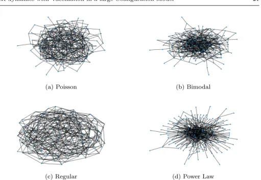
As we stated in Section 3.2.1, the mean field model corresponds to take a Poisson degree distribution. In [7], the authors establish that Poisson distribution is not realistic for the modeling of contacts, and propose the use of a bimodal distribution in which a proportion p of the population follows a Poisson law of mean C and the rest a delta-L distribution. If the whole population follows a delta distribution the associated graph is called regular. Other distribution were also proposed in [20, 34, 37], in particular the power law, found in several social networks [1, 27, 28, 39].
Thus, we consider four different networks of size N = 10000, associated to a correspondent generating function of the degree distributions, the four with mean degreeg0(1) = 5:
(a) Poisson: Degrees are distributed according a random variable Poisson P(λ) with parameterλ= 5, which givesg(z) =e5(z−1).
(b) Bimodal: a proportion p = 4/5 has degree P(3) and the rest follows a delta distribution with parameter 13, thus g(z) =pe3(z−1)+ (1−p)z13.
(c) Regular: all nodes has the same degree 5,g(z) =z5.
(d) Power Law: the probability that a node has degreekis given bypk= k
−αe−k/κ
Liα(e−1/κ) forkinN,α= 1.474 andκ= 100, resultingg(z) = Liα(z)(ze
−1/κ)
Liα(e−1/κ) whereLis(z) is thes−polylogarithm ofz. We consider an exponential cut-off aroundκ= 100 in order to have finite moments.
Here we can see that the structure makes a difference for the propagation or eradication of the disease through the existence of hubs that could play the role of super-spreaders, or almost disconnect the networks due to vaccination at higher rate. We summarize some network measures of the generated graphs, and show the numerical solutions of system (4) in each of them in order to compare the spread of the epidemic. We use thepythonpackagenetworkxfor the graph creation and the calculus of the coefficients [19], and we solve the system (4) using a Runge-Kutta 4.
We can see in the draw of the graph exposed in figure 1, that the Bimodal network has more nodes of high degree than a Poisson, and less than a Power Law network, according the results in [7].
For the epidemic evolution we take r = 4 andγ = 1, and in Table 1 we can see that networks (b) and (d) have a bigger basic reproduction number due to the size biased distribution and the expected excess degree.
Typical parameters of the nodes of social networks are the clustering coefficient, which indicate they tendency of a node to form a cluster, and the betweenness centrality, measuring the presence of the node in shortest paths between different
(a) Poisson (b) Bimodal
(c) Regular (d) Power Law
Fig. 1: An example of the graph when N=200.
Graph g00(1) R0
(a) Poisson 25 4
(b) Bimodal 61.5 9.84 (c) Regular 20 3.2 (d) Power-Law 80.31 12.83
Table 1: Network quantities
nodes, see [22]. Both play an important role in the propagation of a disease, the former due to potential contagion to larger groups of nodes, and the later because imply a quick connection between different parts of the network. Also, the closeness coefficient measures how far apart are the nodes, see [6].
In table 2 we show the average number for these measures after several exper-iments with networks of 104 nodes. We observe that density, related to the mean degree of the four networks, is similar. Nevertheless there are important differences between the averages of the clustering coefficients.
Graph Betweenness Density Clustering Closeness
×104 ×104 ×104
(a) Poisson 4.83 5.00 4.80 0.168
(b) Bimodal 3.77 5.06 11.46 0.18
(c) Regular 5.36 5.00 3.54 0.157
(d) Power Law 3.34 5.03 28.69 0.20
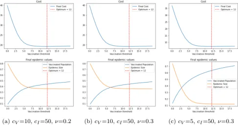
In figure 2 we present three simulations for a Bimodal graph for different op-timization costs and vaccination rates. After fixing the costs of vaccination and treatment, we look for the parameterθ∗ that realizes the minimum cost. We plot the total cost, the final number of vaccinated and the epidemic size as a function of the vaccination threshold θ, obtaining the same behavior and shape in all the studied cases.
(a)cV=10,cI=50,ν=0.2 (b)cV=10,cI=50,ν=0.3 (c)cV=5,cI=50,ν=0.3
Fig. 2: Threshold optimization for Bimodal Network
We can see from the simulation of the optimization in Figure 2 that the epi-demic size decrease notably with respect to the case without vaccination which corresponds to the vaccination threshold θ = 0. On the other hand, we observe that the epidemic size curve flatten around the valueθ∗ that minimize the cost. Therefore, it makes no sense (neither financially nor epidemiologically) to continue a vaccination program after that time, because the final cost will be bigger and the population infected will not decrease further with more vaccinated individuals.
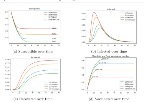
Finally we present in figure 3 the result of the simulation for the variables S,
I, RandV whenν = 0.2,cV = 10 andcI = 50, and the vaccination threshold is
the obtained by the optimization problem described above. We have thatθ∗ is 17, 12, 22 and 7 and the cost associated are 8.17, 9.89, 7.04 and 10.74 for the networks (a)-(d) respectively. Costs are higher when the epidemic is bigger since the cost of treatment is.
We expect a faster spread of the disease in the networks with a bigger clustering and closeness coefficients and lower betweenness, from the ideas exposed in the last paragraph.
Comparing Figure 3 with Tables 1 and 2 we can check that the velocity of propagation of the disease and the maximum number of infected agents is bigger in networks (b) and (d), where the basic reproduction number and the clustering and closeness coefficients are bigger and the betweenness is smaller. Moreover, the size of the epidemic in (d) is greater than the size for networks (a) and (c).
(a) Susceptible over time (b) Infected over time
(c) Recovered over time (d) Vaccinated over time
Fig. 3: Evolution of the epidemics indicators.
On the other hand, the final number of vaccinated is bigger in networks (a) and (c), almost doubling the number of vaccinated in network (d). The former are the most homogeneous in terms of degree and mixing modeling, meaning that the vaccination rate of different individuals are similar, while (d) have a big number of degree 1 individuals and a considerable proportion of high-degree nodes, whose vaccination rates have great variability.
The bimodal and power law networks seem to best reflect the interactions between people [1, 27, 28, 39]. In those cases, we observe that the spreading of the disease is faster and infect a bigger proportion of the network, due the presence of hubs, and the degree-dependent vaccination effect is not enough to contain the epidemic
Let us note that for networks (b) and (d) we have R0 ∼ 10, and the herd
immunity is reached when about 50%-60% of the population is infected or vac-cinated. In a complete network, we need about 90% of the population recovered or vaccinated. Also, for R0 ∼3−4, we need about of 70%-75% in the complete
network, while in networks (a) and (c) the vaccinated and recovered agents surpass the 90% of the population.
6 Conclusion
We considered a generalization of the SIR model on a large configuration model adding a vaccination strategy. The variables describing the dynamics were deter-mined by a Markovian contact process on a diverse population where individuals have different degrees in a network of random connectivity, the vaccination mech-anism depending on the number of possible contacts of an individual.
We derived large graph limits for the evolution of the epidemics in this context and using the probability generating functiongof the initial susceptible population we derived a system of six equation that describe the SIRV dynamics.
We then solved the associated optimal control problems, proving existence and uniqueness of the solutions under mild assumptions on cost functions. We also characterized the optimal solutions as threshold type.
For this type of strategies, we computed the impact of the vaccination process in terms of epidemic sizes, showing that the decrease of the susceptible population can be described through the generating function of the network, the proportion of IS edges and the vaccination rate, through a very simple formula.
Finally we studied four particular networks and their centrality characteristics, relating it with the epidemic indicatorR0, also depending ong. Given a maximum
vaccination rate and for fixed disease parameters, we computed the optimum vac-cination threshold and solved numerically the system of equations. We observed that in the networks that describe better the interaction of the individuals, the epidemics level of infection can be significantly different than in homogeneous models.
7 Proofs
7.1 Measures and Stochastic Differential Equations
Inspired by [10] and [15] we will represent the behavior of our dynamic as a process which is solution of a system of a stochastic differential equations derived from Poisson point measures (PPM).
We will use three different PPM for each event which modifies the quantities we are interested in: an infection, a recovery, or a vaccination. We need to identify the rates of this events and how to update the measures on the graph.
Suppose an event occur at timeT, and let us analyze the first case, an infection. For that, it is convenient first to consider
λT−(k) =rk
NTIS−
NS T−
, (20)
the rate of infection of a given k-degree individual at timeT. She will have her half-edges connected according to the quantities µT and distributed following a
multivariate hypergeometric distribution. We denote
pT−(j, l, m|k−1) = NIS T−−1 j−1 NRS T− l NV S T− m NS T−−N RS T−−N IS T−−N V S T− k−1−j−l−m NS T−−1 k−1 . (21)
Finally, givenk, j, landm, we have to update the measuresµIST ,µRST andµV ST
choosing the infected, recovered and vaccinated individuals who will be connected to the newly infected. In order to do that, we draw three vectorsu= (u1, ..., uIT−), v= (v1, ..., vRT−), andw= (w1, ..., wVT−) indicating how many links eachI,Ror
V node has with the newly infected. We considerU = S
n∈N(N0)
n and for each
µ∈ MF(N0) andn∈N we define U ⊇ U(µ, n) :=nu= (u1, ..., uhµ,1i) : hµ,1i X i=1 ui=nandui≤ζi(µ) o ,
whereζi(µ) :=Fµ−1(i) is the degree accordingµof thei-th node. In a similar way
we definev,w∈ U depending on the measuresµRST andµV ST .
Thus the number of edges of typeIS,RS orV Swill be given respectively by
ρ(u|j+ 1, µIST−) = QIT− i=1 ζi(µIST−) ui NIS T− j+1 1u∈U(µ IS T−,j+1), ρ(v|l, µRST−) = QRT− i=1 ζi(µRST−) vi NRS T− l 1u∈U(µ RS T−,l), ρ(w|m, µV ST−) = QVT− i=1 ζi(µV ST−) wi NV S T− m 1w∈U(µV ST−,m). (22) We define D(t, u, µ) = hµt,1i X i=1 δζi(µt)−ui−δζi(µt) and Df(t, u, µ) = hµt,1i X i=1 f(ζi(µt)−ui)−f(ζi(µt)).
Then, we update our measures as follows, introducing some notation:
µST =µST−−δk=µST−+∆S1(T−), µIST =µ IS T−+δk−(j+l+m+1)+D(T, u, µIS) =µIST−+∆IS1 (T−), µRST =µ RS T−+D(T, v, µRS) =µTRS−+∆RS1 (T−), µV ST =µV ST−+D(T, w, µV S) =µV ST−+∆V S1 (T−). (23)
Another event in consideration is a recovering. Here we choose uniformly an infectediand set:
µIST =µ IS T−−δζi(µIST−)=µ V S T−+∆IS2 (T−), µRST =µRST−+δζi(µIST−)=µ RS T−+∆RS2 (T−). (24)
This happens with probability 1/IT−.
The last event is vaccination. The corresponding rate isπtNtS. We remark the
strong dependence on the degree of the individual, because is more probable that a higher connectivity node to be vaccinated first. More precisely, the probability
that the new vaccinated has degree k is kµ S T−(k)
NS T−
. Once we draw the vaccinated individual, and supposing her degree isk, we update the measures as follows:
µST =µ S T−−δk=:µST−+∆S3(T−), µIST =µIST−+D(T, u, µIS) =:µIST−+∆IS3 (T−), µRST =µRST−+D(T, v, µRS) =:µRST−+∆RS3 (T−), µV ST =µV ST−+δk−(j+l+m)+D(T, w, µV S) =:µV ST−+∆V S3 (T−). (25)
Now we introduce three Poisson Point Measures that will be very useful to describe the MF(N0)-valued stochastic process (µt)t≥0. For a similar point of
view, see [10] or [15].
The first one will provide us the possible instant in which an infection occur. We define dN1(s, k, θ1, j, l, m, θ2, u, θ3, v, θ4, w, θ5) as a product measure onR+×E1
with E1 = N0×R+×(N0)3×R×(U ×R+)3, where ds and dθ are Lebesgue
measures anddnare counting measures onN0 orU, accordingly.
The degreekinfected agent will be connected withjinfected,lrecovered and
mvaccinated agents, drawn accordingu, v andw as we explained above.
We also have dN2(s, i) on E2 = R+×N a PPM with intensity γ for the recovering process. This is, for each atom we have associated a possible recovering timesand the identification numberiof the new recovered.
The last PPM, dN3(s, k, θ1, j, l, m, θ2, u, θ3, v, θ4, w, θ5) is defined inR+×E3
where E3 = E1 and it is very similar to the first one. It assign a mass to each
possible timeswhere a degreekvaccinated agent is connected with j infected,l
recovered andmvaccinated agents, drawn accordingu, v andw.
In all the cases, the auxiliary variablesθare useful to take in account the rates in this integral representation.
In order to simplify notation we will not write the dependency on the variables, and consider the following indicator functions to represent the rates:
I1=I1(s, k, θ1, j, l, m, θ2, u, θ3, v, θ4, w, θ5) =1θ1≤λs−(k)µSs−(k)1θ2≤ps−(j,l,m|k−1)1θ3≤ρ(u|j+1,µISs−) 1θ4≤ρ(v|l,µRSs−)1θ5≤ρ(w|m,µV Ss−), I2=I2(s, i) =1i≤Is−, I3=I3(s, k, θ1, j, l, m, θ2, u, θ3, v, θ4, w, θ5) =1θ1≤πs−(k)µSs−(k)1θ2≤ps−(j,l,m|k)1θ3≤ρ(u|j,µISs−) 1θ4≤ρ(v|l,µRSs−)1θ5≤ρ(w|m,µV Ss−). (26)
Now it is clear the evolution of the measures according with the events that may occur, and we are ready to write an integral form for this evolution in terms of the Poisson Point Measures, for example for the second coordinate
µISt =µ IS 0 + Z t 0 3 X k=1 Z Ek ∆ISk (s)IkdNkds. (27)
Doing the same for the four coordinates, we can write the system of Stochastic Differential Equations: µt=µ0+ Z t 0 3 X k=1 Z Ek ∆k(s)IkdNkds. (28)
Proposition 4 Given µ0 = (µS0, µIS0 , µ0RS, µV S0 ) and N1, N2, N3 there exists a
unique strong solution to the system (28) in the Skorokhod spaceD(R+,(MF(N0))4).
Proof First note that all the measures are dominated by the expectation ofµS0 +
µIS0 +µRS0 +µV S0 and the supports are bounded on the positive integers. The proof
can be completed in the same way as in [45].
7.2 Renormalization
Inspired by the techniques developed in [10] and [15] we write a renormalization of the system when the number of individuals is n and the number of edges is proportional ton. We observe that the intensity of the jump process has the same order, and deduce the scaling for the fluid limit renormalization. We prove the convergence of the solution of the finite case system of equations to the solution of (28) in the weak sense of the Skorokhod space [18].
We consider four sequences of measures indexed by n ∈ N, (µn,S), (µn,IS), (µn,RS) and (µn,V S) satisfying the system of equations (28) for eachn∈Nwith initial conditionsµn,S0 , µn,IS0 , µn,RS0 andµn,V S0 . We associate Stn, Itn, Rnt andVtn
the number of individuals in each state at timetand denoteSt,It,Rt,Vtthe sets
of the nodes susceptible, infected, recovered and vaccinated, respectively. We take the scaling µ(n),St = n1µ
S
t for each t ≤ 0 and analogously, µ(n),ISt ,
µ(n),RSt andµ(n),V St . We denoteNt(n),S =hµt(n),S, χiandSt(n)=hµ(n),St ,1iand, accordingly,Nt(n),IS,N (n),RS t ,N (n),V S t ,I (n) t ,R (n) t andV (n) t .
Finally, we scale the rates and the indicator functions associated, λnt(k) =
rkNn,ISt Nn,St , and pnt(j, l, m|k−1) = (Ntn,IS−1 j−1 )( Ntn,RS l )( Ntn,V S m )( Ntn,S−Ntn,RS−Ntn,IS−Ntn,V S k−1−j−l−m ) (Nn,S t −1 k−1 ) , I1(n)=I (n) 1 (s, k, θ1, j, l, m, θ2, u, θ3, v, θ4, w, θ5) =1θ 1≤λns−(k)nµ (n),S s− (k) 1θ2≤pns−(j,l,m|k−1)1θ3≤ρ(u|j+1,nµ (n),IS s− ) 1θ 4≤ρ(v|l,nµ (n),RS s− ) 1θ 5≤ρ(w|m,nµ (n),V S s− ) , I2(n)=I2(n)(s, i) =1i≤In s−, I3(n)=I (n) 3 (s, k, θ1, j, l, m, θ2, u, θ3, v, θ4, w, θ5) =1θ1≤πs−(k)µSs−(k)1θ2≤pns−(j,l,m|k)1θ3≤ρ(u|j,nµ (n),IS s− ) 1θ 4≤ρ(v|l,nµ (n),RS s− ) 1θ 5≤ρ(w|m,nµ (n),V S s− ) .
We assume that the sequences of initial conditions converge weakly inMF(N0)
toµS0, µIS0 , µRS0 andµV S0 when ngoes to infinity.
µ(n)t =µ (n) 0 + 1 n Z t 0 3 X k=1 Z Ek ∆(n)k (s)Ik(n)dNkds. (29) Let us define Λt= X k∈N λ(n)t (k)µ(n),St (k) X j+l+m≤k−1 pnt(j, l, m|k−1) X u∈U ρ(u|j+ 1, µ(n),ISt ) and Πt= X k∈N πtkµ(n),St (k) X j+l+m≤k pnt(j, l, m|k) X u∈U ρ(u|j, µ(n),ISt ).
Proposition 5 For allf ∈ Bb(N)and allt≥0we have the following
decomposi-tion
hµ(n),ISt , fi= X
k∈N
f(k)µ(n),IS0 (k) +A(n),IS,ft +Mt(n),IS,f,
where the finite variation is given by A(n),IS,ft = Z t 0 Λs f(k−(j+l+m+ 1)) +Df(s, u, µIS) ds − Z t 0 γhµ(n),ISs , fids+ Z t 0 ΠsDf(s, u, µIS)ds, (30)
and the associated martingale is square integrable with quadratic variation, D M(n),IS,fE t= 1 n Z t 0 Λs f(k−(j+l+m+ 1)) +Df(s, u, µIS) 2 ds + 1 n Z t 0 γhµ(n),ISs , f2ids+ 1 n Z t 0 Πs(Df(s, u, µIS))2ds.
Proof (Sketch) We first calculate the infinitesimal generator L of our process, and we write the Levy’s martingale with φ= hµ, fi andφ2. Then we apply the integration by parts formula [42], and identifying the martingales in the expression, we rearrange the terms in order to get the quadratic variation. For a detailed proof see [15].
Our fluid limit result may be proved in much the same way as proof of the main theorem of [10] but we add it for completeness.
Proof (Proof of Theorem 1)In order to prove (ii), since limε0→0tε0 =∞, is enough
to prove the result inD([0, tε0],M40,A) for ε0sufficiently small. From now on, we
take 0< ε < ε0< µIS0 , χ
.
Step 1: Tightness of the renormalization.Take (µ(n))n∈N,t∈R>0andn∈N. By assumptions, we have: hµ(n),St ,1 +χ5i+hµ (n),IS t ,1 +χ5i+hµ (n),RS t ,1 +χ5i+hµ (n),V S t ,1 +χ5i ≤ ≤ hµ(n),S0 ,1 +χ5i+hµ(n),IS0 ,1 +χ5i ≤2A (31)
This implies that the sequence µ(n)t is tight for each t. By the criterion of convergence of measure valued processes proposed by Roelly [43] we have to prove that, for each test functionf ∈ Bb(N),
hµ(n),S, fi,hµ(n),IS, fi,hµ(n),RS, fi,hµ(n),V S, fi
n∈N
is tight inD(R>0,R4). We present here the calculations only for hµ(n),IS, fibecause the others are similar or simpler. Since we have a semimartingale decomposition, applying the Rebolledo criterion for weak convergence of sequences of semimartingales, we have to prove that both the finite variation part, and the quadratic variation satisfy the Aldous criterion. We want to prove that, for allθ >0 andη >0 there existn0∈N and δ > 0 such that for all n > n0 and for all stopping times Sn andTn with
Sn< Tn< Sn+δ we have P(|A(n),IS,fT n −A (n),IS,f Sn |> η)≤θ, (32) P(|hM(n),IS,fiTn− hM (n),IS,fi Sn|> η)≤θ. (33)
For the finite variation condition (32), we take the following bound:
E h |A(n),IS,fT n −A (n),IS,f Sn | i ≤E Z Tn Sn γkfk∞hµ(n),ISs ,1ids +E Z Tn Sn X k∈N λns(k)µ (n),S s (k) X j+l+m≤k−1 pns(j, l, m|k−1)(2j+ 1)kfk∞ds +E Z Tn Sn X k∈N πsn(k)µ (n),S s (k) X j+l+m≤k pns(j, l, m|k−1)2jkfk∞ds . Since P j+l+m≤kp n
s(j, l, m|k−1)2j is twice the mean number of edges with the
infected population conditioned to having degreek, this number is bounded byk, and using the definitions ofλn,πandpwe have that:
E[|]A(n),IS,fTn −A (n),IS,f Sn | ≤ δE h γkfk∞(S0(n)+I0(n)) +rkfk∞hµ(n),S0 ,2χ2+ 3χi+νkfk∞hµ(n),S0 ,2χ2i i <∞. (34)
Then, applying Markov’s inequality:
P(|A(n),IS,fT n −A (n),IS,f Sn |> η)≤ (2γ+ 5r+ 2ν)kfk∞δA η