Giokas_unc_0153D_16279.pdf

INVESTIGATING MOLECULE-SEMICONDUCTOR INTERFACES WITH NONLINEAR SPECTROSCOPIES

Paul George Giokas

A dissertation submitted to the faculty at the University of North Carolina at Chapel Hill in partial fulfillment of the requirements for the degree of Doctor of Philosophy in the Department

of Chemistry.

Chapel Hill 2016

iii ABSTRACT

Paul George Giokas: Investigating Molecule-Semiconductor Interfaces With Nonlinear Spectroscopies

(Under the direction of Andrew M. Moran)

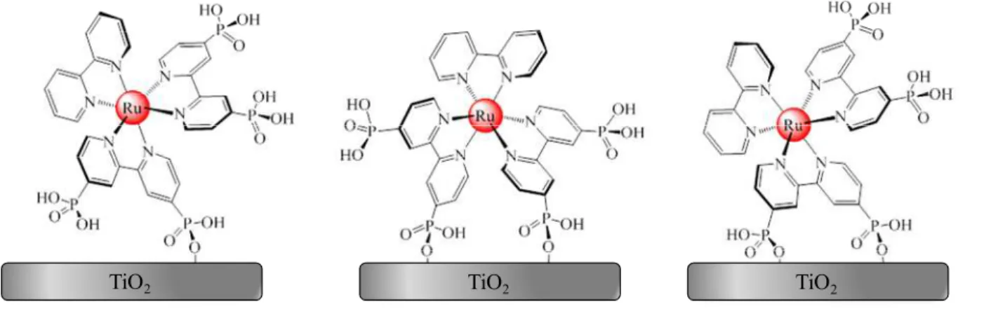
Knowledge of electronic structures and transport mechanisms at molecule-semiconductor interfaces is motivated by their ubiquity in photoelectrochemical cells. In this dissertation, optical spectroscopies are used uncover the influence of electronic coupling, coherent vibrational motion, and molecular geometry, and other factors on dynamics initiated by light absorption at such interfaces. These are explored for a family of ruthenium bipyridyl chromophores bound to TiO2, varying in the number of phosphonate anchors and the presence (or absence) of a

methylene bridge between the ligand and the TiO2. Transient absorption measurements show molecular singlet state electron injection in 100 fs or less. Resonance Raman intensity analysis suggests the electronic excitations possess very little charge transfer character. The connections drawn in this work between molecular structure and photophysical behavior contribute to the general understanding of photoelectrochemical cells.

Knowledge of binding geometry in nanocrystalline films is challenged by heterogeneity of semiconductor surfaces. Polarized resonance Raman spectroscopy is used to characterize the ruthenium chromophore family on single crystal TiO2. Chromophores display a broad

iv

phosphonate ligands, and indicates the need for careful consideration when developing surface-assembled chromophore-catalyst cells.

Electron transfer transitions occurring on the 100 fs time scale challenge conventional second-order approximations made when modeling these reactions. A fourth-order perturbative model which includes the relationship between coincident electron transfer and nuclear

relaxation processes is presented. Insights provided by the model are illustrated for a two-level donor molecule. The presented fourth-order rate formula constitutes a rigorous and intuitive framework for understanding sub-picosecond photoinduced electron transfer dynamics. Charge transfer systems fit by this model include catechol-sensitized TiO2 nanoparticles and a closely-related molecular complex, [Ti(cat)3]2-. These systems exhibit vibrational coherence coincident with back-electron transfer in the first picosecond after excitation, which suggests that

v

ACKNOWLEDGEMENTS

vi

TABLE OF CONTENTS

LIST OF TABLES ...xv

LIST OF FIGURES ... xvi

LIST OF ABBREVIATIONS AND SYMBOLS ... xxi

CHAPTER 1: INTRODUCTION ...1

1.1. A Broader Understanding of Electron Transfer at Molecule-Semiconductor Interfaces ....1

1.2.Dye-Sensitized Solar Energy Technology ...3

1.2.A. DSSC Architecture ...3

1.2.B. Artificial Photosynthesis ...5

1.3. Radiative and Non-Radiative Processes in the Photoelectrochemical Cell ...6

1.4.Understanding Interfacial Dynamics with Ultrafast Spectroscopy ...8

1.5. Structure of this Dissertation ...10

1.6 References ...12

CHAPTER 2: SPECTROSCOPY AND DYNAMICS IN CONDENSED PHASES ...17

vii

2.2. Perturbation Theory with a Density Matrix ...18

2.3. Cumulant Expansion for Fluctuations with Gaussian Statistics ...23

2.4.Third-Order Nonlinearities ...27

2.4.A. Transient Absorption Spectroscopy ...27

2.4.B. Spontaneous Raman Scattering ...30

2.4.C. Heller's Approach for Spontaneous Resonance Raman Scattering ...37

2.5 Marcus Theory ...40

2.6 Concluding Remarks ...48

2.7 References ...49

CHAPTER 3: NONLINEAR SPECTROSCOPY AND ULTRAFAST TECHNIQUES ...51

3.1. Introduction ...51

3.2.Raman Spectroscopy ...52

3.2.A. Resonance Raman Spectroscopy ...52

3.2.B. Polarized Raman Spectroscopy ...53

3.3.Pump Pulse Generation ...55

3.4.Transient Absorption Spectroscopy ...58

viii

3.4.B. Experiment Design ...58

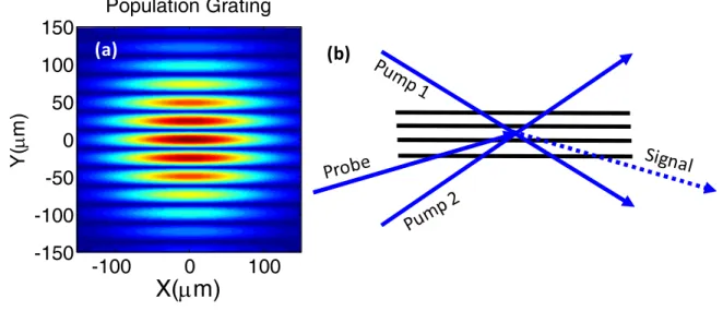
3.5.Transient Grating Spectroscopy ...61

3.5.A. Overview ...61

3.5.B. Experiment Design ...62

3.6.Conclusion ...68

3.7.References ...70

CHAPTER 4: SPECTROSCOPY AND DYNAMICS OF PHOSPHONATE- DERIVITIZED RUTHENIUM COMPLEXES ON TIO2 ...74

4.1. Introduction ...74

4.2. Background on Spectral Fitting and Physical Interpretations of Parameters ...77

4.2.A. Algorithm for Resonance Raman Intensity Analysis ...78

4.2.B. Nature of Solvent Coordinates in Ruthenium Complexes ...80

4.2.C. Correlated Line Broadening in Ruthenium Complexes ...82

4.3. Experimental Methods ...89

4.4. Results and Discussion ...94

4.4.A. Analysis of Linear Absorption Line Shapes ...94

4.4.B. Resonance Raman Measurements ...93

ix

4.5. Conclusions ...110

4.6. References ...114

CHAPTER 5: MOLECULE-SEMICONDUCTOR INTERFACIAL GEOMETRY WITH RAMAN SPECTROSCOPY...118

5.1. Introduction ...118

5.2. Background on Polarized Resonance Raman Spectroscopy ...120

5.2.A. Dipole Interaction Model ...120

5.3. Experimental Methods ...123

5.3.A. Sample Preparation ...123

5.3.B. Resonance Raman Measurements ...124

5.4. Results and Discussion ...125

5.5. Conclusions ...137

5.6. References ...138

CHAPTER 6: MODELING TIME-COINCIDENT ULTRAFAST ELECTRON TRANSFER AND SOLVATION PROCESSES AT MOLECULE-SEMICONDUCTOR INTERFACES ...140

6.1. Introduction ...140

6.2. Modeling Ultrafast Electron Transfer Kinetics...142

x

6.2.B. Fourth-Order Rate Formula ...145

6.2.C. Assumptions and Limitations of Model ...151

6.3. Second and Fourth-Order Dynamics in a Three-Level System ...152

6.4. Combining Fourth-Order Model with a First-Principles DOS for TiO2 ...157

6.4.A. Theoretical Methods ...157

6.4.B. Model Calculations ...159

6.5. Correspondence Between Second and Fourth-Order Rate Formulas ...163

6.6. Wavepacket Representation of Relaxation Processes...165

6.7. Concluding Remarks ...167

6.8. References ...169

CHAPTER 7: NONEQUILIBRIUM CHARGE TRANSFER ON SEMICONDUCTING NANOPARTICLES ...172

7.1. Introduction ...172

7.2. Background ...173

7.2.A. Modeling Catechol Back Electron Transfer ...173

7.3. Experimental Methods ...176

7.3.A. TiO2 Nanoparticle Synthesis ...176

xi

7.3.C. Transient Absorption Spectroscopy Measurements ...178

7.3.D. Transient Grating Raman Spectroscopy Measurements ...179

7.3.E. Six-Wave Mixing FSRS ...181

7.4. Results and Discussion ...184

7.4.A. Spontaneous Raman Spectroscopy ...184

7.4.B. Transient Absorption Spectroscopy ...185

7.4.C. Transient Grating Spectroscopy ...191

7.4.D. Background-Free FSRS Measurements ...194

7.5. Conclusions ...197

7.6. References ...199

CHAPTER 8: ULTRAFAST SPECTROSCOPIC SIGNATURES OF COHERENT ELECTRON TRANSFER MECHANISM IN A TRANSITION METAL COMPLEX ...204

8.1. Introduction ...204

8.2. Model for Spectroscopy and Dynamics ...207

8.2.A. Hamiltonian ...207

8.2.B. Model for Transient Absorption Signals ...209

8.2.C. Spectral Fitting of Absorbance and Resonance Raman Cross Sections ...214

xii

8.3.A. Sample Preparation ...217

8.3.B. Raman Spectroscopy ...217

8.3.C. Transient Absorption Experiments...218

8.4. Experimental Methods ...219

8.4.A. Resonance Raman Intensity Analysis and Spectral Fitting ...220

8.4.B. Decomposition of Transient Absorption Signal Components...225

8.4.C. Initiation of Vibrational Coherence by Back-Electron Transfer ...228

8.4.D. Analysis of the Back-Electron Transfer Mechanism ...231

8.5. Broader Implications for Electron Transfer Reactions ...240

8.6. Concluding Remarks ...243

8.7. References ...245

CHAPTER 9: CONCLUDING REMARKS ...249

APPENDIX A: SUPPLEMENT TO “SPECTROSCOPY AND DYNAMICS OF PHOSPHONATE- DERIVITIZED RUTHENIUM COMPLEXES ON TIO2 ...253

A.1. Spectral broadening of 400 nm laser pulses in a hollow-core fiber ...253

A.2. Sample holder for dye-sensitized TiO 2 films ...254

A.3. Solvent and pH dependence of Raman spectra ...256

xiii

A.5. Linear Absorbance Spectra ...259

A.6. Fits to Raman Excitation Profiles ...259

A.7. Fits to Linear Absorbance Spectrum ...270

A.8. Effect of Fluence on TA Line Shapes ...272

A.9. Fitting Transient Absorption Signals ...273

A.10. Raman Fit Optimization ...275

A.11. Oxidation Potentials ...277

APPENDIX B: SUPPLEMENT TO “NONEQUILIBRIUM CHARGE TRANSFER ON SEMICONDUCTING NANOPARTICLES” ...278

B.1. Linear Absorption of Sensitized Nanoparticles ...278

B.2. Resonance Raman Intensity Analysis ...279

APPENDIX C: SUPPLEMENT TO “ULTRAFAST SPECTROSCOPIC SIGNATURES OF COHERENT ELECTRON TRANSFER MECHANISMS IN A TRANSITION METAL COMPLEX” ...280

C.1. Decomposition of Transient Absorption Signals ...280

C.2. Analysis of Uncertainty in Spectral Fits ...281

C.2.A. Fits Conducted with Homogeneous Width Fixed at 2150 cm-1 ...282

C.2.B. Fits Conducted with Homogeneous Width Fixed at 3150 cm-1...285

xiv

C.4. Density Functional Theory Analysis of the Most Appropriate Basis Set ...290

C.5. Comparison of GSB, HGS, and BB Signal Components to Catechol

on TiO2 in Aqueous Solution ...291

xv

LIST OF TABLES

Table 4.1:Resonance Raman fitting parameters for all complexes in methanol ...87

Table 4.2:Resonance Raman fitting parameters for all complexes on TiO2 films ...88

Table 4.3: TA fitting Parameters for ruthenium complexes on TiO2 ...106

Table 5.1: Polarization ratios (Rx,Ry) for the chromophores on TiO2. ...129

Table 6.1: Parameters used in Model Calculations ...166

Table 7.1: Raman peak assignments. ...184

Table 7.2: Raman peak exponential fitting constants. ...194

Table 8.1. Resonance Raman Fitting Parameters ...224

Table 8.2. Organization of Quantum Numbers for Multi-Mode Basis Set. ...239

Table A.1. Complete set of Resonance Raman fitting parameters in methanol. ...257

Table A.2: Complete set of Resonance Raman fitting parameters on TiO2 films. ...258

Table A.3: Zero Crossing Fitting Parameters. ...274

Table A.4: Fitting Parameters for Figure A.22. ...274

Table B.1: Complete set of Resonance Raman fitting parameters for catechol on TiO2 ...279

Table C.1: Resonance Raman fitting for Homogeneous Width Fixed at 2150 cm-1. ...284

xvi

LIST OF FIGURES

Figure 1.1: A rudimentary DSSC consisting of a chromophore and electrode. ...4

Figure 1.2: Diagram of Interfacial Processes ...7

Figure 1.3: Example Transient Absorption Spectroscopy Signal ...9

Figure 1.4: Depiction of different binding modalities of RuP on a planar interface. ...10

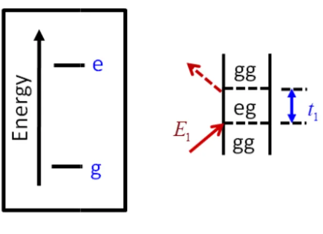
Figure 2.1- Feynman diagram for linear absorption of a two-level system ...22

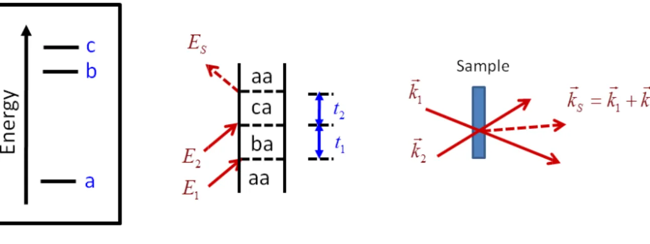
Figure 2.2: Feynman diagram for sum-frequency generation in a three-level system ...23

Figure 2.3: Feynman diagrams for a three level system ...29

Figure 2.4: Two-state example system for the investigation of spontaneous light emission ...35

Figure 2.5: Spontaneous emission Feynman diagrams ...36

Figure 2.6: Example wavepacket overlap ...38

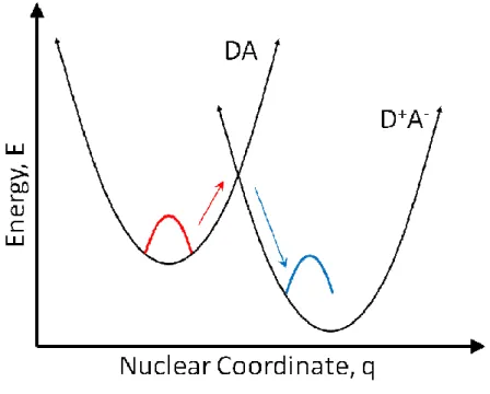
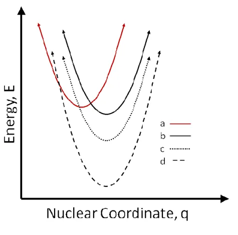
Figure 2.7: Free energy surfaces for a bimolecular donor-acceptor system ...41

Figure 2.8: Free energy regimes for a bimolecular donor-acceptor system ...45

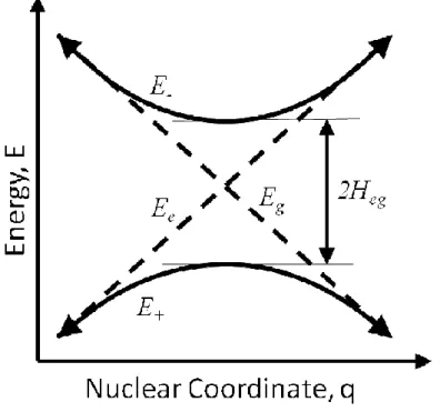
Figure 2.9: Comparison between adiabatic and nonadiabatic potential surfaces ...46

Figure 3.1: Diagram of the spontaneous Raman experimental setup ...53

Figure 3.2: Experimental Raman Polarizations ...54

Figure 3.3: Hollow Core Fiber Apparatus ...56

Figure 3.4: Hollow Core Fiber Pulse Spectra ...57

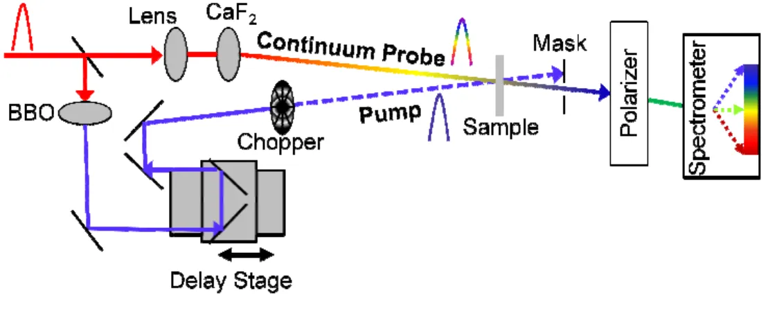
Figure 3.5: Experimental diagram for the TA measurements...59

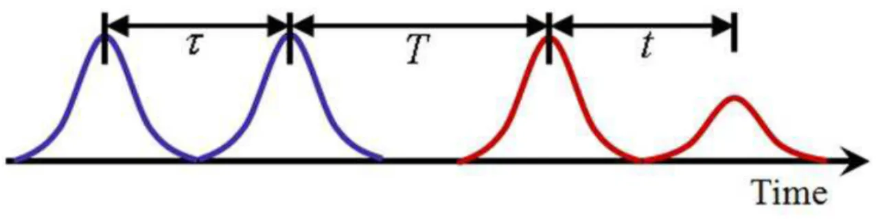
Figure 3.6: Pulse sequence in a 3rd order TG spectroscopy experiment ...62

Figure 3.7: Depiction of the Transient Grating ...63

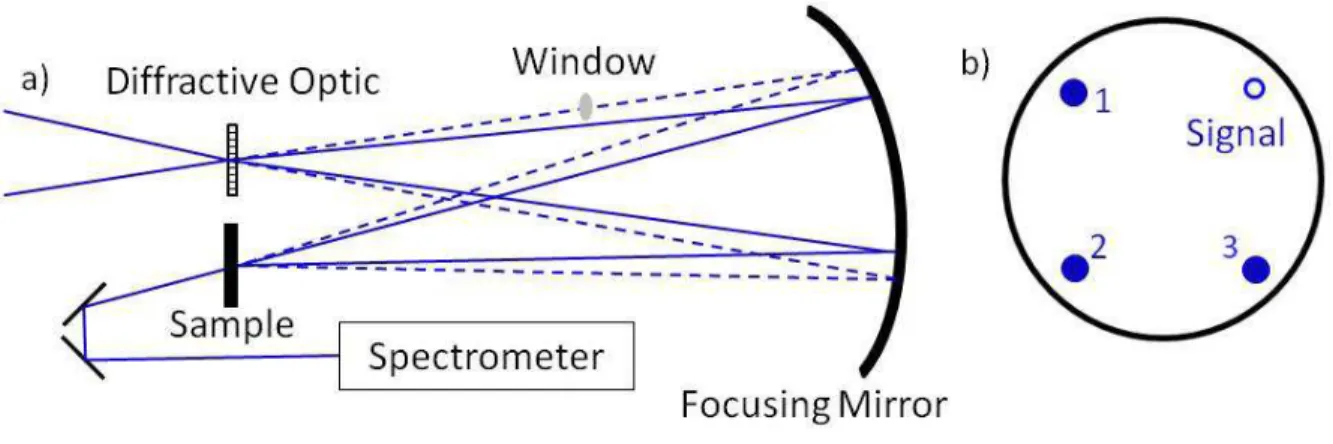
Figure 3.8: Experimental diagram for the TG Raman experiment ...64

xvii

Figure 3.10: The Sample Jet ...68

Figure 4.1: Molecular structures of phosphonated ruthenium complexes ...75

Figure 4.2: Diagram of Solvent Fluctuation Coordinates ...78

Figure 4.3: Measured absorbance spectra of all molecules ...90

Figure 4.4: Resonance Raman Spectra ...94

Figure 4.5: Fits of experimental Raman excitation profiles for 2 on TiO2 ...95

Figure 4.6: Vibrational Reorganization Energies for all molecules ...96

Figure 4.7: Potential binding motifs for Ru complexes with multiple phosphonated ligands ...97

Figure 4.8: Transient absorption spectra ...101

Figure 4.9: Normalized transient absorption signals ...103

Figure 4.10: Transient absorption time constants ...105

Figure 4.11: Zero crossing wavenumbers ...108

Figure 4.12: Relaxation scheme diagram...110

Figure 5.1: Chromophore molecular structures ...119

Figure 5.2: Dipole projection diagram ...121

Figure 5.3: Diagram of the polarized Raman experimental setup ...124

Figure 5.4: Polarized Resonance Raman spectra ...127

Figure 5.5: Average polarization ratios for RuP measured on each crystal face ...130

Figure 5.6: Average polarization ratios for RuCP measured on each crystal face ...131

Figure 5.7: Average polarization ratios for Ru2P measured on each crystal face ...132

Figure 5.8: Geometry map for RuP...133

Figure 5.9: Geometry map for RuCP ...134

xviii

Figure 5.11: Chromophore geometry distributions ...136

Figure 6.1: Wavepacket relaxation diagram ...141

Figure 6.2: Double-sided Feynman diagrams corresponding to the two rate kernels. ...146

Figure 6.3: Wavepacket calculation plots ...154

Figure 6.4: Second and fourth-order dynamics are simulated for a three-level system ...157

Figure 6.5: Conduction Band DOS of TiO2 ...158

Figure 6.6: Electron transfer dynamics computed with the first-principles DOS...161

Figure 6.7: Energy Distribution Diagram ...162

Figure 7.1: Catechol-TiO2 proposed relaxation diagram ...175

Figure 7.2: Diagram of the spontaneous Raman experimental setup ...177

Figure 7.3: Experimental diagram for the transient absorption measurements ...179

Figure 7.4: Experimental diagram for the transient grating Raman experiment ...181

Figure 7.5: Experimental diagram for the six-wave mixing FSRS experiment ...183

Figure 7.6: Resonance Raman measurement of dye- sensitized nanoparticles ...185

Figure 7.7: Transient absorption spectroscopy contour plots ...187

Figure 7.8: Transient absorption spectroscopy component contour plots ...188

Figure 7.9: Detailed fitting of the hot ground state band over the first 4 ps ...189

Figure 7.10: Raman spectra for the spontaneous and stimulated Raman experiments ...192

Figure 7.11: Stimulated Raman spectrogram from catechol-TiO2 NP solution ...193

Figure 7.12: Femtosecond Stimulated Raman peak amplitudes for the catechol loaded TiO2 ....195

Figure 7.13: FSRS spectrogram from catechol-TiO2 NP solution ...196

Figure 8.1: Four potential [Ti(cat)3]2- photoexcitation pathways. ...205

xix

Figure 8.3: The measured absorption spectrum is fit with Equation (8.19). ...220

Figure 8.4: Resonance Raman spectrum of [Ti(cat)3]2-. ...221

Figure 8.5: Experimental Raman cross sections are fit using Equation (8.20). ...223

Figure 8.6: The (a) experimental TA signal is (b) fit using Equation (8.23). ...226

Figure 8.7: The magnitude of the HGS signal component. ...228

Figure 8.8: Coherences in the TA HGS signal component. ...230

Figure 8.9: Physical picture suggested by theoretical model.. ...232

Figure 8.10: Doorway functions computed with Equation (8.20). ...234

Figure 8.11: Doorway functions computed with Equation (8.20). ...235

Figure 8.12: TA signal calculated at 500 nm with Equation (8.18) ...237

Figure 8.13: Diagram of population-to-coherence pathways ...242

Figure A.1: Hollow-core fiber setup ...253

Figure A.2: Spectra of 400 nm pulses ...254

Figure A.3: Homemade cuvette used to contain dye-sensitized films ...255

Figure A.4: Sample films are held in a homemade cuvette and oscillated ...255

Figure A.5: Raman Spectra of chromophores...256

Figure A.6: The absorption spectra of the six Ru(bpy)3 complexes ...259

Figure A.7: The excitation profile of 1 in methanol solution overlaid with fitting curve ...260

Figure A.8: The excitation profile of 1 on TiO2 overlaid with fitting curve ...260

Figure A.9: The excitation profile of 2 in methanol solution overlaid with fitting curve ...261

Figure A.10: The excitation profile of 2 on TiO2 overlaid with fitting curve ...262

Figure A.11: The excitation profile of 3 in methanol solution overlaid with fitting curve ...263

xx

Figure A.13: The excitation profile of 1C in methanol solution overlaid with fitting curve ...265

Figure A.14: The excitation profile of 1C on TiO2 overlaid with fitting curve ...266

Figure A.15: The excitation profile of 2C in methanol solution overlaid with fitting curve ...267

Figure A.16: The excitation profile of 2C on TiO2 overlaid with fitting curve ...268

Figure A.17: The excitation profile of 3C in methanol solution overlaid with fitting curve ...269

Figure A.18: The excitation profile of 3C on TiO2 overlaid with fitting curve ...270

Figure A.19: Experimental absorption spectra overlaid with model fit...271

Figure A.20: Experimental absorption spectra overlaid with model fit...272

Figure A.21: Transient absorption spectra of 1C on TiO2 ...273

Figure A.22: Normalized TA signals and fits for all ruthenium complexes in solution ...275

Figure A.23: Sum of squares error of the fit of the absorbance spectrum ...276

Figure A.24: Comparison of energy levels for each of the ruthenium complexes and TiO2 ...277

Figure B.1: Catechol-TiO2 charge transfer absorption spectrum ...278

Figure C.1: Parameters of a broadband signal component ...281

Figure C.2: Absorption spectrum fit with Equation (8.19) and the parameters in Table C.1. ...282

Figure C.3: Raman cross sections fit using Equation (8.20) and the parameters in Table C.1. ..283

Figure C.4: Absorption spectrum fit with Equation (8.19) and the parameters in Table C.2. ...286

Figure C.5: Raman cross sections fit using Equation (8.20) and the parameters in Table C.2 ...287

Figure C.6: The coherent response of the [Ti(cat)3]2- analyzed for a range of wavelengths ...289

Figure C.7: Linear absorbance spectra of [Ti(cat)3]2- and catechol on a TiO2 film. ...292

Figure C.8: TA spectrogram for the chirp-corrected signal from catechol on TiO2 ...293

xxi

LIST OF ABBREVIATIONS AND SYMBOLS

A acceptor molecule

A- reduced acceptor molecule

Å angstrom

( ) A

A

ω

α ω polarizability

α rotation angle

BBO β-barium borate BET back electron transfer

c speed of light

CB conduction band

CCD charge coupled device (1)

n

c first order coefficient of state “b” ( )

C T correlation function

cm-1 wavenumber

( ) ( ) n

χ

ω

D donor molecule

D* photoexcited dye or photoexcited donor molecule D+ oxidized dye or donor molecule

DFT density functional theory

DSPEC dye sensitized photoelectrosynthesis cell DSSC dye sensitized solar cell

xxii A

d_α

ɶ specific vibrational nuclear coordinate

∆

E(t) electric field

e- electron

e excited state index ESA excited state absorption ESE excited state emission ET electron transfer eV electron volt

∆E† energy activation barrier ε extinction coefficient

F fluence

( )

f s oscillator strength

Φ fraction of monomers photoexcited FROG frequency resolved optical gating

fs femtosecond

FSRS Femtosecond stimulated Raman spectroscopy FT Fourier Transform

FWHM full width at half maximum G

∆ free energy change

( )

G s Gaussian distribution g ground state index

( )

xxiii

(

)

G t w′ Gaussian instrument response function ( )t_n

G

GSB ground state bleach GVD group velocity dispersion

Γ damping constant

h Planck’s constant

ℏ _{reduced Planck’s constant (=h/ 2π)}

Coul

H coulombic coupling

DA

H energy gap Hamiltonian (=H_A−H_D) el ph

H − electron-phonon coupling

HOMO highest occupied molecular orbital HGS hot ground state

I Intensity or auxillary function ITO indium tin oxide

η (%) photovoltaic power conversion efficiency

DA

J dipole-dipole coupling between donor and acceptor molecules K rate function

kbt Boltzmann’s constant

k rate constant

n

k _{wavevector of pulse “n”} ( )

L ω absorption lineshape

LMCT ligand to metal charge transfer LO local oscillator

xxiv 1

−

Λ correlation time of solvent fluctuations

λ

MLCT singlet metal to ligand charge transfer 3

MLCT triplet metal to ligand charge transfer

( )

M t

solvation correlation function

µm micrometer

A

N Avogadro’s constant

ND neutral density

nm nanometer

NOPA noncollinear optical parametric amplifier OHD optical heterodyne signal detection OPA optical parametric amplifier

OPG optical parametric generation OPV organic photovoltaic

ω angular frequency

0

ω

vib

ω

( ) n

P t probability of residing in state “n” at time t. ( )

n

P kT thermal population of state “n” ( )n

P polarization of nth order

ps picosecond

xxv DA

r intermolecular distance between donor and acceptor molecules ( )

r T polarization anisotropy ˆ ( )t

ρ time dependent density operator ρ depolarization ratio

C

Q fluorescence quantum yield ( )

R t response function term

3 ( )

Ru bpy ruthenium(II)tris(bipyridine)

RuP single-ligand phosphonated Ru(bpy)3

RuCP single-ligand phosphonated Ru(bpy)3 with methylene spacers Ru2P double-ligand phosphonated Ru(bpy)3

( ) ( ) n

S t response function of nth order SNR signal-to-noise ratio

( )t

ψ wavefunction

σ cross section or Gaussian width parameter T temperature (or time interval)

τ time delay or interval

t time interval

TA transient absorption

TDPT time dependent perturbation theory TG transient grating

( ) group

t ω group velocity TOD third order dispersion

( )t

xxvi ( )

θ ω spectral phase

µ

ˆ ( )t

µ dipole operator ˆ ( )_I

V t time dependent interactive pertubation

ba

V coupling between states “a” and “b” V volume, potential, or coupling

ν frequency

A

v number of valence electrons

W rate kernel

X Beam polarization axis Y Beam polarization axis

( )t

ξ Gaussian envelope function

1

CHAPTER 1: INTRODUCTION

1.1. A Broader Understanding of Electron Transfer at Molecule-Semiconductor Interfaces

Energy is an important global resource. Population increases and industrial advancements have only increased the demand for energy in recent history. Current power requirements (as well as predicted future consumption) 1 make it necessary to develop efficient and sustainable energy conversion technologies. While several sources of renewable energy exist, most are infeasible to meet global energy demand due to excessive cost, lack of physical resources, or geographic incompatibility.2-4 Solar radiation is the most abundant power source available on the planet, delivering more energy to the Earth’s surface in one hour than was used during the entire year of 2002.5,6 The abundance of solar energy across the globe as well as the potential for cleaner, low-cost alternatives to fossil fuels has made efficient solar energy conversion an important technological goal in recent decades.5,7-23 Many approaches to harvesting solar energy have been developed, from semiconductor junction photovoltaic devices (including most

commercially available solar panels) to solar power concentrators. 8,12,13,22,24-26

2

and the molecular chromophore, where the radiation energy absorbed by the chromophore transfers to the electrode in order to be used by the cell (see Section 3). The physical and chemical properties of both the chromophore and the semiconductor influence the dynamics of electron transfer processes. As a result, wide arrays of chromophore and semiconductor pairings have been investigated in the field. 14,32,34,35

The work presented in this dissertation has thoroughly investigated the nature of electron transfer at molecule-semiconductor interfaces. Specifically, the studies presented here are concerned with uncovering the impact of molecular structure and nuclear geometry on the electron dynamics in these systems. Furthermore, the work presented here36 demonstrates that conventional second-order electron transfer models (Marcus theory)37 are insufficient to correctly model systems in which electron transfer occurs from nonequilibrium nuclear geometries and explores experimental techniques38,39 to uncover the origins of such behavior. Primarily, the work presented here:

• _{Systematically compares electron injection rates and vibrational spectra across a series of} closely related chromophores.

• _{Presents a detailed study of the binding geometry of phosphonated bipyridyl ruthenium} chromophores to TiO2 crystals with resonance Raman spectroscopy, concluding that a broad distribution of molecular orientations exists.

• _{Establishes a new fourth-order theoretical picture of the effect of nonequilibrium} processes on ultrafast electron transfer reactions in condensed phases.

3

The accomplishments presented in this dissertation all further the understanding of the molecule semiconductor interface. Such understanding is necessary for progress toward the common goal of improving the quantum efficiency of DSSC devices.

1.2. Dye-Sensitized Solar Energy Technology

1.2.A. DSSC Architecture

DSSCs utilize a light-harvesting molecule (chromophore) attached to an electrode, often a metal-oxide semiconductor. Simply, the device operates when the chromophore absorbs solar radiation, which promotes an electron into an excited state. This excited electron then transfers to the electrode, where its energy can be used to do work. 11,14,20,40 Figure 1.1a shows a basic

diagram of a DSSC.

4

Figure 1.1: (a) A rudimentary DSSC consisting of a chromophore and electrode. The chromophore molecule is attached to the semiconductor electrode such that electrons transfer from the molecule into the semiconductor, and are then drawn into the wire to their destination. (b) While still consisting of the same basic components, this DSSC utilizes nanoparticles to increase the surface area of the electrode. The orange dots represent many chromophore molecules like those in panel a. In this DSSC, the nanoparticles form a film on a conductive glass which serves the same purpose as the wire.

The light-harvesting chromophore is another main focus of improving DSSC technology. This is not surprising, as the chromophore is responsible for capturing the solar radiation and quickly and efficiently transferring it to the semiconductor, which is integral to device function. One of the largest advantages of DSSCs over bare metal-oxide nanoparticles devices is the absorption of light across the visible spectrum, rather than a relatively narrow region near the ultraviolet.18,20,32,44,45 By absorbing more of the solar spectrum, the chromophore is able to collect more energy per hour of daylight, which equates to increased power. The drastic increase

S

e

m

ic

o

n

d

u

ct

o

r

Chromophore

e

-e

-C

o

n

d

u

ct

o

r

պ

墐

5

in efficiency justifies the expense of the molecular chromophore compared to the metal-oxide electrode. Among the most popular chromophores for use in DSSCs are functionalized transition metals, particularly ruthenium-centered inorganic molecules such as, [Ru(bpy)3]2+, formally tris(bypyridine)ruthenium(II). 35,40,46-52 [Ru(bpy)3]2+ possesses a broad visible absorption band corresponding to a metal-to-ligand charge transfer (MLCT) transition which allows it to harvest a great deal of solar energy. The processes which occur between the chromophore and the semiconductor will be discussed in the next section.

1.2.B. Artificial Photosynthesis

Another key challenge undertaken by researchers designing solar cell technology in recent years is energy storage. Energy storage is a necessary concern for solar energy harvesting because any given area of the Earth’s surface does not receive constant amounts of solar

radiation, for example, at night. One solution to the problem of energy storage is the generation of solar fuels. In other words, chemical products are made using the energy collected by the solar cell which can be stored and used as chemical fuel analogous to the natural photosynthesis performed by plant life. Electrolysis of water separates it into oxygen and hydrogen gases, both of which are well-known fuels. Additionally, carbon dioxide can be converted into methane or related carbohydrates, which serve equally well as fuel.53 DSSCs which aim to generate solar fuels by such artificial photosynthetic means have been termed dye-sensitized

ր 㦀

6

This understanding includes knowledge of the physical properties (including vibrational motion and relaxation) of the chromophore and nanoparticles which impact the dynamics of these processes.

1.3. Radiative and Non-Radiative Processes in the Photoelectrochemical Cell

The work presented in this dissertation explores the ultrafast electron transfer between a semiconductor and covalently bound chromophore. TiO2 serves as the primary semiconductor surface, and in each of the following studies it is bound to one of several chromophores. The first of these chromophores is catechol. Catechol exhibits strong binding to TiO2 and sensitization is the result of the formation of a broad ligand-to-metal charge transfer (LMCT) band in the visible region. The other chromophores are all closely related to [Ru(bpy)3]2+ as discussed in the

previous section. Specifically, the ruthenium chromophores have been functionalized with phosphonic acid groups which allow covalent attachment to the semiconductor surface.34,54 This attachment is critical to the electron transfer event, as will be shown. One such ruthenium

chromophore is shown bound to TiO2 in Figure 1.2.

A number of radiative (processes involving a photon) and nonradiative processes occur at the interface of the chromophore and semiconductor.55 Light-absorption occurs when a resonant photon promotes an electron from the ruthenium metal to a bipyridine ligand, and completes within a few femtoseconds. The light-absorption causes vibrational excitation in the

7

triplet state makes ruthenium complexes attractive for increasing the quantum efficiency of electron transfer reactions.In addition, because the rate of intersystem crossing is faster than fluorescence which occurs on the µs timescale, very little of the absorbed energy is lost by radiative emission from the singlet state.

Figure 1.2: A depiction of some of the key processes which occur at the molecule-semiconductor interface. (a) Light-absorption occurs when a resonant photon promotes an electron from the ruthenium metal to a bipyridine ligand. This process occurs on the femtosecond timescale. (b) The excited electron transfers (injects) into the semiconductor surface in the 10s of femtoseconds to picoseconds after absorption. (c) The electron moves from the surface of the semiconductor into the bulk electrode. From there, it can be used by the rest of the cell to do useful work. (d) Alternatively, the electron may return to the molecule (back-electron transfer or BET) from the surface of the semiconductor. This process is not useful for harvesting solar energy.

h

ν

(b)

(d)

(a)

TiO

e

-e

-8

The excited electron transfers (injects) into the semiconductor surface in the 10s of femtoseconds to picoseconds after absorption. This process outcompetes radiative emission processes such as phosphorescence which occurs on the timescale of microseconds.50,56,57,60 After transferring to the semiconductor surface, the electron moves into the bulk states of the electrode. From there, it can be used by the rest of the cell to do useful work. If the electron becomes trappedin the states of the semiconductor,it may return to the molecule (back-electron transfer or BET). Like fluorescence and phosphorescence, BET is not a desired process for a DSPEC as the electron’s energy is lost before it can be converted to useable fuel.61,62

1.4. Understanding Interfacial Dynamics with Ultrafast Spectroscopy

The study of ultrafast processes at interfaces requires techniques which can precisely measure the dynamics in these molecule-semiconductor systems. Transient absorption

spectroscopy is a valuable technique for determining the kinetics of electron transfer reactions 63-69

ⅰю

9

Figure 1.3: Transient absorption spectroscopy signals provide information about the dynamics of short-lived species. (a) Transient absorption spectra of catechol on TiO2 nanoparticles at several delay times show a large negative feature which decays (blue arrow) while another feature grows in before decaying as well (red arrow). The negative feature corresponds to the BET process, while the positive feature reveals nuclear relaxation in the ground state. (b) The growth and decay of the associated populations as a function of delay time provides the dynamics of both interfacial processes.

A more a complete picture of the molecular interface requires the use of several specialized experimental techniques providing complementary information. In addition to the dynamics measured with transient absorption spectroscopy, the systems investigated in this dissertation have also been characterized with Resonance Raman spectroscopy. Raman

spectroscopy measures the vibrational motion of a molecule, which provides information about nuclear geometry and structure important for modeling ultrafast processes.70-72 The binding geometry of the ruthenium chromophores to TiO2 is investigated with polarized Raman spectroscopy in Chapter 5. Figure 1.4 shows various binding geometries for the

doubly-400

500

600

-25

-20

-15

-10

-5

0

5

250 fs

700 fs

1 ps

2 ps

0

1

2

Wavelength (nm)

Delay (ps)

S

ig

n

a

l

A

re

a

∆

A

(

m

O

D

)

(a)

(b)

տ 칠

10

phosphonated ruthenium chromophore. The binding mode of the ruthenium chromophores to the TiO2 surface is not trivial. The molecule-semiconductor attachment has the potential for wide variation, which affects the dynamics of electron transfer processes. Resonance Raman spectroscopy provides structural information to gain a clearer picture of the interface. The fundamental relationships between the resonance Raman spectrum and the absorption spectrum73-75 will be used to construct Raman excitation profiles to calculate vibrational reorganization energy of the ruthenium complexes76 in Chapter 4, and provide important parameters for the electron transfer model developed in Chapter 6.36

Figure 1.4: Depiction of different binding modalities of RuP on a planar interface.

1.5. Structure of this Dissertation

This chapter has presented the ideas central to the work of this dissertation which utilizes steady-state and ultrafast spectroscopies to elucidate electron transfer processes at the molecule-semiconductor interface by determining and incorporating interfacial structure into an ultrafast electron transfer model. Chapter 2 will explore past and current models used to discuss the

11

underlying physical and chemical processes in these systems, as well as the foundations of the spectroscopic techniques used to investigate them. The technical aspects of the experiments used in the work are discussed in Chapter 3, which details ultrafast spectroscopy techniques and their application to studying nanoparticle films and solutions.

The first of the experimental studies is found in Chapter 4. Transient absorption

spectroscopy is used to measure the electron transfer timescale from the MLCT states of a series of ruthenium chromophores, demonstrating the effect of increasing distance between the

molecule and semiconductor on the electronic coupling.76 Raman spectroscopy is also used to investigate the correlation between vibrational reorganization energy and these injection times. Chapter 5 contains a subsequent study performed to answer questions raised by the investigation in Chapter 4. Specifically, the orientation of the ruthenium chromophore on a TiO2 crystal is measured using polarized Raman spectroscopy in order to determine the role heterogeneity at the surface may play in the wide range of electron transfer timescales observed.

In Chapter 6, a theoretical model36 is introduced in order to describe electron injection events which occur before the chromophore has relaxed to its equilibrium geometry, which is outside the realm of the conventional Marcus theory of electron transfer. Such a model is

important especially for systems which exhibit the ultrafast electron transfer dynamics desired in a DSPEC. Illustrating the need for such a model, Chapter 7 contains a study of catechol

ⅰΉ

12

1.6. REFERENCES

(1) Hostick, D.; Belzer, D. B.; Hadley, S. W.; Markel, T.; Marnay, C.; Kinter-Meyer, M. “End-Use Electricity Demand,” NREL, 2012.

(2) Bragg-Sitton, S. M.; Boardman, R.; Zinaman, O.; Ruth, M.; Forsberg, C. “Rethinking the Future Grid: Integrated Nuclear Renewable Energy Systems,” NREL, 2014.

(3) Ladanai, S.; Vinterback, J. “Global Potential of Sustainable Biomass for Energy,” Swedish University of Agricultural Sciences, 2009.

(4) Zayas, J.; Derby, M.; Gilman, P.; Anathan, S.; Cotrell, J.; Lantz, E.; Beck, F.; Tusing, R. “Enabling Wind Power Nationwide,” U.S. Department of Energy, 2015.

(5) Morton, O. Nature 2006, 443, 19.

(6) Moore, G. F.; Brudvig, G. W. Annu. Rev. Condes. Matter Phys. 2011, 2, 303. (7) Chen, H.-Y.; Hou, J.; Zhang, S.; Liang, Y.; Yang, G.; Yang, Y.; Yu, L.; Wu, Y.; Li, G. Nat Photon 2009, 3, 649.

(8) Clarke, T. M.; Durrant, J. R. Chem. Rev. 2010, 110, 6736.

(9) Dennler, G.; Scharber, M. C.; Brabec, C. J. Adv. Mater. 2009, 21, 1323. (10) Fujishima, A.; Honda, K. Nature 1972, 238, 37.

(11) Grätzel, M. Nature 2001, 414, 338. (12) Green, M. A. Sol. Energy 2004, 76, 3.

(13) Green, M. A.; Emery, K.; Hishikawa, Y.; Warta, W.; Dunlop, E. D. Prog. Photo. Res. Appl. 2012, 20, 12.

(14) Hagfeldt, A.; Boschloo, G.; Sun, L.; Kloo, L.; Pettersson, H. Chem. Rev. 2010, 110, 6595.

(15) Liang, Y.; Xu, Z.; Xia, J.; Tsai, S.-T.; Wu, Y.; Li, G.; Ray, C.; Yu, L. Advanced Materials 2010, 22, E135.

(16) Liang, Y.; Yu, L. Accounts of Chemical Research 2010, DOI:10.1021/ar1000296. (17) Nelson, J. Curr. Opin. Solid State Mat. Sci. 2002, 6, 87.

ղ 퐐

13

(19) Park, S. H.; Roy, A.; Beaupre, S.; Cho, S.; Coates, N.; Moon, J. S.; Moses, D.; Leclerc, M.; Lee, K.; Heeger, A. J. Nature Photonics 2009, 3, 297.

(20) Peter, L. M. J. Phys. Chem. Lett. 2011, 2, 1861. (21) Service, R. F. Science 2011, 332, 293.

(22) Yu, J.; Zheng, Y.; Huang, J. Polymers 2014, 6, 2473.

(23) Zhou, H.; Yang, L.; Stuart, A. C.; Price, S. C.; Liu, S.; You, W. Angew. Chemie 2011, 50, 2995.

(24) NREL. Concentrating Solar Power Projects, 2012.

(25) Reiβ, W.; Karg, S.; Dyakonov, V.; Meier, M.; Schwoerer, M. Lumin. 1994, 60-61, 906.

(26) Tang, C. W. Appl. Phys. Lett. 1985, 48, 183.

(27) Alstrum-Acevedo, J. H.; Brennaman, M. K.; Meyer, T. J. Inorg. Chem 2005, 44, 6802.

(28) House, R. L.; Iha, N. Y. M.; Coppo, R. L.; Alibabaei, L.; Sherman, B. D.; Kang, P.; Brennaman, M. K.; Hoertz, P. G.; Meyer, T. J. J. Photochem. Photobiol. C: Photochem. Rev 2015, 25, 32.

(29) Concepcion, J. J.; Jurss, J. W.; Brennaman, M. K.; Hoertz, P. G.; Patrocinio, A. O. T.; Iha, N. Y. M.; Templeton, J. L.; Meyer, T. J. Acc. Chem Res. 2009, 42, 1954.

(30) Dismukes, G. C.; Brimblecombe, R.; Felton, G. A. N.; Pryadun, R. S.; Sheats, J. E.; Spiccia, L.; Swiegers, G. F. Acc. Chem Res. 2009, 38, 25.

(31) McEvoy, J.; Brudvig, G. Chem. Rev. 2006, 106, 4455.

(32) Swierk, J. R.; Mallouk, T. E. Chem. Soc. Rev. 2013, 42, 2357.

(33) Youngblood, W. J.; Lee, S.-H. A.; Maeda, K.; Mallouk, T. E. Acc. Chem Res. 2009, 42, 1966.

(34) Hanson, K.; Brennaman, M. K.; Luo, H.; Glasson, C. R. K.; Concepcion, J. J.; Song, W.; Meyer, T. J. Appl. Mater. Interfaces 2012, 4, 1462.

(35) Ardo, S.; Meyer, G. J. Chem. Soc. Rev. 2009, 38, 115.

ղ 퐐

14

(37) Marcus, R. A. J. Chem. Phys. 1965, 24, 966.

(38) Molesky, B. P.; Giokas, P. G.; Guo, Z.; Moran, A. M. J. Chem. Phys. 2014, 141. (39) Molesky, B. P.; Guo, Z.; Moran, A. M. J. Chem. Phys. 2015, 142.

(40) Grätzel, M. J. Photochem. Photobiol. C: Photochem. Rev 2003, 4, 145. (41) Desilvestro, J.; Gratzel, M. J. Am. Chem. Soc. 1985, 107, 2990.

(42) Diebold, U. Surf. Sci. Rep. 2003, 48, 53.

(43) Kung, H. H.; Jarrett, H. S.; Sleight, A. W.; Ferretti, A. J. Appl. Phys. 1977, 48, 2463.

(44) Xu, Y.; Schoonen, A. A. American Minerologist 2000, 85, 543. (45) Serpone, N. J. Phys. Chem. B 2006, 110, 24287.

(46) Alibabaei, L.; Luo, H.; House, R. L.; Hoertz, P. G.; Lopez, R.; Meyer, T. J. J. Mater. Chem. 2013, 1, 4133.

(47) Kalyanasundaram, K. Coord. Chem. Rev 1982, 46, 159.

(48) Balzani, V.; Credi, A.; Venturi, M. Coord. Chem. Rev 1998, 171. (49) Robertson, N. Angew. Chem. Int. Ed 2006, 45, 2338.

(50) Roundhill, D. M. Photochemistry and Photophysics of Metal Complexes; Plenum: New York, 1994.

(51) Thompson, D. W.; Ito, A.; Meyer, T. J. Pure Appl. Chem. 2013, 85, 1257. (52) Vleck Jr., A.; Busby, M. Coord. Chem. Rev 2006, 250.

(53) Morris, A. J.; Meyer, G. J.; Fujita, E. Acc. Chem Res. 2009, 42.

(54) Norris, M. R.; Concepcion, J. J.; Glasson, C. R.; Fang, Z.; Lapides, A. M.; Ashford, D. L.; Templeton, J. L.; Meyer, T. J. Inorg. Chem 2013, 52, 12492.

(55) Duncan, W.; Prezhdo, O. V. Annu. Rev. Phys. Chem. 2007, 58, 143.

ղ 퐐

15

(58) Lee, J.-J.; Rahman, M. M.; Sarker, S.; Nath, N. C. D.; Ahammad, A. J. S.; Lee, J. K. 2011.

(59) Mulazzani, Q. G.; Hoffman, M. Z.; Ford, W. E.; Rodgers, M. A. J. Phys. Chem. 1994, 98, 1145.

(60) Young, R. C.; Meyer, T. J.; Whitten, D. G. J. Am. Chem. Soc. 1976, 98, 286. (61) Knauf, R.; Kalanyan, B.; Parsons, G. N.; Dempsey, J. J. Phys. Chem. C 2015, 119, 28353.

(62) Wee, K.-R.; Sherman, B. D.; Brennaman, M. K.; Sheridan, M. V.; Nayak, A.; Alibabaei, L.; Meyer, T. J. J. Mater. Chem. A 2015, 4, 2969.

(63) Berera, R.; van Grondelle, R.; Kennis, J. T. Photosynth. Res. 2009, 101, 105. (64) Damrauer, N. H.; Cerullo, G.; Yeh, A.; Boussie, T. R.; Shank, C. V.; McCusker, J. K. Science 1997, 275, 54.

(65) Ghosh, H. N.; Asbury, J. B.; Lian, T. J. Phys. Chem. B 1998, 102, 6482.

(66) Henry, W.; Coates, C. G.; Brady, C.; Ronayne, K. L.; Matousek, P.; Towrie, M.; Botchway, S. W.; Parker, A. W.; Vos, J. G.; Browne, W. R.; McGarvey, J. J. J. Phys. Chem. A 2008, 4357.

(67) Iorio, Y. D.; Rodriguez, H. B.; San Roman, E.; Grela, M. A. J. Phys. Chem. C 2010, 113, 11515.

(68) Kuciauskas, D.; Monat, J. E.; Villahermosa, R.; Gray, H. B.; Lewis, N. S.; McCusker, J. K. J. Phys. Chem. B 2002, 106, 9347.

(69) Wallin, S.; Davidsson, J.; Modin, J.; Hammarstrom, L. J. Phys. Chem. A 2005, 109, 4697.

(70) Ambrosio, F.; Martsinovich, N.; Troisi, A. J. Phys. Chem. C 2012, 116, 2622. (71) Long, D. A. The Raman Effect: A Unified Treatment of the Theory of Raman Scattering by Molecules; Wiley: Chinchester, England, 2002.

(72) Mallick, P. K.; Danzer, G. D.; Strommen, D. P.; Kincaid, J. R. J. Phys. Chem. 1988, 92, 5628.

ղ 퐐

16

(75) Myers Kelley, A. J. Phys. Chem. A 1999, 103, 6891.

(76) Giokas, P. G.; Miller, S. A.; Hanson, K.; Norris, M. R.; Glasson, C. R. K.; Concepcion, J. J.; Bettis, S. E.; Meyer, T. J.; Moran, A. M. J. Phys. Chem. C 2013, 117.

17

CHAPTER 2: SPECTROSCOPY AND DYNAMICS IN CONDENSED PHASES

2.1. Introduction

Descriptions of condensed phase systems are much more complicated than their gas

phase counterparts due to the effect of thermal fluctuations inherent to the relatively dense

solvent environment. In other words, a large number of degrees of freedom make the explicit

treatment of all coordinates impractical or impossible. As a result, it is often necessary to treat

the system and surrounding solvent using reduced descriptions which leverage statistical

information about the ensemble (such as line widths) to gain insight into the mechanisms of

microscopic processes. 1-3

In the following sections, theoretical models for condensed phase systems will be

introduced in order to provide a context which will be referenced extensively in the subsequent

chapters. Specifically, Section 2.2 discusses perturbation theory from the perspective of the

density matrix. It will be shown how double-sided Feynman diagrams can be used to

communicate information about spectroscopies. In Section 2.3, cumulant expansions and line

broadening functions are utilized to describe the effect of fluctuations on spectroscopic

observables. Section 2.4 explores the topics of third-order nonlinear spectroscopies such as

transient grating and transient absorption before continuing into the nature of spontaneous light

emission. That topic is especially relevant to Raman spectroscopy, as well as the next, which is a

18

explores the Marcus picture of electron transfer in donor acceptor systems, which is fundamental

to discussion of nearly all of the work which follows.

2.2. Perturbation Theory with a Density Matrix

Nonlinear spectroscopies are most naturally described by following the dynamics in the

density operator instead of the wavefunction, because the time-ordering of field-matter

interactions is most transparent with this approach. This also applies to any non-radiative process

that is higher-order in the sense that the coupling between initial and final states exceeds the

regime in which traditional second-order formulas are appropriate.

The density operator is written as the outer-product in the state vector,ψ

( )

dynamics may be described with the Schrodinger equation. The equation that described the

time-evolution of the density operator is found by taking the time-derivative of the outer-product,

( )

( )

( )

_{( )}

_{( )}

( )

t t

t t t

ψ ψ ψ ψ

ψ ψ

∂ ∂ ∂

= +

∂ ∂ ∂ . (2.1)

Schrodinger's equation can be used to rewrite this formula as,

( )

( )

_{( )}

_{( )}

_{( )}

_{( )}

t t t t

t

ψ ψ

ψ ψ ψ ψ

∂ _{−   }

=_{ } + _{ }

∂  ℏ   ℏ  , (2.2)

or as

[

]

i H

t

ρ

ρ

= ∂

19

using the definition of the commutator and denoting the density operator as ρ . Equation (2.3) is

known as the quantum Liouville equation.

We next consider a situation in which a weak external perturbation interacts with the

system (e.g., external electric field). The Hamiltonian is partitioned as

( )

(0)

H =H +

λ

where ( 0 )

H is the zeroeth-order Hamiltonian and H t′

( )

convenience, we write the density operator in a basis set, where it becomes a matrix,

( )

( )

( )

mk t m t t k

ρ = ψ ψ . (2.5)

The density matrix is also expanded is orders of the perturbation,

( )

( )

( )

( )

mk t mk t mk t mk t

ρ

ρ

λρ

λ ρ

where the order of the density matrix represents the number of times that the system has

interacted with the perturbation. Substitution of Equations (2.4) and (2.6) into the quantum

Liouville equation yields

( )

(

)

(

)

(

)

( ) ( 1)

0

, exp

N N

mk N N mk N N

i

t m H t t t t k i t dt

ρ ρ ω

∞

−

′

 

= −

_∫

ℏ (2.7)

Here, N is the order of the perturbation and t_N represents the time-interval between interactions

N and N-1. Notably, Equation (2.7) contains N nested commutators (only the highest order

20

the Nth-order density operator is in hand. For example, the lowest three orders of the polarization

induced by light are given by

( )

( )

( )

( )

( )

( )

µρ

µρ

µρ

The same approach is taken without regard to the order of the polarization. In contrast, the same

orders of the polarization are written using the wavefunction as

( )

( )

( )

( )

( )

( )

( )

( )

( )

( )

( )

( )

( )

( )

( )

( )

( )

( )

( )

( )

( )

(1) (1) (0) (0) (1)

(2) (2) (0) (1) (1) (0) (2)

(3) (3) (0) (2) (1) (1) (2) (0) (3)

P t t t t t

P t t t t t t t

P t t t t t t t t t

ψ

µ ψ

ψ

µ ψ

ψ

µ ψ

ψ

µ ψ

ψ

µ ψ

ψ

µ ψ

ψ

µ ψ

ψ

µ ψ

ψ

µ ψ

= +

= + +

= + + +

. (2.9)

The simplicity of Equation (2.8) motivates use of the density operator approach instead of the

wavefunction when describing nonlinear spectroscopic techniques.

There will always be N classes of terms in

ρ

( )

of states in the system. Fortunately, it is necessary to consider only a small fraction of dominant

terms. Negligible terms correspond to off-resonant conditions in a nonlinear spectroscopy. These

dominant terms are identified using double-side Feynman diagrams. The following set of rules

can be used to quickly write the relevant terms in a nonlinear spectroscopy:

1) The density matrix must begin and end in a population (i.e., a diagonal element).

2) N+1 transition dipole matrix elements must be written. N interactions occurs with the

21

3) A propagation function must be written for each of the N intervals between field matter

interactions (these are damped waves). For example, the simplest propagation function is

written as I_eg

( )

θ

( )

ω

θ

( )

function the enforces causality,

ω

between levels g and e, and Γ_eg is damping caused by interaction with an environment.

4) Incoming arrows change the state index such that the energy of the state increases.

5) Outgoing arrows change the state index such that the energy of the state decreases (the

last interaction is ALWAYS written outgoing on the left in this thesis).

6) Arrow pointing to right (left) correspond to positive (negative) wavevectors.

7) The sum of the incident wavevectors with appropriate signs yields the wavevector of the

signal field.

8) The sign of the term is positive (negative) if we have an even (odd) number of

interactions with the bra (i.e. on the right).

We next consider two examples in which the above rules are applied. First, linear

absorption by a two-level system with ground state (g) and excited state (e). The Feynman

Figure 2.1:Feynman diagram for linear absorption of a two

generally treated as a classical field governed by an envelope function,

[

( , ) ( ) exp ( ) .

n n n n

E r t =

ξ

ω

dealing with Feynman diagrams).

Application of the rules yields the following response function:

(

R t t i t t

The Lorentzian line shape is found by Fourier transformation,

( )

0

R t i t dt

∞

∫

where the real and imaginary parts represent dispersion and absorption.

example of second-harmonic generation. Again, the rules are applied to produce the response

function, R t t

(

)

µ µ µ

ω

ω

22

Feynman diagram for linear absorption of a two-level system. The electric field

generally treated as a classical field governed by an envelope function,

]

( , ) ( ) exp ( ) .

E r t = t i k r− t +c c where k_n is the wavevector of field n (see rules 6 and 7 for

the following response function:

)

( )

1 eg 1 exp( eg1 eg1)

R t = µ θ t −iω t − Γ t .

line shape is found by Fourier transformation,

)

(

)

(

)

(

)

2

1 exp 1 1 2 ₂

eg eg eg

eg eg

i R t i t dt

ω

µ

ω ω

ω ω

− + Γ ,

where the real and imaginary parts represent dispersion and absorption. Figure 2.

harmonic generation. Again, the rules are applied to produce the response

(

)

(

)

1, 2 ba cb acexp ba1 ba1 exp ca 2 ca 2

R t t =

µ µ µ

ω

ω

The electric field E₁ is

is the wavevector of field n (see rules 6 and 7 for

(2.10)

(2.11)

2.2 presents the

harmonic generation. Again, the rules are applied to produce the response

퉠ь detection of the signal in the direction,

transformation yields the hyperpolarizability,

(

(

0 0

1 1 2

R t t i t i t dt dt

ω ω ω ω ω

∞ ∞

∝

∫∫

We now see that the signal will only be

between states a and b and c and b, respectively.

frequency mixing possess alternate response functions.

Figure 2.2: Feynman diagram for sum

experimental beam geometry is shown on the right.

2.3. Cumulant Expansion for Fluctuations with Gaussian Statistics

The condensed-phase systems investigated in this thesis are far too complex

account for all degrees of freedom. Instead we pick only a handful of degrees of freedom that the

23

detection of the signal in the direction, k_s = +k₁ k₂, defines the resonance condition yperpolarizability,

(

)

(

)

)(

)

1 2 1 1 1 2 2 1 2

1 1 2

, exp

ba cb ac

ba ba ca ca

R t t i t i t dt dt

i i

ω ω ω

µ µ µ

ω ω ω ω ω

+ +

 

 

− + Γ + − + Γ

∫∫

.

We now see that the signal will only be large when fields 1 and 2 are tuned into the energy gaps

between states a and b and c and b, respectively. Other second-order processes such as difference

frequency mixing possess alternate response functions.

Feynman diagram for sum-frequency generation in a three-level system.

experimental beam geometry is shown on the right.

for Fluctuations with Gaussian Statistics

systems investigated in this thesis are far too complex

account for all degrees of freedom. Instead we pick only a handful of degrees of freedom that the defines the resonance condition.5,6 Fourier

(2.12)

and 2 are tuned into the energy gaps

order processes such as difference

level system. The

systems investigated in this thesis are far too complex to explicitly

24

spectroscopic observables are most sensitive to. The explicit degrees of freedom define the

system, whereas the remainder of the sample is relegated to a bath.1-3 In this reduced description,

fluctuation of the system's degrees of freedom is the price we pay for partitioning the

Hamiltonian. This type of problem is ordinarily handled by letting the system couple to a bath of

an extremely large number of harmonic oscillators. Variables governed by a large number of

random degrees of freedom are expected to exhibit Gaussian statistics by the central limit

theorem. It will be shown in this section how the central limit theorem greatly simplifies the

treatment of condensed phases.

Consider a matrix element in the perturbative part of the Hamiltonian for an isolated

system which does not undergo fluctuations,

( )

(

)

(

)

(

)

0 0

ˆ _exp ˆ _exp

ˆ _exp

ba ab

b H t a b iH t H iH t a

H i

ω

′ = ′ −

′

= − , (2.13)

where it is assumed that we have expanded in a basis of eigentstatates of H₀ (i.e., the most natural choice). The matrix element then is the solution to the following equation of motion,

( )

( )

ˆ ˆ

ab

d

b H t a i b H t a

dt ′ = −

ω

For a two-level system in a condensed phase, we let the frequency undergo thermal fluctuations

and rewrite the equation of motion as

( )

( )

( )

ˆ ˆ

ab

d

b H t a i t b H t a

չ

℀

25

where

ω

( )

ω

( )

ab t

δω

( )

(

)

( )

0

ˆ ˆ _{exp exp}

t

ba ab ab

b H t a′ =H′ −iω t _−i dt′δω t′ _



∫

We next turn our attention towards an ensemble average for the equilibrium system. Integration

of the stochastic part of the equation is achieved by conducting a cumulant expansion on the

integrand and evaluating the averages (this is different that a Taylor expansion of the overall

integral). The equilibrium correlation function for the perturbative part of the Hamiltonian is

given by

( )

( )

(

)

( )

( )

( )

0 0 0

1

ˆ ˆ _{0 exp exp}

2

t t t

ba ba ab ab ab ab

H′ t H′ = −iω t _−i dτ δω τ − dτ dτ δω τ δω τ + _



∫

∫ ∫

⋯ . (2.17)

The first term is zero when fluctuations are symmetric about the mean (e.g., Gaussian

fluctuations). The second term provides information about the time scales and magnitudes of

fluctuations. All higher-order terms are zero if the fluctuations have Gaussian statistics.

Practical applications of Equation (2.17) requires choosing a form for the time-correlation

function. Kubo's function is most often used for this purpose,

( )

( )

(

)

0 exp

ab t ab ab abt

δω δω = ∆ −Λ . (2.18)

Here, ∆2_ab is the variance in the fluctuation magnitude and Λ_ab is the rate at which a fluctuation relaxes to equilibrium. With this form of the correlation function, the correlation function is

չ

℀

26

( )

( )

( )

ˆ ˆ ₀ ˆ _exp

ba ba ba ab ab

H′ t H′ = H′ _−iω t−g t _, (2.19)

where

( )

(

)

ab

ab ab ab

ab

g t = ∆ _ −Λ t + Λ −t _

Λ . (2.20)

The standard deviation, ∆_ab is usually much larger than Λ_ab for electronic energy gaps in

solution. In this realistic limit, the absorption line shape of Equation (2.11) becomes Gaussian,

.

( )

( )

2

ˆ ˆ ₀ ˆ _{exp ,}

2

ab

ba ba ba ab ab ab

H′ t H′ ≈ H′ _−iω t−∆ t _ ∆ >> Λ

  . (2.21)

Equation (2.21) can be used to obtain traditional rate formulas for electron and energy transfer in

addition to absorption and fluorescence line shapes. These formulas differ in the definition of the

perturbative part of the Hamiltonian.

Let's now reconsider absorption of the two-level system in Figure 2.1 when the levels are

coupled to a harmonic bath. For radiative processes, the perturbative part of the Hamiltonian is

given by H′ = − ⋅

µ

( )

(

)

(

)

2

2 2

1 1 1

0 2 2 2 2 exp exp 2 exp 2 2 eg

A eg eg

eg eg

eg eg

i t t i t dt

σ ω

µ

ω

ω