CONSIDERING HOLISTIC COASTAL RESPONSE TO CLIMATE-CHANGE INDUCED SHIFTS IN NATURAL PROCESSES AND ANTHROPOGENIC MODIFICATIONS
Margaret Benham Jones
A thesis submitted to the faculty at the University of North Carolina at Chapel Hill in partial fulfillment of the requirements for the degree of Masters of Science in the Department
of Geological Sciences.
Chapel Hill 2016
iii ABSTRACT
Margaret B. Jones: Considering holistic coastal response to
climate-change induced shifts in natural processes and anthropogenic modifications (Under the direction of Laura J. Moore)
Shoreline erosion can prompt the implementation of local shoreline modifications (e.g., beach nourishment, seawalls) intended to prevent erosion and protect coastal investments. These localized modifications can cause additional, potentially adverse shoreline change in neighboring locations. Here, we explore coastline response to nourishment under different climate change scenarios by coupling two existing, complimentary models of coastal processes; one addressing shoreline change related to alongshore sediment transport and the other addressing cross-shore changes in barrier island position and geometry. Results of model experiments relevant to a case study on the Virginia coast, USA, highlight the importance of regional wave climate in
iv
ACKNOWLEDGEMENTS
v
TABLE OF CONTENTS LIST OF FIGURES ... vii
LIST OF ABBREVIATIONS ... viii
CHAPTER 1 ...1
1. Introduction ...1
2. Background ...3
3. Methods ...6
3.1 Model Components ...7
3.2 Model Initialization ...9
3.3 Model Experiments ...11
3.3.1 Sea Level Rise ...11
3.3.2 Wave Climate ...11
3.3.3 Nourishment ...13
3.4 Change Analysis ...13
4. Results ...14
4.1 Effects of Climate Change Alone ...14
4.2 Effects of Stabilization ...16
vi
6. Conclusions ...24
FIGURES ...26
APPENDIX A: WAVE CLIMATE ANALYSIS ...36
APPENDIX B: ALL RESULTS ...37
vii
LIST OF FIGURES
Figure 1 – Study Site...26
Figure 2 – Schematic of Model Components ...27
Figure 3 – Flow Diagram of Model Process ...28
Figure 4 – Wave Climate Distributions ...29
Figure 5 – Relative Sea Level Rise Results ...30
Figure 6 – Wave Climate Change Results ...31
Figure 7 – Comparison between Modeled Experiments and Added Results ...32
Figure 8 – Nourishment Results for All Scenarios ...33
Figure 9 – Limited Nourishment Spreading ...34
viii
LIST OF ABBREVIATIONS BIIMS Barrier Island-Inlet Modeling System BIM Barrier Island Model
CEM Coastline Evolution Model
E East
IPCC Intergovernmental Panel on Climate Change NASA National Aeronautics and Space Administration
NE Northeast
NPS National Park Service
RRSLR Rate of Relative Sea Level Rise RSLR Relative Sea Level Rise
SCRD Shoreline Change Rate Difference TNC The Nature Conservancy
USA United States of America
USFWS United States Fish and Wildlife Service
VA Virginia
1 CHAPTER 1 1. Introduction
Barrier islands are dynamic, low-lying features occurring globally on gently sloping coastlines. In addition to their economic importance as vacation destinations and sites of commercial and residential development, barrier islands protect the mainland from storm impacts. However, as global climate continues to warm, barrier islands will be affected by climate-change induced increases in the rate of relative sea level rise (RRSLR; e.g. Mitchell et al., 2013; IPCC, 2014) and increases in the intensity of hurricanes or the frequency of the most intense hurricanes (e.g. Knutson et al., 2010; Emanuel, 2013). These effects will adversely impact development and the protective capacity of barrier island landforms (e.g., FitzGerald et al., 2008; Williams, 2013).
Barrier islands tend to respond to rising sea level by migrating upward and landward provided sufficient sand can be liberated from the shoreface and transferred to the top and back of the island via overwash, the movement of water and sediment across an island during storms or high water events (e.g., Bruun, 1962; Leatherman 1983; Cowell et al. 1995; ). If barrier islands do not receive sufficient sand from the shoreface via overwash as sea level rises, they may not maintain sufficient elevation above sea level to remain subaerial and thus drown in place or disintegrate (e.g., FitzGerald et al., 2008; Moore et al., 2010; Lorenzo-Trueba and Ashton, 2014).
2
hurricane intensity and increases in the frequency of the most intense hurricanes (Emanuel, 2013) will also alter wave climate along the U.S. East Coast. Such a shift in the recent past has been documented by Komar and Allan (2008), though not attributed to climate change. An increase in the frequency of intense hurricanes affects patterns of coastal erosion and accretion by altering the prevailing wave climate (specifically the angular distribution of wave influences), as shown by model simulations and observations of rates of coastal change (Slott et al., 2006; Moore et al., 2013; Johnson et al., 2014).
Stakeholders – organizations or individuals—who own or manage property along the coast often respond to coastal erosion by modifying the coastal zone in an attempt to “hold the line.” These efforts include beach nourishment (the addition of sand, typically from an offshore source) and shoreline armoring (the construction of physical structures such as seawalls or groins). As coastlines continue to change in response to changing climate, the tendency for humans to manipulate shoreline dynamics using these techniques will increase (Hapke et al., 2013; McNamara and Keeler, 2013). These manipulations in turn, alter both local and regional sediment budgets and nearshore processes, resulting in a strong two-way coupling between the human and natural components of the coastal system (Murray et al., 2013; Smith et al., 2015).
Although individual stakeholders and communities generally make management decisions independently of each other, previous work on multi-decadal to centurial rates of change on cuspate coastlines demonstrates that the effects of stabilization can propagate
3
fact that this approach— wherein stakeholders make management decisions independently— could have negative economic consequences for neighboring stakeholders. In these cases, adverse effects may be mitigated by undertaking a more holistic, regional approach to coastal management (Lazarus et al., 2011; Williams et al., 2013).
Here, using a case-study approach, I seek to further understanding of the way in which RSLR and changes in storm activity will alter the coupling between the natural and human
components of the coastal system on timescales relevant to human decision-making.
Specifically, I seek to understand, for this case study: (1) How the patterns and rates of shoreline change vary with different RSLR and wave climate change scenarios, (2) How strongly
stabilization efforts in one part of the system impact shoreline change rates in other parts of the system, and (3) How the effects of stabilization efforts on far-reaching parts of the coastline are altered by changes in RSLR rate and in wave climate.
In this work I focus on the Atlantic coastline of southern Maryland and Virginia, USA, and the stakeholders concerned with its management. Through discussions with local
stakeholders I identified the climate change and coastal stabilization scenarios of greatest interest to managers of these barrier islands (Accomack-Northampton Planning District Commission, 2014). Through a series of 48 model experiments using a newly-developed model of coastline change, I evaluate the likely individual and future effects of a range of RSLR, wave climate change, and mitigation scenarios on future coastline evolution.
2. Background
4
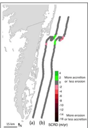
inlets (Figure 1); the most prominent of the inlets is Chincoteague Inlet, located near the northern boundary of the study area between Assateague Island and Wallops Island. Prior work has
identified this region as a hotspot of relative RSLR with modern relative RSLR rates of 3-4 mm/yr, which is 3-4 times the global average ( Sallenger et al., 2012; Mitchell et al., 2013). Since the greatest proportion of wave influence in this region is from the northeast, the prevailing direction of alongshore sediment transport is from north to south. Although these islands are in close proximity to each other, they are owned by several different organizations, each with their own management goals.
Assateague Island, the northernmost of these barrier islands, is co-owned by the National Park Service (NPS, largely in Maryland) and the United States Fish and Wildlife Service
(USFWS, in Virginia). The NPS manages Assateague Island with the goal of protecting and preserving its natural and cultural resources while allowing for public recreation on the island (National Park Service, 2002). The USFWS established the Chincoteague Wildlife Refuge in 1943 specifically to preserve habitat for migratory birds, and has since expanded their mission to include conservation of other resources as well as a commitment to providing public access for the over 1 million annual visitors who enjoy these resources (USFWS, 2015). To provide beach access in support of tourism, USFWS currently maintains a beach parking lot toward the
5
The southern terminus of Assateague Island, now known as Fishing Point or Tom’s Cove Spit, has prograded rapidly; the tip has been accreting southward at a rate of up to 55-65 m/yr since the mid-1800s (Leatherman et al., 1982; Schupp, 2013), sequestering sand delivered from the north. Fishing Point shadows nearby coastlines to the west and southwest from the effects of waves that approach from the northeast. Relatively little alongshore sediment transport occurs on the landward facing side of the spit, and the adjacent shorelines are protected from the prevailing northeasterly wave effects. Moving south along this partly sheltered shoreline, the exposure to those dominant northeasterly waves, and thus the southerly net alongshore sediment transport, increases. This gradient in net alongshore sediment transport creates an approximately 35 km “arc of erosion” south of Chincoteague Inlet (Galgano and Leatherman, 2005). As the end of Fishing Point spit extends progressively southward, the wave shadow zone also shifts southward, extending the arc of erosion. For the most part, islands within the arc of erosion have been eroding at rates of ~2-12.5 m/yr since at least the mid-1800s (Johnson et al., 2014).
Chincoteague Island, located west of southern Assateague Island, is home to ~3,000 residents of the Town of Chincoteague (U.S. Census Bureau, 2010). Due to its relatively sheltered location behind the most seaward island (Assateague Island), coastal change for Chincoteague is not addressed by this modeling work. Nevertheless, shifts in the patterns of erosion and accretion for other islands on the Virginia Eastern Shore also have the potential to affect Chincoteague
because visits to the recreational beach on Assateague Island is a critical attraction for tourists who visit the Chincoteague community (USFWS, 2015).
6
As the northern-most barrier island in the “arc of erosion” Wallops has experienced historical rates of erosion in excess of 2.5 m/yr (Johnson et al., 2014). Following stabilization efforts, including the construction of a seawall in 1992, erosion rates have decreased to near 0 m/yr (Johnson et al., 2014; NASA, 2010).
The Nature Conservancy (TNC) manages an additional 14 mixed-energy barrier islands south of Wallops Island with the goal of allowing the islands and associated habitats to evolve naturally and to conserve land and water resources. The major islands (from north to south) include Metompkin, Cedar, Parramore, Revel, Hog, Cobb, Little Cobb, Ship Shoal, Myrtle and Smith. Because of their location in the arc of erosion, Metompkin, Cedar, and Parramore Islands have historically been highly erosional, having rates of retreat between -2 m/yr and -12.5 m/yr (Johnson et al., 2014; Leatherman et al., 1982).
3. Methods
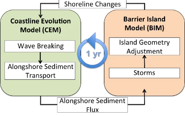
To assess the effects that climate change and human modifications may have on patterns of erosion and accretion for this region, I coupled two existing models of coastal change (first described by Ashton and Murray, 2006a, 2006b and McNamara and Werner, 2008a, 2008b). The resulting Barrier Island-Inlet Modeling System (BIIMS, Figure 3) is an exploratory coastal
change model that incorporates both alongshore and cross-shore processes. The modeling
approach focuses on key interactions that are most directly responsible for decadal coastline change (alongshore sediment transport related to coastline orientation, wave forcing, wave shadowing, and barrier migration related to RSLR and inlet dynamics). With participation from stakeholders (Accomack-Northampton Planning District Commission, 2014), I developed inputs for a suite of model experiments that allowed me to systematically test the individual and
7
shoreline change rates. To represent the key dynamics of the region and assess the effects of these components, I developed a model coastline that shares important characteristics with the physical coastline, including general shape and qualitative patterns of shoreline change.
Beginning with a simulated coastline formed from interactions and forcing the model allows me to isolate, by comparing a base case with each of the other 47 simulations, the patterns of
changes associated with all combinations of climate and stabilization scenarios. Including the base case inputs, these scenarios include a total of 4 potential RSLR rate scenarios in
combination with 3 possible wave climate distributions and 4 possible nourishment configurations (i.e. no nourishment, nourishment in the Assateague Island area only, nourishment in the Wallops Island area only, and nourishment at both sites). 3.1 Model Components
Because BIIMS is composed of two previously described and published models I provide
only the most key elements here. For more details, I refer the reader to Ashton and Murray
(2006a, 2006b) for a description of the Coastline Evolution Model (CEM), and McNamara and
Werner (2008a, 2008b) for an in-depth presentation of the Barrier Island Model (BIM).
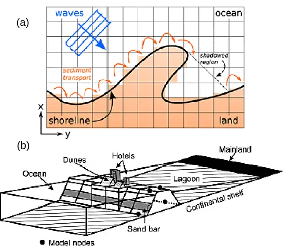
CEM is a one-contour-line model that simulates the plan-view evolution of a coastline
based on alongshore gradients in alongshore sediment flux. Each model day CEM selects a new
offshore wave approach angle from a probability density function (Figure 4), calculates wave
shoaling and refraction (over implicit locally shore-parallel shoreface contours) until waves
break in shallow depth, and then uses the CERC equation to calculate alongshore sediment flux.
Coastline curvature tends to create gradients in alongshore sediment transport, and therefore
changes in shoreline position. CEM also accounts for wave shadowing due to complex coastline
8
The primarily cross-shore model, BIM, idealizes a trapezoidal barrier island on an
unerodible slope (Figure 2b). The model is forced by historical storm data collected by Zhang et
al. who analyzed a record of U.S. Atlantic tide gauges spanning from the early 1900s to the end
of the twentieth century and identified storm events (2000). During each model year, BIM draws
a selection of storms based on these normal distributions of storm frequency, magnitude, and
duration at the Hampton Roads, VA tide gauge. During model storm surge events, the water
level rises and the island position adjusts in response. In the model, the upper shoreface erodes
during storms, and eroded sediment moves to the sandbar reservoir, and to the top and back of
the barrier. Between storms, the upper shoreface accretes. Inlets form in the model when the
elevation of the top of the barrier falls below sea level as a result of erosion. Additionally, as sea
level rises in BIM, the offshore toe of the shoreface moves up the continental slope, increasing
the slope of the upper shore face of the barrier island and simulating barrier adjustment to RSLR
(Stive and de Vriend, 1995).
Information passes between CEM and BIM each model year. At the beginning of each
model year, CEM calculates alongshore sediment flux based on wave approach angles. BIIMS
sums the net yearly sediment flux between each set of adjacent CEM cells, calculates the
gradient in flux for each cell, and passes that information to BIM. This yearly process replaces
the daily shoreline adjustments that CEM makes when running individually. In the coupled
BIIMS, BIM adjusts cross-shore position of the barrier island in response to alongshore sediment
transport gradients from CEM in addition to storm dynamics and RSLR. After BIM calculates
the new shoreface position, BIIMS passes that information to CEM and the model iterates yearly
9 3.2 Model Initialization
Prior to running BIIMS, I first initialize both components of the coupled model (i.e. CEM
and BIM) separately. To initialize CEM, I begin from a plan view shoreline with 500 m
resolution cells forming a blocky “arc” having approximately the same dimensions as the
observed arc of erosion on the Virginia shore. To represent the approximate location and
behavior of Chincoteague Inlet, on the north side of the block, I designate a line of cells, trending
in the regional alongshore direction, as sediment sinks. Because of its status as a federal
navigation channel, Chincoteague Inlet is usually dredged twice per year leading to the disposal
of 7,000 m3 of sediment outside of the channel area (Hardaway et al., 2015). In addition,
sediment is likely lost from the nearshore system to natural deposition in tidal channels landward
of the inlet. Given a lack of quantitative constraints on how rapidly the inlet draws sand away
from the adjacent shoreline, in the model I use a simple approach: half of the sediment that enters
the sink representing this inlet is lost from the system.
In CEM I impose an erosion rate of 3 m/yr near the north end of the domain. This erosion
rate was selected because (a) it produces a spit having approximately the shape and behavior of
that observed at Fishing Point (Ashton et al., 2016) and (b) it is consistent with average recent
rates of erosion of the northern end of Assateague Island (Johnson et al., 2014). Because I expect
the alongshore-transport-maximizing coastline orientation (Ashton et al., 2001) to be achieved as
waves approach the southern end of the Delmarva peninsula, I assign a boundary flux in the
southern most cell (right-most portion of the domain) that has the same value as the maximum
flux from the remainder of the domain as calculated at each timestep. This condition represents
10
As this initial blocky configuration evolves with a WIS-derived wave climate (see section
3.3.2) for 200 model years, it achieves a shape and behavior approximately consistent with
large-scale observations of plan-view shoreline change along the Delmarva Peninsula. Specifically, (a)
the northern block produces a spit, which, like Fishing Point, arcs slightly west and progrades
south at ~10-15 meters per year (as estimated from recent satellite data spanning 1984-2012), (b)
the coast immediately downdrift of this spit erodes landward at approximately 2-3 m/yr
(consistent with recent observations of the Wallops Island area coastline (Johnson et al., 2014)),
and (c) the southern block “relaxes” into a plan-view curvature reminiscent of the portion of the
Virginia Barrier Islands spanning from Cedar Island to Parramore Island.
To initialize BIM I begin from a barrier height of 1.7 m and width of 700 m, and a tidal
prism of 27 x 106 m3/m (representing the typical cross-shore width of the back-barrier basin
multiplied by the elevation difference between high tide and the back-barrier sediment surface or
between high tide and low tide, whichever is smaller) and spin up the model for 500 model years
to achieve an equilibrium state (see McNamara and Werner 2008a for further detail on
parameters and values). To smooth stochastic effects from model spin up, I use the alongshore
average of important geometric characteristics such as island height, width, and position at the
end of the spin up period as the starting point for the BIM component of the coupled model
system (BIIMS). In a separate suite of runs analyzing the potential for inlet opening, I initialize
BIM with a barrier height of 1.1 m and width of 700 m and adjust the tidal prism to 5.6 x 10⁶
m3/m. For model runs investigating inlets, I initialize the model with 3 inlets (outside the domain
of interest) so that the BIM domain is starting from an inlet density and tidal prism relationship
that is more consistent with the configuration observed in this region (this alters inlet opening but
11 3.3 Model Experiments
To compare shifts in coastline change patterns arising from different climate and nourishment scenarios, I first developed a base case model run which did not include
nourishment. The base case RSLR rate, held constant in time, is an extrapolation of the currently observed linear rate of 3 mm/yr ( Sallenger et al., 2012; Mitchell et al., 2013). The wave climate
is the same WIS-derived wave climate (see section 3.3.2) used during model initialization.
3.3.1 Sea Level Rise
The three “Low,” “High,” and “Highest” experimental sea level rise cases are non-linear
scenarios created based on global data and adjusted for the study area (Mitchell et al., 2013). (An
additional “Mid” sea level rise scenario exists for this region; however discussions with
stakeholders revealed the other three to be of greater interest to local managers). The “low”
scenario is based on conservative assumptions about future greenhouse gas emissions, the B1
scenario, and accounts for RSLR due primarily to ocean warming (Parris et al., 2012). The
“high” scenario accounts for some limited ice sheet loss and is based on the upper end of
projections from semi-empirical models. The “highest” scenario is a current practical worst-case scenario that includes maximum contributions from ice sheet loss and glacial melting (Pfeffer et al., 2008). The “low,” “high,” and “highest” scenarios include 1.1, 1.7, and 2.5 meters of total RSLR over the 50-year model run, respectively.
3.3.2 Wave Climate
Previous work has shown that plan view coastline shape and evolution depend on the
angles at which waves approach the coast. Although the approach angle and height of waves
changes on a time scale of hours to days, multi-kilometer-scale patterns of shoreline change
12
centuries or longer (Lazarus et al., 2011). Taken in aggregate, this wave climate includes the
effects of storms and seasonal patterns (Ashton and Murray, 2006a, 2006b).
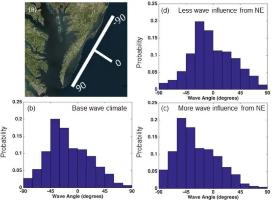
Following the approach of Johnson et al (2014) I developed the wave climate
distributions used in this study using Wave Information Systems (WIS) hindcast data from
virtual buoy 63177, located 27 km SE of the southern end of Assateague Island in a water depth
of 25 m for 1980 - 2012 (data available from http://wis.usace.army.mil/). WIS datasets provide a
variety of wave characteristics, including wave height and angle of approach, at hour-long
intervals spanning 1980-2012. I divide these data into 15o bins by wave approach angle relative
to the general coastline trend (Figure 4a). The distribution centers around -30o (waves
approaching from 30 o counterclockwise from a shore-normal direction for the average coastline
orientation—i.e. a majority of wave influence is from the E to NE) (Figure 4b), which is
consistent with observed net transport from north to south.
Given the documented effect of increasing hurricane strength on wave climate (Moore et al., 2013; Johnson et al., 2014), I address changes in storm intensity in the model by adjusting the WIS-derived wave climate used for model initialization and the base case run to reflect either a higher angle wave climate representing a greater proportion of waves approaching from the northeast (increased influence of storm-derived waves; Moore et al., 2013) or, for comparison, a lower angle wave climate representing a lesser proportion of waves approaching from the northeast (decreased influence of storm-derived waves). I accomplished this by modifying the original WIS data to create two hypothetical wave climate distributions. To create the higher
angle wave climate distribution, I rotated the angle of approach for all waves in the distribution
13
4b). The “lower angle” wave climate distribution rotates the angle of approach for all waves by
positive 15o, representing a lesser proportion of waves approaching from the NE (Figure 4c).
3.3.3 Nourishment
Based on stakeholder input (Accomack-Northampton Planning District Commission,
2014) I identified two zones within the study area (corresponding roughly to sties on Assateague
Island and Wallops Island) where nourishment activities are likely to take place in the future. I
modeled the Assateague nourishment zone as a 2 km (4 cell) stretch and the Wallops
nourishment zone as a 4 km (8 cell) stretch. At each yearly timestep, BIIMS calculates the
volume of sand lost during the previous year and adds that volume, assumed to be derived from
outside the model domain, back to the shore face to maintain the initial shoreline position for the
duration of the run.
3.4 Change Analysis
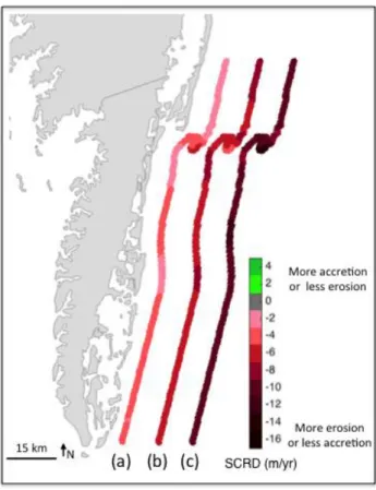
To determine shifts in patterns of coastline change associated with each climate change
scenario, I calculate the shoreline change rate difference (SCRD). The SCRD is the difference in
shoreline change rates between the 50-year base case scenario and the experimental scenario in
question, at each alongshore location. A negative SCRD indicates that the experimental scenario
results in more erosion or less accretion relative to the base case, whereas a positive SCRD
indicates that the scenario results in more accretion or less erosion relative to the base case. To
discern the effects of nourishment on coastline change, I also compare each scenario that
14
scenario, I measure island height as a function of alongshore distance at the end of each 50-year simulation experiment as a means for assessing alongshore variations in the potential for inlet opening.
4. Results
4.1 Effects of climate change alone
To determine the effects of RSLR in absence of nourishment or wave climate change, I
held the wave climate constant without nourishment and ran the model for each RSLR scenario.
For each relative sea level rise scenario (low, high, and highest) the effects of RSLR are variable alongshore: some areas are more responsive whereas others are less responsive.For all RSLR experiments, the portion of the domain representing the southern end of Assateague Island has a larger negative SCRD relative to the rest of the domain. This effect is strongest for the highest RSLR scenario (when the SCRD in the portion of the domain representing the southern end of Fishing Point is 5 m/yr more negative than the domain average). During the low RSLR scenario, the SCRD in the portion of the domain representing the southern end of Fishing Point is 3 m/yr more negative than the domain average (Figure 5). In contrast, although the portion of the domain representing Wallops Island erodes more quickly in the RSLR scenarios relative to scenarios without RSLR, it is affected less strongly by RSLR than the rest of the domain. In all three RSLR scenarios, for the portion of the domain representing Wallops Island, the SCRD is 1-2 m/yr less negative than the domain average, meaning that relatively less erosion or more accretion occurs in this area (Figure 5).
15
experiences approximately 2 m/yr more accretion or less erosion whereas a 14-cell portion of the domain representing the Wallops Island area experiences approximately 1 m/yr more erosion (Figure 6a). When the wave climate distribution is such that a lesser proportion of wave influence is from the NE (lower angle), an 11-km portion of the domain representing Wallops Island experiences up to 2 m/yr more accretion or less erosion, and an 8-km portion of the domain representing the southern end of Assateague Island experiences up to 4 m/yr more erosion or less accretion (Figure 6b).
As in the scenarios for wave climate change alone, when RSLR and wave climate change are both included, a higher wave angle distribution and lower wave angle distribution leads to less negative SCRDs for the portions of the domain representing Assateague Island and Wallops Island, respectively. Although the patterns of shoreline change in these combined runs broadly correspond to the independent effects of each scenario, the effects of RSLR and wave climate change modeled independently are not strictly additive. For the scenario in which a greater proportion of waves approaches from the NE (higher angle), the simple addition of SCRDs from the independent RSLR and wave climate change scenarios tends to under-predict the SCRD for the portion of the domain representing Assateague Island (by up to 2.5 m/yr) (Figure 7).
Similarly, in the case where a lesser proportion of waves approach from the NE (lower angle), the simple addition of shoreline change rates under-predicts the SCRD for the portion of the domain representing Wallops Island by a similar margin. The non-linear response of coastline change to sea level rise which is captured in the model explains this important difference (and is elaborated on in the Discussion section).
16
and the RSLR scenario is “high” or “highest,” there is a greater potential for inlet opening in the portion of the domain representing Wallops Island (approximate alongshore cell number 137). When a lesser proportion of wave influence is from the NE and the RSLR scenario is “high” or “highest,” there is a greater potential for inlet opening in the portion of the domain representing Assateague Island (approximate alongshore cell numbers 101-104). Neither RSLR nor wave climate change independently are associated with enhanced inlet opening in either of these areas, suggesting that the higher rate of erosion caused by the combination of climate change factors may be necessary to enhance the potential for inlet opening.
4.2 Effects of stabilization
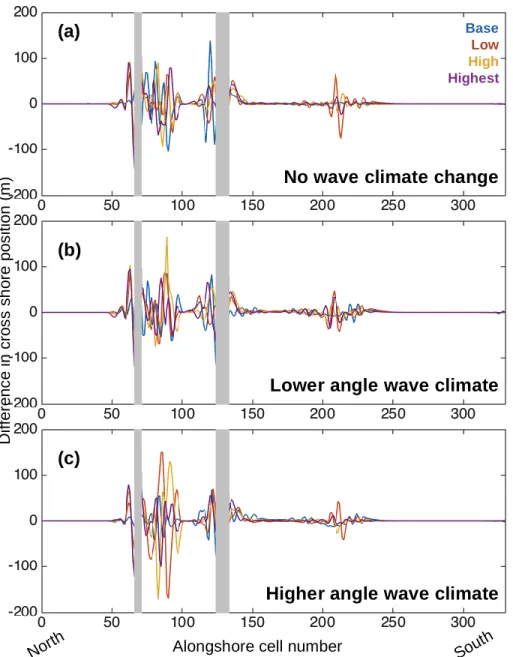
I conducted simulations in which Assateague Island and Wallops Island are nourished individually as well as scenarios in which they are nourished concurrently. However, because none of the scenarios showed appreciable effects on shoreline change rate outside the immediate vicinity of each individual nourishment zone (indicating that the effects of nourishment at each site can be evaluated individually even in experiments in which both sites are being nourished), we present only the results of simulations in which both sites were nourished simultaneously.
To discern the effects of nourishment in model runs, we compare each scenario that includes nourishment to its corresponding climate change scenario without nourishment (Figure 8). If nourishment has an effect on shoreline change outside of the nourished zones, we would expect to see altered shoreline positions immediately adjacent to the nourishment site that merge continuously into the nourished areas and into rest of the shoreline farther from the site (as in Slott et al, 2006; Ells and Murray, 2012). With limited exceptions, discussed below, such signals of alongshore-extended nourishment effects are not evident in Figure 8. In contrast, most
17
showing the differences between model runs. These undulations arise from stochastic undulations in shoreline position that occur in all scenarios (including non-nourishment scenarios) due to model discretization, as discussed in detail in the Discussion section. When calculating the difference between runs involving nourishment and the equivalent scenario without nourishment, these stochastic differences in the shoreline-position undulations appear in the shoreline position difference signal and do not represent signals of alongshore-extended nourishment effects.
I conclude, then, that in the absence of RSLR, beach nourishment seems to have almost no effect outside of the nourishment zones regardless of which of the three wave climate scenarios are used (blue lines on Figure 8 a-c). Nourishment also has no effect on the potential for inlet opening described in the previous section. For cases of low, high, or highest RSLR with no wave climate change (Figure 8a), or with a lower angle wave climate (Figure 8b), any
possible nourishment signal from the Assateague Island nourishment zone (possibly represented by altered shoreline position differences immediately to the north and south) appears limited in alongshore extent (within 2 km). In these scenarios, in the portion of the domain south of the 4-km Wallops Island nourishment zone a potential consistent alongshore effect of nourishment may be discernible up to 5 km (10 cells) from the nourishment zone. In the case of the higher angle wave climate change scenarios (Figure 8c), shoreline change patterns north of the Assateague Island nourishment zone and south of the Wallops Island nourishment zone there appears to be a 2 km additional nourishment signal on the north side of the Wallops Island nourishment zone.
18
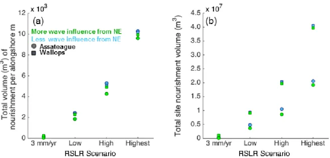
be required to maintain shoreline position. The biggest determinant of erosion rates and therefore the nourishment volumes necessary to maintain initial shoreline position is the sea level rise rate (Figure 10). In the base case RSLR, the average volume of sand needed is ~ 150 m3/m. The average volume of sand needed for the highest RSLR case is two orders of magnitude greater at ~ 10,000 m3/m. Wave climate also has a secondary effect on the erosion rates and therefore the total volume of nourishment needed. For example, for wave climates having a greater proportion of influence from the NE, the Wallops Island area needs an average of ~ 400 m3/m more
nourishment compared to Assateague Island over the course of 50 years to achieve the same steady shoreline position (a 10% difference). Given a current estimated cost of beach
nourishment of $15/m3 (USFWS, 2015), this translates to an average difference in cost for the volume of sand needed over 50 years between these two sites of ~ $6,000/m. Note that even for cases in which a lower proportion of wave influence is from the NE (favoring lower nourishment volumes per alongshore meter in the Wallops Island portion of the domain), the Wallops Island site still requires twice the total volume of nourishment needed for the Assateague Island site because the nourished length of shoreline is twice as long (Figure 10b).
5. Discussion
This modeling approach focuses on the interactions that are most directly responsible for decadal coastline change. These include alongshore sediment transport related to coastline
orientation, wave forcing, the effect of wave shadowing, and barrier migration related to RSLR
and inlet dynamics.The resulting model domain shares important characteristics with the actual
coastline, although it does not correspond in detail. The goal is to use this model to assess how patterns of coastline change may tend to shift under a range of different climate change
19
Future work with coupled cross-shore and alongshore models could build on these results by refining the representation and analysis of inlets and other barrier island processes and revising wave climate change scenarios based on current projections (for example Storlazzi et al., 2015).
I observe that the net result of adding shoreline change rates from a RSLR experiment with those from a wave climate change experiment is different from the result obtained by running a combined RSLR and wave climate change experiment (Figure 7). Specifically, the combined experiment results in higher rates of erosion than the additive case in areas of the domain whereas the wave climate change scenario alone results in more accretion relative to the base case. As sea level rises in BIIMS, the amount of shoreline retreat due to RSLR is a non-linear function of the cross-shore position, with positions farther offshore experiencing greater rates of change because the shoreface is steeper in those areas. For areas of the domain in which wave climate change results in more accretion or less erosion relative to the base case (a positive SCRD), rates of change due to RSLR are higher than they would be otherwise. This effect also explains the alongshore differences in coastline response to RSLR arising from my experiments: the Wallops Island area is more erosional than the rest of the domain, therefore it responds less strongly to RSLR relative to the rest of the domain. I also find that a high or highest RSLR rate in conjunction with higher angle wave climate leads to an increased tendency for inlets to open in the Wallops zone; however current management actions at Wallops Island (including a rock seawall and nourishment plan) are unlikely to permit inlet formation.
20
conjunction with the regional wave climate produces small undulations with stochastic positions. When the CEM model timestep is one day, these perturbations tend to be smoothed; however the yearly model timestep used in BIIMS amplifies these perturbations. This observation motivates future work on decreasing the timescale of the coupling (from yearly to daily).
In the model, I assume that beach nourishment continues over 50 years at rates sufficient to maintain a fixed shoreline position without regard for the cost of nourishment. However, my results show that the estimated total volume of sand required for nourishment will vary widely depending on the climate change scenario (depending mostly on RSLR rate, with a secondary effect from wave climate change). Given a current estimated cost of beach nourishment of $15 per m3 (USFWS, 2015), model-derived estimates for the total volume and cost of nourishment across all simulations range from 1.8 m3/m or $28,000/m for the low RSLR scenario to 10 m3/m or $150,000/m for the highest RSLR scenario. This represents a total estimated cost of
21
Surprisingly, I found that the alongshore effects of beach nourishment are likely to be limited in this region. Although I observe an alongshore signal of nourishment extending up to 5 km away from the Wallops Island nourishment zone, I see a comparatively alongshore-limited signal at the Assateague Island nourishment site. Here, nourishment effects appear to be limited within 1 km of the nourishment zone. This is in contrast to previous work that found the effects of beach nourishment to be non-local with signals of change extending tens of kilometers or more from zones of nourishment (Slott et al., 2010; Ells and Murray, 2012). To understand this difference, I need to consider how relative wave approach angles influence patterns of erosion and accretion.
When waves approach from less than ~45o relative to local coastline orientations (i.e., ‘low angle’ waves; Ashton and Murray 2006b), gradients in alongshore sediment transport tend to smooth out, or diffuse, coastline undulations (e.g. Ashton and Murray, 2006a, b).
22
transport gradients tend to smooth this subtle coastline bump, which causes the effects of the nourishment to spread alongshore (Slott et al., 2010; Ells and Murray, 2012).
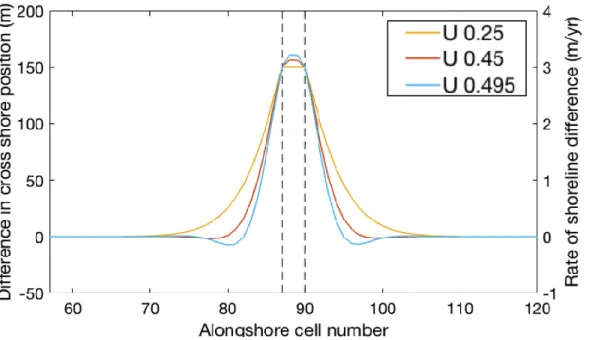
In contrast, within this study area, local wave climates are atypical. The distributions of wave influence relative to the general coastline trend (Figure 4) are such that most of the wave influence is from relative approach angles close to 45o. Waves approaching from approximately 45 o do not produce either a smoothing or roughening effect on coastline shape (e.g. Ashton and Murray, 2006a, b). In addition, given the unimodal wave climate centered on ~ 45 o relative to the coastline orientation, the influence on alongshore sediment transport from high-angle and low-angle waves is approximately equal (Figure 4). Therefore, net wave influence along most of the coastline is approximately balanced between diffusive and anti-diffusive wave influences (i.e., the coast has near zero net diffusivity). The finding that the nourishment signal does not spread alongshore is consistent with the balance between diffusive and anti-diffusive wave approach angles specific to this study area. Model experiments using CEM alone (Figure 9), show that nourishment tends to have more limited alongshore effects when the wave climate is closer to no net diffusivity. It is important to note that although shoreline stabilization through beach nourishment does not affect adjacent parts of the coastline in this study, stabilization through the use of hard structures would have an affect on downdrift portions of the coastline, regardless of the net diffusivity of the local wave climate.
23
diffusivity of the wave climate is especially close to 0 for this portion of the domain, where the mean of the wave-climate distribution falls even closer to ~ 45 o relative to local coastline orientations mean t than it does for the regional average coastline orientation. In addition, using annual time steps instead of daily time steps in CEM, in combination with the ~ 0 net diffusivity in this region, gives rise to model artifacts. When the CEM model time step is one day, subtle shoreline-shape perturbations with relatively small alongshore length scales tend to be smoothed out by the low-angle waves in the wave climate. Such smoothing occurs even if the low-angle wave influence is approximately balanced by high-angle wave influences. However, with the yearly model timestep used in BIIMS, only annual net sediment fluxes are passed from CEM to BIM, and the smoothing effects of the low-angle can be lost when the net diffusivity is ~ 0. Thus, undulations in this portion of the domain can grow. This observation motivates future work on decreasing the timescale of the coupling (from yearly to daily).
However, despite the complications in detecting alongshore-extended nourishment effect in Figure 8 that these undulations cause, we are confident in the conclusion that the alongshore extend of nourishment effects is very limited in this case-study region. Figure 10, which does not involve the complicating undulations, shows that nourishment effects tend to become more spatially localized as the net diffusivity of the wave climate decreases.
24
raising the possibility that a coordinated management strategy could be more effective than a strictly local management strategy. In such a case, the net benefits to the nourishing communities combined with those of the adjacent communities can be jointly maximized. However, where the effective diffusivity (integrated over the wave climate; Ashton and Murray 2006b) is close to 0 (the less likely of the two situations), nourishment decisions in individual communities are not coupled through the coastline smoothing mechanism, so that holistic management (in the case of nourishment only) will not likely provide additional benefits. These results suggest that
assessments of current and future regional wave climate may be important in identifying coastal areas that will benefit from a holistic approach to coastal management as climate change brings about shifts in environmental conditions that affect patterns and rates of shoreline change. 6. Conclusions
By coupling two numerical models of coastline change and exploring a range of climate scenarios (three accelerated RSLR scenarios and two wave climate change scenarios) and shoreline stabilization scenarios (two independently-controlled nourishment zones), I have developed a suite of results illustrating how multi-decadal patterns of coastline erosion and accretion could change for a region along the Mid-Atlantic Coast of the U.S. under different combinations of future conditions.
25
approaching from the NE increases erosion by 2-4 m/yr in the portion of the domain representing Wallops Island (Assateague Island) relative to the base case.
As RSLR increases, the volume of nourishment sand required to maintain the position of the shoreline increases as well (as expected). Shifts in wave climate patterns also increase or decrease the required nourishment volume in specific zones. In contrast to previous studies, in the absence of increased RSLR, nourishment has essentially no effect on coastline change rates outside of the nourished zone because the wave climate in this region has close to zero net diffusivity, which is likely to be a relatively unusual case. These results have implications for coastal management, suggesting that in this specific location and other regions having a similar wave climate, a regional, holistic approach to beach nourishment will not likely provide
26 FIGURES
27
(b)
(a)
Figure 2. (a) Schematic illustrating key components of the Coastline
28
29
Figure 4. Wave climate distributions. Negative wave angles indicate waves
30
31
Figure 6. Wave climate change scenarios. Negative shoreline change rate differences (SCRD) indicate more erosion or less accretion relative to the base case. (a) A greater proportion of waves approaching from the NE increases erosion in the portion of the domain representing Wallops Island relative to the base case (b) A lesser proportion of waves approaching from the NE
32
Figure 7. Comparison between modeled combinations of climate scenarios and addition of individual climate scenarios illustrating that in areas with higher rates of erosion relative to the rest of the domain (notably the portion of the domain representing Assateague Island for the higher angle wave climate scenario, shown in orange or the portion of the domain
33
Base
Low
High
Highest
Figure 5 Total differences in cross shore coastline position between each scenario with nourishment and without nourishment after 50 years. Grey bars are the zones where nourishment is taking place (a) Lower angle wave climate (a lesser proportion of waves approaching from the NE). (b) Higher angle wave climate (a greater proportion of wave approaching from the NE). (c) No wave climate change
No wave climate change
Lower angle wave climate
Higher angle wave climate
Alongshore cell number
North South
(a) (b) (c) D if fe re n c e i n c ro s s s h o re p o s it io n ( m )
Figure 8. Total differences in cross-shore coastline position between each climate scenario with nourishment and without nourishment after 50 years for (a) lower angle wave climate (a lesser proportion of waves approaching from the NE), (b) a higher angle wave climate (a greater proportion of wave approaching from the NE), and (c) no change in wave climate. Grey bars indicate nourishment zones. Each alongshore cell is approximately 0.5 km in length. A positive difference in cross-shore position indicates that the nourishment scenario is associated with more accretion or less erosion of the coastline relative to the same scenario without nourishment. Across all experiments nourishment produces a positive difference extending only 1-2 km from the nourishment zone. Spikes appearing between nourishment zones do not align across
34
35
36
APPENDIX A: WAVE CLIMATE ANALYSIS
I downloaded the Version 3 time series wave data from Wave Information Studies (WIS) station
63177 (depth of 25m) in November 2015. (Products are available at http://wis.usace.army.mil/). These
data are hindcasts of mean wave direction, significant wave height, period (among other attributes) at one
hour intervals from January 1980 to December 2012. WIS provides mean wave direction in degrees
clockwise from true north. To calculate the wave directions relative to the VA coast, I estimated a
coastline trend normal of ~118o based on satellite images. For each WIS data point, I calculated
37
65 REFERENCES
Accomack-Northampton Planning District Commission, 2014. Community Leader Workshop Summary Report.
Allen, M.R., Barros, V.R., Broome, J., Cramer, W., Christ, R., Church, J.A., Clarke, L., 2014. IPCC Fifth Assessment Synthesis Report-Climate Change 2014 Synthesis Report. IPCC Fifth Assess. Synth. Report-Climate Chang. 2014 Synth. Rep.
Ashton, a, Murray, a B., Arnault, O., 2001. Formation of coastline features by large-scale instabilities induced by high-angle waves. Nature 414, 296–300. doi:10.1038/35104541 Ashton, A.D., Murray, a. B., 2006a. High-angle wave instability and emergent shoreline shapes:
1. Modeling of sand waves, flying spits, and capes. J. Geophys. Res. 111, F04011. doi:10.1029/2005JF000422
Ashton, A.D., Murray, a. B., 2006b. High-angle wave instability and emergent shoreline shapes: 2. Wave climate analysis and comparisons to nature. J. Geophys. Res. F Earth Surf. 111, F04012. doi:10.1029/2005JF000423
Ashton, A.D., Nienhuis, J., Ells, K., 2016. On a neck, on a spit: Controls on the shape of free spits. Earth Surf. Dyn. 4, 193–210. doi:10.5194/esurf-4-193-2016
Bruun, P., 1962. Sea-Level Rise as a Cause of Shore Erosion, in: Proceedings of the American Society of Civil Engineers. pp. 117–130.
Cowell, P. J., Roy, P. S., & Jones, R. A. (1995). Simulation of large-scale coastal change using a
morphological behaviour model. Marine Geology,126(1), 45-61.
Ells, K., Murray, A.B., 2012. Long-term, non-local coastline responses to local shoreline stabilization. Geophys. Res. Lett. 39. doi:10.1029/2012GL052627
Emanuel, K.A., 2013. Downscaling CMIP5 climate models shows increased tropical cyclone activity over the 21st century. Proc. Natl. Acad. Sci. U. S. A. 110, 12219–24.
doi:10.1073/pnas.1301293110
FitzGerald, D.M., Fenster, M.S., Argow, B. a., Buynevich, I. V., 2008. Coastal Impacts Due to Sea-Level Rise. Annu. Rev. Earth Planet. Sci. 36, 601–647.
doi:10.1146/annurev.earth.35.031306.140139
Galgano, F.A., Leatherman, S.P., 2005. Modes and Patterns of Shoreline Change, in: Schwartz, M.L. (Ed.), Encyclopedia of Coastal Science. Springer Netherlands, Dordrecht, pp. 651– 656. doi:10.1007/1-4020-3880-1_217
Hapke, C.J., Kratzmann, M.G., Himmelstoss, E.A., 2013. Geomorphic and human influence on large-scale coastal change. Geomorphology 199, 160–170.
doi:10.1016/j.geomorph.2012.11.025
Hardaway, C.S., Milligan, D.A., Wilcox, C.A., Smith, C., 2015. Wallops Assateague Chincoteague Inlet (WACI) Geologic and Coastal Management Summary Report.
66
Recent shifts in coastline change and shoreline stabilization linked to storm climate change. doi:10.1002/esp.3650
Knutson, T.R., McBride, J.L., Chan, J., Emanuel, K., Holland, G., Landsea, C., Held, I., Kossin, J.P., Srivastava, a. K., Sugi, M., 2010. Tropical cyclones and climate change. Nat. Geosci. 3, 157–163. doi:10.1038/ngeo779
Komar, P.D., Allan, J.C., 2008. Increasing Hurricane-Generated Wave Heights along the U.S. East Coast and Their Climate Controls. J. Coast. Res. 242, 479–488. doi:10.2112/07-0894.1 Lazarus, E., Ashton, A., and Murray, A.B., 2011, Cumulative versus transient shoreline change:
Dependencies on temporal and spatial scale, J. Geophysical Research, 116, F022014, doi:10.1029/2010JF001835.
Lazarus, E.D., McNamara, D.E., Smith, M.D., Gopalakrishnan, S., Murray, A.B., 2011. Emergent behavior in a coupled economic and coastline model for beach nourishment. Nonlinear Process. Geophys. 18, 989–999. doi:10.5194/npg-18-989-2011
Leatherman, S.P., Rice, T.E., Goldsmith, V., 1982. Virginia Barrier Island Configuration : A Reappraisal. Science (80). 215, 285–287.
Leatherman, S. P. (1983). Barrier dynamics and landward migration with Holocene sea-level rise. Nature, 301, 415-417.
Lorenzo-Trueba, J., Ashton, A.D., 2014. Rollover, drowning, and discontinuous retreat: Distinct modes of barrier response to sea-level rise arising from a simple morphodynamic model. J. Geophys. Res. Earth Surf. 119, 779–801. doi:10.1002/2013JF002941
McNamara, D.E., Keeler, A., 2013. A coupled physical and economic model of the response of coastal real estate to climate risk. Nat. Clim. Chang. 3, 559–562. doi:10.1038/nclimate1826 McNamara, D.E., Murray, B.A., Smith, M.D., 2011. Coastal sustainability depends on how
economic and coastline responses to climate change affect each other. Geophys. Res. Lett. 38. doi:10.1029/2011GL047207
McNamara, D.E., Werner, B.T., 2008a. Coupled barrier island-resort model: 1. Emergent
instabilities induced by strong human-landscape interactions. J. Geophys. Res. F Earth Surf. 113, F01016. doi:10.1029/2007JF000840
McNamara, D.E., Werner, B.T., 2008b. Coupled barrier island-resort model: 2. Tests and predictions along Ocean City and Assateague Island National Seashore, Maryland. J. Geophys. Res. Earth Surf. 113. doi:10.1029/2007JF000841
Mitchell, M., Hershner, C., Julie, H., Schatt, D., Mason, P., Eggington, E., 2013. Recurrent Flooding Study for Tidewater Virginia. Virginia Inst. Mar. Sci. Cent. Coast. Resour. Manag.
Moore, L.J., List, J.H., Williams, S.J., Stolper, D., 2010. Complexities in barrier island response to sea level rise: Insights from numerical model experiments, North Carolina Outer Banks. J. Geophys. Res. doi:10.1029/2009JF001299
67
Murray, A.B., Gopalakrishnan, S., McNamara, D.E., Smith, M.D., 2013. Progress in coupling models of human and coastal landscape change. Comput. Geosci. 53, 30–38.
doi:10.1016/j.cageo.2011.10.010
NASA, 2010. Final programmic environmental impact statement Wallops Flight Facility shoreline restortion and infrastructure protection program.
National Park Service, 2002. Assateague Island National Seashore Long Range Interpretive Plan. Parris, A., Bromirski, P., Burkett, V., Cayan, D., Culver, M., Hall, J., Horton, R., Knuuti, K.,
Moss, R., Obeysekera, J., Sallenger, A., Weiss, J., 2012. Global Sea Level Rise Scenarios for the US National Climate Assessment. NOAA Tech Memo OAR CPO 1–37.
Pfeffer, W.T., Harper, J.T., O’Neel, S., 2008. Kinematic constraints on glacier contributions to 21st-century sea-level rise. Science 321, 1340–1343. doi:10.1126/science.1159099 Sallenger, A.H., Doran, K.S., Howd, P. a., 2012. Hotspot of accelerated sea-level rise on the
Atlantic coast of North America. Nat. Clim. Chang. 2, 1–5. doi:10.1038/nclimate1597 Schupp, C., 2013. Assateague Island National Seashore Geologic Resources Inventory Report. Slott, J.M., Murray, A. B., Ashton, A.D., 2010. Large-scale responses of complex-shaped
coastlines to local shoreline stabilization and climate change. J. Geophys. Res. F Earth Surf. 115, F03033. doi:10.1029/2009JF001486
Slott, J.M., Murray, A.B., Ashton, A.D., Crowley, T.J., 2006. Coastline responses to changing storm patterns. Geophys. Res. Lett. 33. doi:10.1029/2006GL027445
Smith, M.D., Murray, A.B., Gopalakrishnan, S., Keeler, A.G., Landry, C.E., McNamara, D., Moore, L.J., 2015. , Chapter 7 – Geoengineering Coastlines? From Accidental to
Intentional, in: Coastal Zones, Solutions for the 21st Century. Elsevier. doi:10.1016/B978-0-12-802748-6.00007-3
Stive, M.J.F., de Vriend, H.J., 1995. Modelling shoreface profile evolution. Mar. Geol. 126, 235–248. doi:10.1016/0025-3227(95)00080-I
Storlazzi, C.D., Shope, J.B., Erikson, L.H., Hegermiller, C.A., Barnard, P.L., 2015. Future Wave and Wind Projections for United States and United States-Affiliated Pacific Islands [WWW Document]. U.S. Geol. Surv. Open-File Rep. 2015–1001.
doi:http://dx.doi.org/10.3133/ofr20151001
U.S. Census Bureau, 2010. 2010 Profile of General Population and Housing Characteristics; Chincoteague town,Virginia. [WWW Document]. Online. URL
http://factfinder.census.gov/faces/nav/jsf/pages/community_facts.xhtml (accessed 6.3.16). USFWS, 2015. Chincoteague and Wallops Island National Wildlife Refuges: Comprehensive
Conservation Plan.
Williams, S.J., 2013. Sea-level rise implications for coastal regions. J. Coast. Res. 63, 184–196. doi:10.2112/SI63-015.1
68 Earth Surf. 118, 887–899. doi:10.1002/jgrf.20066
Woodruff, J.D., Irish, J.L., Camargo, S.J., 2013. Coastal flooding by tropical cyclones and sea-level rise. Nature 504, 44–52. doi:10.1038/nature12855
Zhang, K., Douglas, B.C., Leatherman, S.P., 2000. Twentieth-century storm activity along the U.S. East Coast. J. Clim. 13, 1748–1761.