Two Dimensional Diffusion of Colloidal Particles on Supported Lipid Bilayers

(1)

Leiden University

Soft Matter Physics

Master Project

Two Dimensional Diffusion of Colloidal

Particles on Supported Lipid Bilayers

Author:

Ernst Jan

_Vegter

Supervisors:

Casper

_{van der Wel}

Daniela

_Kraft

(2)

1 Abstract

(5)

2 Introduction and Motivation

A cellular membrane forms the boundary of all cells in nature. It consists of a lipid bilayer in which many biological molecules reside, of which transmem-brane proteins form the majority. Memtransmem-brane proteins are targeted in many infectious diseases, such as Alzheimer’s disease [22]. Since the lipid bilayer is fluid, transmembrane proteins are free to diffuse in the plane of the lipid bilayer [24]. Figure 1 shows the diffusion of lipids in the lipid bilayer.

Figure 1: A schematic picture of the cross section of a lipid bilayer. In the left picture, we label a region of lipids (black). As time passes by, these lipid diffuse freely through the lipid bilayer. This gives rise to the right picture, in which the black lipids have spread through in the lipid bilayer. From [28].

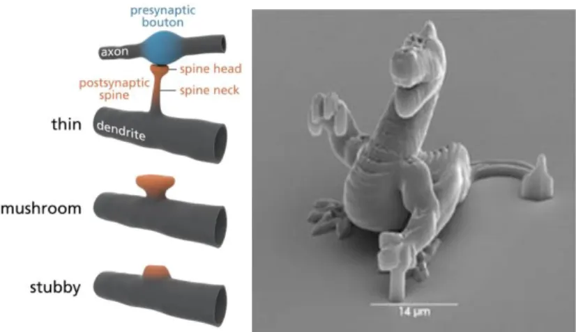
It has recently been shown in theory and simulation [17] [14] that the dif-fusion of substrate-attached proteins is strongly influenced by the geometry of the substrate. Different membrane shapes may cause local variations in the protein concentration or dynamically trap them at certain locations. As cells and their membranes are found in various geometries (figure 2), the link between geometry and diffusion is of paramount importance.

(6)

Figure 2: Left: The mushroom-like shape of the top of a dendritic spine (part of the nerve system) is an example of a special geometry in nature. From [29]. Right: Example of a tiny (µmscale) dragon that was 3D printed using two-photon polymerization. From [1].

(7)

Colloid

Lipid Bilayer (cell membrane)

Substrate with geometry modelling the biological system (e.g. synapse) -> TPA printed substrate (ORMOCER) ~1 mm

~10 mm

Linker

(8)

3 PART I: Lipid bilayers on various substrates

In this part our experiments on polymer, glass, and ORMOCER supported lipid bilayers will be described. Sample names for all samples shown can be found in table 10 (section 3.8) on page 54.

3.1 Experimental Goal I: Polymer Supported Lipid

Bi-layers

As explained in section 2, we want to create a homogeneous and fluid lipid bilayer on an ORMOCER substrate. To minimize the contribution of the substrate to the fluidity and homogeneity of the lipid bilayer, we will use the method described by K¨ugler and Knoll in 2002 [15]. The authors claim to achieve more mobile lipid bilayers by putting a polymer support (like a ‘cushion’) between the lipid bilayer and the substrate.

(9)

3.2 Methods and Materials

3.2.1 Chemicals

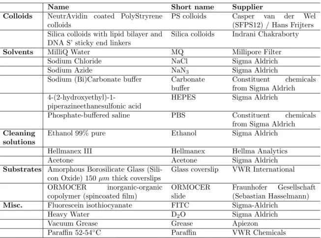
In the table below, all chemicals used in this research are listed. The table includes the chemicals used in part II of this report.

Name Short name Supplier Polymers Poly(ethylenimine) PEI Sigma-Aldrich

Poly(sodium 4-styrenesulfonate) PSS Sigma-Aldrich

Poly(allylamine hydrochloride) PAH Sigma-Aldrich

Poly(ethylene glycol) 2-aminoethyl ether biotin

PEG-Biotin Sigma-Aldrich

Lipids 1,2-dioleoyl-sn-glycero-3-phosphocholine

DOPC Avanti Polar Lipids

1,2-dioleoyl-sn-glycero-3-phospho-(1’-rac-glycerol)

DOPG Avanti Polar Lipids

1,2-dioleoyl-sn-glycero-3-

phosphoethanolamine-N-[methoxy(polyethylene

glycol)-2000]

DOPE-Peg Avanti Polar Lipids

1,2-dipalmitoyl-sn-glycero-

3-phosphoethanolamine-N-[methoxy(polyethylene

glycol)-2000]

DPPE-Peg Avanti Polar Lipids

1,2-Dioleoyl-sn-glycero-3- phosphoethanolamine-N-(lissaminerhodamine B sulfonyl)

DOPE-Rho Avanti Polar Lipids

1,2-Dioleoyl-sn-glycero-3- phosphoethanolamine-N-(7-nitro-2-1,3-benzoxadiazol-4-yl)

DOPE-NBD Avanti Polar Lipids

1-palmitoyl-2-oleoyl-sn-glycero-3- phosphocholine-N-(7-nitro-2-1,3-benzoxadiazol-4-yl)

POPC-NBD Avanti Polar Lipids

1-oleoyl-2-6-[(7-nitro-2-1,3- benzoxadiazol-4-yl)amino]hexanoyl-sn-glycero-3-phosphocholine

PC-C6-NBD Avanti Polar Lipids

1,2-Distearoyl-sn-glycero- 3-phosphoethanolamine-N-[biotinyl(polyethylene glycol)-2000] DPSE- PEG(2000)-Biotin

Avanti Polar Lipids

1,2-dioleoyl-sn-glycero-3-phosphoethanolamine-N-(cap biotinyl)

DOPE-Cap-Biotin

Avanti Polar Lipids

(10)

Name Short name Supplier Colloids NeutrAvidin coated PolyStryrene

colloids

PS colloids Casper van der Wel

(SFPS12) / Hans Frijters Silica colloids with lipid bilayer and

DNA S’ sticky end linkers

Silica colloids Indrani Chakraborty

Solvents MilliQ Water MQ Millipore Filter

Sodium Chloride NaCl Sigma Aldrich

Sodium Azide NaN3 Sigma Aldrich

Sodium (Bi)Carbonate buffer Carbonate

buffer

Constituent chemicals

from Sigma Aldrich

4-(2-hydroxyethyl)-1-piperazineethanesulfonic acid

HEPES Sigma Aldrich

Phosphate-buffered saline PBS Constituent chemicals

from Sigma Aldrich

Cleaning solutions

Ethanol 99% pure Ethanol Sigma Aldrich

Hellmanex III Hellmanex Hellma Analytics

Acetone Acetone Sigma Aldrich

Substrates Amorphous Borosilicate Glass

(Sili-con Oxide) 150µmthick coverslips

Glass coverslip VWR International

ORMOCER inorganic-organic

copolymer (spincoated film)

ORMOCER slide

Fraunhofer Gesellschaft

(Sebastian Hasselmann)

Misc. Fluorescein isothiocyanate FITC Sigma-Aldrich

Heavy Water D2O Sigma Aldrich

Vacuum Grease Grease Apiezon

Paraffin 52-54◦C Paraffin VWR Chemicals

Table 1: An overview of the chemicals used in this thesis. The short name will be used in the proceeding paragraphs.

PAH·FITC

To be able to observe the final layer of PAH on our samples, we synthesized PAH·FITC. The amine group (-NH2) on the PAH binds to the isothiocyanate (-N=C=S) group on the FITC. To establish this reaction, a pH 9.5 carbo-nate buffer was prepared. In this buffer we dissolved 2 g/L PAH (MW ≈

15000) and added FITC in a molar ratio of 10:1 PAH:FITC. We vortexed this solution for 2 hours. After vortexing, the solution was put in a dialysis hose (specification MW: 6000-8000) for 48 hours to wash away excess FITC.

(11)

3.2.2 Substrates

In this thesis, two substrates were used in experiments: glass and ORMO-CER. For the full description of the chemicals mentioned in the following paragraphs, consult table 1.

Glass

Circular coverslips of borosilicate glass are cleaned before experiments. The coverslips are put in a 2% Hellmanex solution for 30 min under gentle stirring, rinsed twice with MQ, then put in ethanol for 30 minutes unter gentle stirring, again rinsed twice with MQ and put in an oven (100◦C) for at least 60 minutes to dry. After this the coverslips are ready for experiments.

ORMOCER

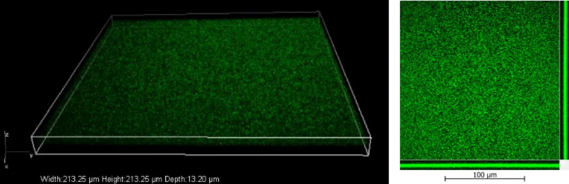
ORMOCER is delivered as a spincoated layer on top of a glass coverslip. Samples are supplied by our collaborators at the Fraunhofer Institute, group for Chemische Technologie der Materialsynthese, Sebastian Hasselmann. Us-ing a FEI Instruments ScannUs-ing Electron Microscope, we scanned the surface of an ORMOCER sample, see figure 5. We observed that it is homogeneous up to 10nm, at which scale the artifacts of Pt/Pd sputtercoating (‘cracks’) are visible on the surface. The figure on bottom-right shows an imperfection in the surface of about 500nm size. In the sample we investigated, we found less than 1% of the surface to show these imperfections. We conclude that the ORMOCER spincoated layers are sufficiently flat for our goal.

(12)

Figure 5: ORMOCER spincoated substrate under SEM.

(13)

3.2.3 Layer by Layer Polymer Supports

The polymer layer (as described by Decher et al. [9] and used by K¨ugler and Knoll [15]) consists of three polyelectrolytes with alternating charges that are adsorbed on the substrate in a layer-by-layer fashion. This process takes place in a 150mM NaCl 3mM NaN3 salt solution in MQ water. The polymers (PEI(+), PSS(-) en PAH(+), see table 1) are dissolved in this salt solution and brought to pH 5.5 using either NaOH or HCl. The pH is measured with a HACH PH17-SS Micro ISFET pH probe. The concentration of the polymers varies between experiments, see section 3.4. The substrate is first exposed to PEI solution. The PEI polymers are attracted by the negativity of the substrate (partially ionized SiOx groups) in the substrate.

The polymers saturate the surface in such a way, that the charge of the surface is effectively inversed (− →+) after the absorption: Per negative charge on the surface, two PEI+ _{monomers attach [9]. After at least 20 minutes, excess} PEI (in solution) is washed from the surface and the surface is exposed to PSS solution. The PSS couples electrostatically to the PEI groups and saturates the surface, thereby inversing its charge again (+ → −). After at least 20 minutes, excess PSS is washed from the sample and PAH solution is added. The positively charged PAH saturates the surface, etc. The amount of PSS/PAH layers that are absorbed on top of the PEI layer is indicated with the letter N. A schematic picture of this process is shown in figure 7.

(ORMOCER) PTA substrate PSS (-) PAH (+)

PEI (+)

Substrate (-)

N×

Lipid Bilayer

(14)

3.2.4 Lipid Bilayers in the Lab

To experimentally create a lipid bilayer, extrusion is used. The desired com-bination of lipids (dissolved in chloroform) is put in a microtube and dried in a vacuum desiccator at 1-5 mbar for at least 2 hours. After drying, 250 µLof salt solution (see previous paragraph) is added to the microtube. This brings the lipid concentration to 2g/L. The solution is vortexed for 10 minutes to allow the lipids to disperse in the salt solution. After that, we make small unilammelar vesicles (SUVs) using the Avanti Mini-Extruder®, see figure 8. The Mini-Extruder consists of two oppositely mounted 250µL syringes. The syringe needles enter the cell in the middle of the extruder. In this cell, two polycarbonate membranes with 30nm pore size are held between the two syringes by two filter supports, embedded in teflon support holders. An exploded view of the Mini-Extruder is shown in figure 8. By pushing lipid solution through the membrane the lipids form SUVs.

(15)

Before use, the needles of the extruder are washed with ethanol (once), MQ water (5 times) and salt solution (5 times). Then one needle is filled with 250 µL of salt solution and flushed though the extruder by pushing on the plunger of the needle. The salt solution flows through the cell of the extruder and into the other needle on the opposite site. This needle is emptied and we flush the extruder another two times with salt solution.

After the cleaning, a needle is filled with the lipid solution (250µL). This solution is transfered slowly through the membrane, into the other syringe. This movement is reversed and repeated 20 times. The lipids have now as-sembled into SUVs. We observe that the SUV solution is clear compared to the cloudy lipid solution. On average 200 µL of SUV solution is obtained from 250 µLof base solution due to losses in the extruder’s membranes.

To obtain lipid bilayers on substrates (such as polymer layers), we exploit a vesicle’s property to rupture: Upon contact with the substrate, the SUV bursts open and its constituent lipids form a bilayer on the substrate. This fusion is showed schematically in figure 9.

(16)

3.2.5 Sample Holder

To expose a substrate to a polymer support, we need a specific sample holder. The design of the sample holder has evolved over the course of this research. The main parts of the sample holder are a teflon ring (inner diameter 14mm, outer diameter 20mm, thickness 3mm), the substrate (glass of ormocer slide) and an adhesive to stick the ring on the substrate-slide. Teflon was chosen for its non-reactive nature, ensuring that it does not influence the experi-ments and making it easy to clean with acetone or ethanol. We tried various adhesives and found which work best.

Grease

In the first experiments we used Apiezon M vacuum grease (see table 1) as an adhesive. By putting grease on one side of the teflon ring, and pressing this side on the slide, a watertight seal between the teflon and the substrate forms and a reaction chamber for the experiments is created. However, when working with pipets in the reaction chamber, the teflon ring is easily moved from its position, particularly at higher temperatures (>22◦C) in the lab, when the grease is more fluid. We abandoned this design.

Tapes

In following experiments we used tapes. We discovered however that due to the use of tape, the experiment is influenced. In some experiments, a lipid bilayer did not form properly. We do not know if the polymer layers are also effected. Furthermore, the adhesive components of the tape turn out to be fluorescent. This impaired accurate imaging of the samples. In table below the tested tapes are listed together with our observations. Based on these observations, using tapes was abandoned.

Tape name (com-mercial

Conrad prod.nr.

Glue component Observations

ScotchTM _Ruban

Ad-hesive (3M 9527)

549370 Synthese

Kautschuk

Leaking of fluorescent ma-terial

ScotchTM Ruban

Ad-hesive (3M 9088)

549646 Modif. Acrylat Effects the formation of

the lipid bilayers 3M Power Klebeband

(8888195)

547829 Acrilaat Was not suitable: too

(17)

Paraffin

To solve the problems with the grease and the tapes, we used paraffin to stick the teflon ring to the sample. We choose paraffin for its non-reactiveness and purity of product. The design of the teflon rings was adapted: a 1*1mm

trench is milled on one side of the ring, see figure 10. Paraffin (melting point 52-54◦C) is heated on a hot plate to 80◦C. A 100µL pipette-tip is heated in a waterbath on the same hot plate. Once the pipette-tip is hot, it is used to pour 90µL of liquid paraffin into the trench. The volume of the trench is less than 90µL, forcing the paraffin to form a convex meniscus. Then the (room temperature) substrate is pressed on the ring, with the trench facing the substrate. The paraffin solidifies upon impact with the substrate and forms a seal. In ensure full waterproofing, more paraffin is added around the ring. Figure 10 shows the final product. We did not yet experience problems with this design of sample holder.

(18)

3.2.6 Microscopy

Samples were imaged using two microscopy techniques: Laser scanning con-focal microscopy and bright field microscopy. A NIKON TiE fully motorized inverted microscope with A1R confocal scanhead enables both techniques. Using the NIS elements software, images or image sequences can be saved and analyzed. With this scanhead, samples can be imaged in both resonant and galvano mode. We use resonant mode for z-stacks and galvano-mode for stimulation experiments. We use a 60x PLAN APO VC water immersion objective to image our samples.

Principle of Confocal Microscopy: 3D Image Acquisition

The principe of confocal microscopy is shown in figure 11. In confocal laser scanning microscopy, lasers are used to excite a small volume in the specimen (red lines in picture). In this volume, fluorescent molecules (dyes) are excited. These molecules then emit photons at a different wavelength (blue lines in picture). This light passes through an aperture (pinhole) before it reaches the detector. Out of focus signal (dotted gray line in picture) does not pass the pinhole. The pinhole causes the signal-strength to decay, since as a consequence only a very small portion of light passes through the pinhole. This explains the use of lasers: One needs a strong light source to counter the loss of signal caused by the pinhole. By line-scanning the lasers over the focal plane, an image is constructed. Using a piezoelectric z-stage, scanning over various focal planes is possible. These image-series (called a z-stack) can be combined to create a 3D picture of the specimen.

(19)

Lasers and Dyes

The dyes with corresponding laser and detector used in this research are listed in table 2.

Dye Excitation Maximum (nm)

Emission Maximum (nm)

Color Laser wavelength (nm)

Detector wavelength (nm)

NBD 458 530 Green 488 500-550

FITC 495 525 Green 488 500-550

6FAM 495 520 Green 488 500-550

Rhodamine 560 583 Red 561 565-625

Table 2: Dyes, lasers and detectors used in this research.

Z-stacks and representations

In figure 12, a z-stack of images of plain ormocer is shown in two presenta-tions: the volume view and the slices view. In this report the slice represen-tation with maximum intensity projection will be used to show z-stacks of images. MIP shows at each coordinate the brightest pixel of all constituent z-stacks at that coordinate. This representation gives most information about the substrate: The (x,y) slice shows inhomogeneities in the plane of the sub-strate, where the (y,z) and (x,z) planes show out-of-plane inhomogeneities on substrates/lipid bilayers.

100 {m

(20)

3.3 Theory

3.3.1 Lipid Bilayers and Lateral Diffusion

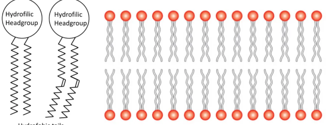
Lipid bilayers consist of individual lipids. Most lipids have two hydrophobic, fatty acid hydrocarbon tails and one hydrophilic headgroup. The hydropho-bic tails, which are repelled by water, are forced to aggregate when dissolved in a water-like solution. Bilayers are stable structures formed by clusters of lipids. In a lipid bilayer, the hydrophilic headgroups points outwards, into the solution, and the hydrofobic tails line up [31]. A picture of a lipid double layer (bilayer) is shown in figure 13.

In 1972, Singer et al. [24] published a famous article in which they formu-late the described composition of the lipid bilayer (cell membrane). Singer et al. argue that a lipid bilayer can be viewed as a two-dimensional liquid, in which the constituent lipids can freely diffuse. One could also say that a membrane is an anisotropic structure: it is ordered in the z-direction (per-pendicular to the surface) but disordered (mobile) in the x- and y-directions parallel to the surface. Fairly recent, it became possible to track single par-ticles diffusing in a lipid bilayer [21], see figure 14. This showed that single (fluorescent-marked) lipids diffuse freely in the x- and y- direction of a lipid bilayer. We call this form of diffusion, ‘lateral diffusion’

(21)

Hydrofilic Headgroup

Hydrofobic tails Hydrofilic Headgroup

Figure 13: Left: Schematic picture of a saturated (left) and an unsaturated (right) phospholipid. Right: Schematic cross section of a lipid bilayer. Lipids can diffuse freely in the horizontal direction. Figure from [32].

(22)

3.3.2 Mobility Measurements: FRAP

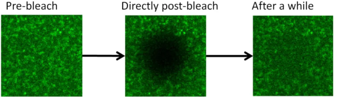
To determine the fluidity of the lipid bilayer, we do Fluorescent Recovery After Photobleaching (FRAP) experiments. We bleach a selected circular area (Region of Interest (ROI), typical radius 2-4 µm) in the plane of the lipid bilayer by scanning it at maximum laser power for approximately 1 second. If the lipid bilayer is fluid, lipids diffuse laterally in and out of the bleached area, causing recovery of the fluorescence in the bleached region. By analyzing this recovery, the diffusion coefficient of the lipid bilayer is extracted. In this section we will explain all details of this method. In figure 15, images from a FRAP experiment on a DOPE-NDB doped lipid bilayer on glass are shown to illustrate the concept.

Figure 15: FRAP: bleaching and recovery of a spot.

We define F1(t) as the mean signal intensity of the bleached ROI 1 and

F2(t) as the mean signal intensity of ROI 2, which serves as a reference to correct for background bleaching during the measurement. These ROIs are shown in figure 16a. The recovery curve FR(t) is defined as FR(t) = _FF1₂(₍t_t)₎.

(23)

(a)

0 5 10 15 20 25 30 35

Time(s) 0 200 400 600 800 1000 1200 1400 F1 ( t ) /F2 ( t )

F1(t)

F2(t)

0.0 0.2 0.4 0.6 0.8 1.0 1.2 FR ( t ) (b)

Figure 16: Figure (a) shows ROI 1 and ROI 2. Figure (b) shows F1(t), F2(t) and FR(t) in a typical FRAP experiment.

Quantitative analysis of FRAP experiments

In 1976, Axelrod et al. published an article [3] in which FRAP is introduced and a quantative connection is established between the recovery of the signal and the diffusion coefficient. Although others improved on their approach [27] [33], we will use Axelrods’ analysis as it is our goal to determine if the lipid bilayer is fluid, and to get a crude estimate of the diffusion coefficient. Axelrod assumes that the bleached spot is circular in shape and that the first measurement of the fluorescence of the spot after bleaching can be ap-proximated by a Gaussian profile. These assumptions are met by setting our ROI 1 as circular and setting the radius of the bleached spot below 3µm (as shown in [4]), respectively. Under these assumptions the diffusion coefficient is given by:

D= 0.22w 2

τ1 2

(1)

With D the diffusion coefficient, w the radius of the bleached spot, τ1 2 the

(24)

To extract τ1

2, we assume exponential recovery

1 _{of the fluorescence} fol-lowing [18]. We fit our data using a non-linear least squares fit to a three parameter exponential model as follows:

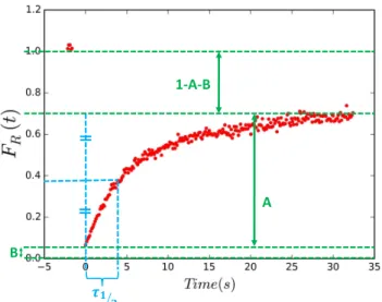
FR(t) = A(1−e−t/τ0) +B (2)

A graphical interpretation of parameters A, B and τ1

2 is shown in figure

17. We can physically interpret A+B as the maximum (asymptotic) re-covery the sample can achieve. In most FRAP experiments FR(∞)6= 1, i.e.

fluorescence recovery is seldom 100%. This is generally caused by an immo-bile contribution (the immobile fraction: 1−A−B) to the signal. We can interpret B as the offset in the recovery, caused by incomplete bleaching of the spot and/or a lag time between imaging and bleaching in which recovery already starts. We therefore translate our data to make recovery start at t=0. We can interpret τ1

2 as the time it takes for the fluorescence to recover

to half its asymptotic value. It is directly related to τ0 asτ1

2 =τ0·ln(2).

1-A-B

𝝉𝟏

𝟐

B

A

Figure 17: Data from FRAP experiment with graphical interpretation of A,B and τ1

2

.

1_{Please read ‘A note on the fitting procedure’ at the end of this chapter on the choice}

(25)

For fitting we define a cutoff FR(t) = α above which data will not be

used in the fit. The reason for this is that the fit generally underestimates the value of FR(t) at larger lag times. For this fit, α = 0.5 or cutoff = 50%

as shown. From our fit we calculate τ1

2 and the diffusion coefficient. These

are printed in figure 18.

5 0 5 10 15 20 25 30 35

Time

(

s

)

0.0 0.2 0.4 0.6 0.8 1.0 1.2

F

R

(

t

)

data

&

F

R

(

t

)

fit

radius

=3

.

5 µm

τ

h

=3

.

3 seconds

D

=0

.

8 µm

2

_/s

Cutoff

=50%

Original data Fit

Figure 18: Recovery curve as shown in figure 17 with fit.

To calculate the error inD, we need the errors inτ1

2 andw. We estimate

the error in τ1

2 to be a lot smaller than the error in w, as w is estimated

manually from the first post-bleaching image. We assume an error of 15-20% in w. Using the propagation of error method:

δD D 2 = 2 δw w 2 + δτ 1 2 τ1 2 !2 ≈2 δw w 2 (3) δD D = √ 2 δw w

(26)

A note on the fitting procedure

We remarked that an exponential recovery was assumed to extractτ1

2

follow-ing [18]. An different publication [34] replaces the exponential recovery with a fraction while keeping the physical interpretation of A, B and τ1

2 intact:

FR(t) =A





t τ1 2

1 + _τt

1 2



+B (5)

The diffusion coefficient is extracted with the same formula as before (equa-tion 1). This use of the frac(equa-tion motivated by experimental observa(equa-tion of

a linear relation between FR(t) and

t τ1 2

/

1 + _τt

1 2

in systems were only

lateral diffusion causes fluorescent recovery. We fitted our data (without cutoff) with this formula and found the agreement with our data to improve compared to the exponent, but the differences in extracted diffusion constant to be insignificant for most datasets. For datasets with very slow recovery however (such as shown in figure 37b) the results with the fraction-model gave unphysical results as A= 1.3 for this case. Based on this, we will stick with the exponential recovery to extract τ1

(27)

3.4 Results and Discussion on Polymer Supports

3.4.1 Introduction

In this section the experiments on creating a polyelectrolyte lipid bilayer support will be described. To be able to observe the polymer layers, we syn-thesized PAH·FITC. The synthesis protocol can be found in section 3.2.1. In the layer-by-layer deposition of the samples, we varied three parameters and investigated their influence on the homogeneity of the final polymer layer (PAH·FITC) as defects in this layer will cause defects in the supported lipid bilayer and thus inhibit free diffusion. We varied the number of layers (from N=2 to N=12), the substrate (glass or ORMOCER) and the polymer con-centrations in the solution (2 g/L or 50 g/L). The experimental method can be found in section 3.2.3. We will show our results per varied parameter.

(28)

3.4.2 Number of Layers (N)

An ORMOCER spincoated slide was dipped in 2 g/L solutions of the PEI, PSS of PAH. As final layer, we added PAH·FITC . Samples with N=2, N=4, N=8, N=10 and N=12 were created in this fashion.

100 {m 100 {m 100 {m

alfa 100 {m

B

100 {m

(a) N=2, HV=67

100 {m 100 {m 100 {m

100 {m

B

100 {m

(b) N=4, HV=59

Figure 19

(29)

100 {m

gamma

100 {m

beta

100 {m

alfa 100 {m

B

100 {m

(a) N=8, HV=40 100 {m

gamma

100 {m

beta

100 {m

alfa 100 {m

B

100 {m

(b) N=10, HV=40

100 {m

gamma

100 {m

beta

100 {m

alfa 100 {m

B

100 {m

(c) N=12, HV=40

(30)

From figures 19 and 20, the following observations can be made.

We observe in figure 19 that although the High Voltage (Gain) is low-ered the intensity increases, similar to figure 20, where we observe an

increase in brightness atequal settings.

In both figures 19 and 20, we observe an increase in objects sticking out of the PAH layer when the number of layers in increased. Large aggregates of polymer seem to form on top of the polymer layers as the number of layers increases. This is best visible in the (x,z) and (y,z) planes

(31)

3.4.3 Polymer Concentrations and Substrates

Inspired by a second publication by K¨ugler and Knoll [16], we increased the concentration of polymer in the polymer solutions from 2 g/L to 50 g/L. We experimented with these higher concentrations on both glass and ORMO-CER. It has to be remarked that the final layer (PAH·FITC) had a concen-tration of 2 g/L as it was synthesized at this concenconcen-tration. The number of layers (N) is 4.

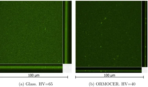
In figure 21, the results are shown for samples that were washed 3× be-fore imaging. In figure 22, the same samples are shown, however, now they were washed 10×.2

100 {m

zeta_005

100 {m

eta_002

100 {m 100 {m

(a) Glass. HV=75

100 {m

zeta_005

100 {m

eta_002

(b) ORMOCER. HV=55

Figure 21: These samples were cleaned three times before imaging.

2_{The images shown in figure 22 were taken after the polymer support was not only}

washed 10×, but also exposed to a lipid bilayer (see section 3.5). This particular lipid bilayer was rhodamine doped and therefore it does not interfere with our measurement of

the PAH·FITC. We assume that the washing caused all the difference between figures 21

and 22.

(32)

100 {m

zeta_005

100 {m

eta_002

100 {m 100 {m

zeta_w_lipids_001 eta_w_lipids_001(a) Glass. HV=65

100 {m

zeta_005

100 {m

eta_002

100 {m 100 {m

zeta_w_lipids_001 eta_w_lipids_001

(b) ORMOCER. HV=40

Figure 22: These are the same samples as in figure 21, but then washed 10×

before observation.

From figures 21 and 22, the following observations can be made.

Looking at the gain (HV) values in both figures 21 and 22, we observe that these are generally lower for the ORMOCER samples than for the glass samples, while the samples appear to be just as bright. This indi-cates that the ORMOCER samples give a stronger fluorescent signal. This is probably related to the fluorescence of ORMOCER itself, which has its emission maximum in the same range as FITC. This gives an offset to the signal.

Looking at the homogeneity using the (x,z) and (y,z) planes of figure 21 shows two things: Their are more inhomogeneities, but these inho-mogeneities seem less rooted in the surface than in for example figure 20c.

(33)

In correspondence with our observations in figures 19 and 20, the brightness of the images seem to decrease as homogeneity improves, however the gain also plays a role.

(34)

3.5 Results on Polymer Supported Lipid Bilayers

3.5.1 Introduction

After preparing a homogeneous polyelectrolye support, adding lipids to the polymer support is the next step. In this section our experiments on Polymer Supported Lipid Bilayers (PSLB) are described. Our aim is to create a

homogeneous andfluid lipid bilayer. Based on [15] we will turn our attention to four parameters:

1. The substrate: we want to use ORMOCER, but in the reference, glass is used. We will show our results on both substrates.

2. The final polymer layer: PAH+ _{or PSS}−_{. Kugler and Knoll are not}

specific about which layer is the final layer. We will thus try both. 3. The composition of the lipids; in the reference, the authors use 10%

negative lipids (DMPG) in their bilayer. We will try this too.

4. The lipid-attached dye. For reasons that will be explained, we looked at the difference between headgroup-labeled and fatty-acid labeled flu-orescent lipids.

(35)

3.5.2 Role of substrate

In figure 23 we show the same samples as in section 3.4 (figure 22) how-ever we exposed the polymer support to 0.125 g/L SUV solution. The lipid composition in this specific experiment is listed in table 3. In figure 24, we show three images from a FRAP experiment (see section 3.3.2) on the glass substrate PSLB.

Lipid Mass %

DOPC 97.8

DOPE-Rho 0.2

DSPE-Cap-Biotin 2

Table 3: Lipids used in experiments on role of substrate

100 {m 100 {m

(a) Glass

100 {m 100 {m

(b) ORMOCER

(36)

t=0s t = 5s t= 204 s

Figure 24: FRAP experiment on glass substrate PSLB. A square is bleached. The green spherical object in the right corner is a colloidal particle which is stuck on the lipid bilayer. The colloid has a diameter of 1µm.

From figures 23 and 24, we observe the following:

In figure 23a we only observe a few artifacts in the lipid bilayer. Upon close comparison with figure 22a it is observed that on polymer layer defects, larger lipid bilayer defects are formed.

The ORMOCER substrate PSLB however is less homogeneous than on the glass substrate. Large lipid artifacts form on the surface of this polymer support. Comparing with 22b, we observe that although the PAH·FITC endlayer seems to be relatively homogeneous, the lipids don’t fuse homogeneously on the surface.

In figure 24 we show the results of a FRAP experiment on the glass PSLB from figure 23a. We do not observe any fluidity of the lipid bilayer up to 200 seconds recovery.

We conclude that we are able to create a homogeneous PSLB on glass. This lipid bilayer is however not fluid. To create a fluid lipid bilayer in fol-lowing experiments, we will focus on the role of the final polymer layer and composition of the lipid bilayer in the next paragraphs.

(37)

3.5.3 Role of Negative Lipid and Final Polymer Layer

Based on [15], in which the authors demonstrate a mobile PSLB using 10% negative lipid (DMPG), we made SUVs with 10 mass% DOPG (also neg-ative). At the same time we test the influence of a different final polymer layer: PAH+ _{or PSS}−_{. We used DOPE-NBD as a dye; DOPE-NBD is easier}

to bleach that rhodamine, making it more suitable for FRAP experiments. The exact lipid composition is shown in table 4. We exposed the polymer supports to 0.28 g/L SUV solution.

Lipid Mass %

DOPC 88

DOPG 10

DOPE-NBD 1

DSPE-Peg-Biotin 1

Table 4: Lipids used in experiments on role of negative lipid

200 {m

PAH final layer sample 2 18-06-2015 z-stack 001

50 {m

PSS final layer sample 3 18-06-2015 z-stack 001

(a) PAH+ final layer

200 {m

PAH final layer sample 2 18-06-2015 z-stack 001

50 {m

PSS final layer sample 3 18-06-2015 z-stack 001

(b) PSS− final layer

(38)

t=0s

t = 2s

t= 8 s

5 μm

_{5 μm}

(a) PAH+ final layer

t=0s

t = 2s

t= 8 s

5 μm

(b) PSS− final layer

(39)

From figures 25 and 26, we observe the following:

On both negative and positive final polymer layers, 10% negative lipid SUVs form a bilayer.3

The lipid bilayer formed on the PAH+ _{support is much less} homoge-neous than the lipid bilayer formed on the PSS−. The lipid bilayer formed on PSS− is very homogeneous.

Both lipid bilayers are not fluid.

We can conclude that although the lipid bilayer formed homogeneously on the PSS− final layer polymer support, no mobility in this bilayer is observed. The 10 mass% negative lipids were not fluid either.

3_{One would expect an inhibition of rupture of negatively charged SUV’s on a PSS}−_final

(40)

3.5.4 Role of the Dye

In the previous experiments we used DOPE-NBD. This is a negatively charged fluorescent lipid with the dye attached to the headgroup of the lipid. We suspected that the dye might be influenced by the polymer layers as the neg-ative lipid is either pulled towards or pushed away from the charged polymer support. A FRAP experiment, in which solely the lateral diffusion of the

dye-attached lipids is probed (the other lipids are not observed by confocal microscopy), might therefore not represent the actual mobility of the lipid bilayer. To investigate this hypothesis, we exchanged the DOPE-NBD for PC-C6-NBD. PC-C6-NBD is neutral and has the same headgroup as DOPC. It is therefore a better probe for fluidity.

In the following experiments, a lipid bilayer with constituent lipids listed in table 5 is fused on a PSS (N=3.5) and a PAH (N=2) final layer sample.

Lipid Mass %

DOPC 89

DOPG 10

PC-C6-NBD 1

Table 5: Lipids used in experiments on the role of the dye

50 {m 50 {m

14C_z-stack_002 washed PAH final layer

14B_z-stack_001 washed PSS final layer

(a) PAH+ final layer, HV=67

50 {m 50 {m

14C_z-stack_002 washed PAH final layer

14B_z-stack_001 washed PSS final layer

(b) PSS− final layer. HV=80

(41)

t=2s

t = 4s

t= 22s

5 μm

_{5 μm}

(a) PAH final layer

t=5s

t = 6s

t= 120 s

5 μm

(b) PSS final layer

Figure 28: Lipids with PC-C6-NBD are fused on a PAH+(a) and a PSS−(b) substrate.

(42)

3.6 Conclusion on Polymer Supported Lipid Bilayers

In the last two sections, we presented our results on polymer support lipid bilayers. We studied the polymer supports separately by visualizing the final polymer layer in the confocal microscope. We studied the homogeneity of this final layer as a function of the number of layers (N) and the polymer concentration in the solutions. We concluded that at high polymer concen-trations, homogeneous final layers are formed when proper washing is applied to the sample to remove excess polymer aggregates from the surface. This holds for both glass and ORMOCER substrates.

We investigated the effect of the substrate on lipid bilayer formation and observed that even when the final polymer layer appears homogeneous, a difference in bilayer coating arises: On glass a homogeneous bilayer forms, but on ORMOCER the layer is inhomogeneous. We investigated the role of negative lipids, final polymer layer and the dye on the fluidity of a glass-substrate PSLB, but we not able to create fluidity.

(43)

K¨ugler and Knoll Experiments presented in this thesis

Substrate Functionalized SiOx(glass) Glass or ORMOCER

Substrate cleaning Unspecified Hellmanex, ethanol

Salt solution Unspecified buffer or MQ 150mM NaCl 3mM NaN3

Polymers PEI, PSS, PAH PEI, PSS, PAH

Concentration Not clear 2g/L and 50 g/L

pH 5.4 or MQ 5.4±0.5

Absorption Time 20 minutus 20-30 minutes

Number of Layers (N) 4 2-12, usually 4

Final layer Not fully clear Tried PAH or PSS

Lipids

Composition 90% DMPC 88% DOPC

10%DMPG 10% DOPG

?% PC-C4-NBD 1%PC-C6-NBD

(1% DSPE-Peg-biotin)

SUV technique Extrusion Extrusion

SUV concentration on absorption

Not mentioned ≈0.1 g/L

Adsorption Time Up to multiple hours 30 min up to multiple hours

(44)

3.7 Results on Glass/ORMOCER Supported Lipid

Bi-layers

3.7.1 Experimental Goal II: Fluidity

Because we were unable to achieve a mobile lipid bilayer on a polymer sup-port, we decided to use the method in [7] to obtain a fluid bilayer. Starting with glass substrates, we can go towards ORMOCER. We studied the effect of the lipid composition on the fluidity of lipid bilayers on glass and ORMO-CER, as shown in table 7.

In previous experiments, we tried to minimize the contribution of the sub-strate by experimenting with a polymer interlayer build up of multiple layers of PEI, PSS and PAH (see section 3.5). We could not get the lipid bilayer fluid on top of these layers. In order to minimize the contribution of OR-MOCER we will now incorporate the polymer cushion (steric stabilitzation) in the lipid bilayer itself by using DOPE-PEG2000 or DPPE-PEG2000.

Parameter Range/Value

Lipid compositions Role of negative lipids [DOPG]: 0 and 10 Mass%

Role of PEG [DOPE-PEG]: 0 and 10 Mass%

[DPPE-PEG]: 0 and 10 Mass%

Dyes DOPE-Rho

DOPE-NBD

Other varied parameters Substrate Clean glass or ORMOCER

Salt solution 150mM NACl 3mM NaN3in MQ

or 150mM NaCl HEPES in MQ

(45)

3.7.2 Results on Glass

In this paragraph, experiments on glass supported lipid bilayers are de-scribed. First we will describe an experiment with pure DOPC lipids (99.8%). Then we will schematically show our results on other lipid compositions.

Example: Pure DOPC lipids

The following lipid composition was used:

Lipid Mass %

DOPC 99.8

DOPE-Rho 0.2

We exposed a clean glass surface to 0.26 g/L SUV solution. The sample is not washed before observation. In figure 29 a z-stack of the surface is shown. In figure 30 we show the raw data from the FRAP-experiment. In figure 31 the analysis of the experiment is shown as explained in section 15.

200 {m

Figure 29: Z-stack of glass supported DOPC lipid bilayer.

(46)

Figure 30: Sequence of images from the FRAP experiment show the moment of bleaching and the recovery of fluorescent signal.

2 1 0 1 2 3 4 5 6 7

Time

(

s

)

0.4 0.5 0.6 0.7 0.8 0.9 1.0 1.1

F

R

(

t

)

data

&

F

R

(

t

)

fit

radius

=2

.

0 µm

τ

h

=0

.

5 seconds

D

=1

.

9 µm

2

_/s

Cutoff

=85%

Original data

Fit

(47)

Results with other compositions of lipids

We repeated our FRAP experiments on glass supported lipid bilayers using other compositions of lipids. We tested lipid compositions with 10 mass% DOPG (negative lipid), as well as lipid compositions with 10 mass% DOPE-PEG2000/DPPE-PEG2000.

We present the results on glass supported lipid bilayers in table 8. Sample 1 is shown in the previous paragraph. Sample 3 and 4 show two values for D, originating from two FRAP experiments in the same sample. As explained in section 15, the relative error in D is 25%.

Figure Lipid composition (mass %)

Washed? Lipid concen-tration (g/L)

Cutoff D (µm2_/s₎

31 DOPC:DOPE-Rho

99.8:0.2

No 0.26 90% 1.9

36a DOPC:DOPG:

DOPE-NBD 89:10:1

Yes 0.29 90% 0.8

36b 36c

DOPC:DOPE-PEG: DOPE-Rho 89.9:10:0.2

Yes 0.15 90% 1.1

1.1 36d

36e

DOPC:DPPE-PEG: DOPE-Rho 89.9:10:0.2

Yes 0.15 90% 1.3

1.3

Table 8: Results of FRAP experiments on glass supported lipid bilayers. Figure 36 can be found in section 3.7.5.

(48)

3.7.3 Results on ORMOCER

Having established fluid lipid bilayers on a clean glass support, we investi-gated the mobility of these same lipids on ORMOCER.

PEG2000: Revival of polymer cushion

Using DOPE-PEG2000 and DPPE-PEG2000, we achieved mobile lipid bi-layers on ORMOCER. In the table below, our results are presented.

Figure Lipid composition (mass %)

Washed? Lipid concen-tration (g/L)

Cutoff D (µm2_/s₎

N.A. DOPC:DOPG:

DOPE-NBD 89:10:1

Yes 0.15 No

mo-bility

37a DOPC:DOPE-PEG:

DOPE-Rho 89.9:10:0.2

Yes 0.15 60% 0.08

37b DOPC:DPPE-PEG:

DOPE-Rho 89.9:10:0.2

Yes 0.15 40% 0.01

Table 9: Results of FRAP experiments on ORMOCER supported lipid bi-layers. Figure 37 can be found in section 3.7.5.

(49)

3.7.4 Appendix I: Other observations

In this section we describe some observations made while experimenting on glass and ORMOCER supported lipid bilayer. Hopefully these observation prove helpful in the follow up research on this topic.

Fluidity in Sonicated Lipids

Following [6], we tried sonication as an alternative to extrusion. In sonication, the lipids are agitated at frequencies>20kHz in an ultrasonic bath for approx. 1 hour. The difference between sonicated lipids and extruded lipids is shown in figure 32. We observe that sonicated lipids form a cloudier solution. This indicates more or bigger lipid aggregates.

Figure 32: Extruded and sonicated lipids side by side.

(50)

0.3 sec 1.1 sec 15 sec Homogeneous region

Inhomogeneous region

5 μm

5 μm 5 μm

5 μm

5 μm 5 μm

Figure 33: Homogeneous and inhomogeneous regions found in a sample made with sonicated lipids.

Fluidity on 3D structures

As shown in figure 5, defects in ORMOCER can be present. During our ex-periments on ORMOCER supported lipid bilayers (lipid composition: DOPC: DPPE-PEG: DOPE-Rho 89.9:10:0.2), we found a large defect. We observed that this defect was very well covered with lipid bilayer (strong signal) and

(51)

After 1 min

After 2 min

(52)

Critical Parameters: Lipid Concentration and Fusion Time

In one of our experiments on glass supported lipid bilayers, we used a 0.08g/L SUV solution to coat the substrate and impatiently imaged the sample after only 15-30 minutes. We observed no fluidity. After increasing the SUV con-centration to 0.29 g/L we did observe fluidity! However, the recovery was not 100%, but small islands of non-fluorescence were found in the ROI after recovery. This indicated that the sample was not sufficiently covered with lipid bilayer: In some areas the lipid bilayer was not attached to the ‘main patch’ so it could not recover after bleaching. After another 15 minutes full recovery did occur. These observations are shown in figure 35.

We conclude that at least one hour fusion time should be taken before imag-ing and 0.26 g/ L of SUV solution definitely suffices. Later on we used 0.13 g/L in our experiments. This was enough when combined with 1 hour fusion time.

Pre-bleach Post-bleach Some time later Recovery curve

(53)

3.7.5 Appendix II: Graphs

In this section all graphs relating to the described FRAP experiments can be found.

5 0 5 10 15 20

Time(s)

0.2 0.4 0.6 0.8 1.0 FR ( t

)data

&

FR

(

t

)fit

radius=2.0µm

τh=1.1seconds

D=0.8µm2_/s

Cutoff=90%

Original data Fit

(a)

10 5 0 5 10 15 20

Time(s)

0.3 0.4 0.5 0.6 0.7 0.8 0.9 1.0 1.1 FR ( t

)data

&

FR

(

t

)fit

radius=2.0µm

τh=0.8seconds

D=1.1µm2_/s

Cutoff=90%

Original data Fit

(b)

10 5 0 5 10 15 20

Time(s)

0.3 0.4 0.5 0.6 0.7 0.8 0.9 1.0 1.1 FR ( t

)data

&

FR

(

t

)fit

radius=2.0µm

τh=0.8seconds

D=1.1µm2_/s

Cutoff=90%

Original data Fit

(c)

10 5 0 5 10 15 20

Time(s)

0.4 0.5 0.6 0.7 0.8 0.9 1.0 1.1 FR ( t

)data

&

FR

(

t

)fit

radius=2.0µm

τ_h=0.7seconds

D=1.3µm2_/s

Cutoff=90%

Original data Fit

(d)

10 5 0 5 10 15 20

Time(s)

0.4 0.5 0.6 0.7 0.8 0.9 1.0 1.1 FR ( t

)data

&

FR

(

t

)fit

radius=2.0µm

τh=0.7seconds

D=1.3µm2_/s

Cutoff=90%

Original data Fit

(e)

(54)

20 0 20 40 60 80 100 120

Time(s)

0.0 0.2 0.4 0.6 0.8 1.0 FR ( t

)data

&

FR

(

t

)fit

radius=2.0µm τh=11.0seconds

D=0.08µm2_/s

Cutoff=60%

Original data Fit

(a)

10 0 10 20 30 40 50 60

Time(s)

0.0 0.1 0.2 0.3 0.4 0.5 0.6 0.7 0.8 0.9 FR ( t

)data

&

FR

(

t

)fit _radius₌₂_.₀_µm

τh=66.0seconds

D=0.01µm2_/s

Cutoff=40%

Original data Fit

(b)

(55)

3.8 Conclusion on Lipid Bilayers

In section 3.7 we presented results on lipid bilayer coatings of glass and OR-MOCER. We observed that pure DOPC, DOPC:DOPG≈9:1, DOPC:DOPE-PEG2000≈ 9:1 and DOPC:DPPE-PEG2000 ≈9:1 lipid bilayers are all fluid on glass, with a diffusion coefficients≈1µm2_/s_{. We observed that in order to} obtain a fluid lipid bilayer on ORMOCER, we need to mix DOPE-PEG2000 or DPPE-PEG2000 lipids in the membrane ( DOPC:DOPE-PEG2000≈9:1). This presumably creates a supporting cushion between the ORMOCER sub-strate and the lipid bilayer. We observed that the diffusion coefficient for our lipid bilayers on ORMOCER ≈ 0.05 µm2/s

(56)

Figure Filename (.nd2)

6 20150430 PLAIN ORMOCER 001

15,16,17,18 20150702 12A with-linkers GREEN FRAP 002

19a 20150305 sample A 003

19b 20150305 sample B 002

20a 20150323 sample alfa 001

20b 20150323 sample beta 003

20c 20150323 sample gamma 002

21a 20150323 sample eta 002

21b 20150323 sample zeta 005

22a 20150323 sample eta with lipids 001

22b 20150323 sample zeta with lipids 001

23a 20150323 sample eta with lipids 001

23b 20150323 sample zeta with lipids 001

24 20150323 sample eta with lipids 003

25a 20150618 sample 2 z-stack 001

25b 20150618 sample 3 z-stack 001

26a 20150618 sample 2 FRAP 001

26b 20150618 sample 3 FRAP 001

27a 20150702 sample 14C washed z-stack 002

27b 20150702 sample 14B washed z-stack 001

28a 20150702 sample 14C washed FRAP 001

28b 20150702 sample 14B washed FRAP 001

29 20150702 sample 13B z-stack 001

30 20150702 sample 13A FRAP 001

31 20150702 sample 13A FRAP 001

33 20150615 glass sonicated lipids FRAP 010 (top) / 005 (bottom)

34 (top) 20150728 sample 22B washed z-stack 002

34 (others) 20150728 sample 22B washed FRAP 002 (middle) / 001(bottom)

35 20150604 sample I FRAP 001 (top) / 003 (middle) / 006 (bottom)

36a 20150529 sample 1 FRAP 002

36b 20150728 sample 21A washed FRAP 001

36c 20150728 sample 21A washed FRAP 002

36d 20150728 sample 22A washed FRAP 001

36e 20150728 sample 22A washed FRAP 002

37a 20150728 sample 21B washed FRAP 005

37b 20150728 sample 22B washed FRAP 004

(57)

4 PART II: The Two Dimensional Diffusion

of Colloids Attached to Fluid Lipid Bilayers

4.1 Experimental Goal

In this part of the report, an experimental effort to build the model system (see section 2) is described. A starting point follows from our conclusion of part I: A fluid lipid bilayer on both glass and ORMOCER is obtained when DOPC:DOPE-PEG2000≈ 9:1 and DOPC:DPPE-PEG2000 ≈ 9:1 lipids are used.

(58)

Glass / ORMOCER

Polystyrene (PS)

10% PEG2000 in Lipid Bilayer

NeutrAvidin

Biotin

Double stranded DNA

S’ sticky end with RITC dye

S sticky end with FITC dye

Double cholesterol anchor

(59)

4.2 Methods and Materials

Only materials and methods that are new will be described in this section. The other methods can be found in section 3.2. The file names of the raw data corresponding to the figures shown in this part of the report can be found in table 11, section 4.6, page 67.

4.2.1 DNA-Linkers and Colloids

The DNA linkers are formed from single stranded DNA with functionalized tail and head. These strands are specially designed following the recipe by [26]. The strands are synthesized by Eurogentec. The exact composition of the strands is shown in figure 39.

DNA linker in lipid bilayer:

Chol.-TEG-5’-TTT ATCGCTACCCTTCGCACAGTCAATCTAGAGAGCCCTGCCTTACGA-3’-S

Backbone: |||||||||||||||||||||||||||||||||||||||||||| Chol.-TEG-3’-TTT TAGCGATGGGAAGCGTGTCAGTTAGATCTCTCGGGACGGAATGC-5’

S sticky end: GTAGAAGTAGG-3’-6FAM

DNA linker on colloid:

Biotin-TEG-3’- TTT TAGCGATGGGAAGCGTGTCAGTTAGATCTCTCGGGACGGAATGC-5’ Backbone: ||||||||||||||||||||||||||||||||||||||||||||

Cy3 5’- TTT ATCGCTACCCTTCGCACAGTCAATCTAGAGAGCCCTGCCTTACGA-3’-S’

S’ sticky end: CCTACTTCTAC -3’

Figure 39: Composition of DNA linkers

To make the DNA linkers, the separate strands (from 100µM stock solu-tions) are dissolved in 45 µLof 10 mM PBS, 47 mM NaCl, 3 mM NaN3, pH 7.5 solution in a low-bind, PCR clean microtube. The backbone is hybridized by heating this solution to 90 ◦C and cooling down to room temperature at a rate of approx. 10◦C/hour.

To make the cholesterol DNA linkers 5µL ‘sticky’ strand and 7.5 µL ‘non-sticky’ strand are dissolved in PBS, bringing the molarity of hybrids to 4.34

(60)

The 1µmpolystyrene colloids (SFPS12) are synthesized following [2]. These colloids are Neutravadin coated using an EDC / Sulfo-NHS coupling reaction [12]. To attach DNA to these colloids, we add 200µg colloids and X pmol of DNA linkers to 310 µLof PBS buffer. By tuning X, particles with different linker concentrations are obtained, see table below. We incubate this solu-tion at 55◦C for 30 min and wash three times in HEPES by centrifuging and replacing the supernatant.

X (pmol) Linker density (linker / particle)

1.04 3.47×103

4.16 1.38×104

41.6 1.38×105

4.2.2 Assembly of the System

To assemble the system, we expose a substrate (ORMOCER or glass) to 0.15

g/Lof either DOPC:DOPE-PEG2000≈9:1 or DOPC:DPPE-PEG2000≈9:1 SUV solution in HEPES (amount of dye in SUVs<1%) for at least one hour. To check the formation of the lipid bilayer, we perform a FRAP experiment to determine the fluidity in this stage (‘Stage 1’). If we confirm fluidity, we wash the sample at least 5 times with HEPES and expose the surface to a 34 nM DNA linker solution for at least 30 minutes. The cholesterol groups on the linkers anchor in the lipid bilayer. We again perform separate FRAP experiments on both the lipid bilayer and the linkers (‘Stage 2’). We wash the sample at least 5 times if fluidity of both is observed. We add our DNA linker coated colloids to the sample to complete the system. The colloids are given at least one hour for their DNA linkers to couple with the complementary linkers in the lipid bilayers. We use bright field microscopy to observe diffusion of the colloids. If diffusion is observed, the fluidity of both the linkers and bilayer is confirmed via FRAP experiments in the area in which the colloid is diffusing (‘Stage 3’) as a check for the system.

4.2.3 Tracking

(61)

4.3 Diffusion in Two Dimensions

Colloids anchored to a 2D lipid bilayer experience Brownian motion. Follow-ing [10], the probability density of the particle displacement in two dimen-sions is given by:

P(r, t) = 1

4Dπtexp(

−r2

4Dt) (6)

Taking the second moment to calculate hr2iwe obtain:

hr2i= 4Dt (7)

Which relates the Mean Square Displacement (MSD) to the diffusion coefficient. We will use this formula to confirm the diffusion of colloids on bilayers.

4.4 Results and Discussion

4.4.1 High Linker Density: Mobility and Tracking

We exposed a glass substrate to the experimental steps described in section 4.2. We use DOPE-PEG2000 in this case with high linker density on the colloids (X = 41.6 pmol). In figure 40, data from the FRAP experiments on both the linkers and lipid are shown (stage 1 and 2). After adding colloids, we observed one colloid undergoing 2D diffusion. In figure 40d we show one image of this colloid, with its path superimposed in blue. We observed that in the region in which the colloid diffused, the lipid bilayer and linkers were both still mobile (stage 3). All other colloids in this sample were immobile; this means less than 0.1% of the colloids was mobile.

We plot the mean square displacement and observe that this scales linearly with the lag time, indicating that the particles exhibits Brownian motion, see figure 40e. We fitted the data up to the point (determined by eye) where the MSD starts to deviate from the linear relation as a result of the finite amount of data. We determine the effective diffusion coefficient of this colloid:

hr2i= 4Dt ↔D= hr

2_i 4t =

1

4·slope ≈0.04µm

(62)

5 0 5 10 15 20 25 30

Time(s)

0.3 0.4 0.5 0.6 0.7 0.8 0.9 1.0 1.1 FR ( t

)data

&

FR

(

t

)fit

D=0.9962µm2_/s

Cutoff=90%

Original data Fit

(a)

5 0 5 10 15 20 25 30

Time(s)

0.4 0.5 0.6 0.7 0.8 0.9 1.0 FR ( t

)data

&

FR

(

t

)fit

D=1.1413µm2_/s

Cutoff=90%

Original data Fit

(b)

5 0 5 10 15 20 25 30

Time(s)

0.0 0.2 0.4 0.6 0.8 1.0 1.2 FR ( t

)data

&

FR

(

t

)fit

D=0.7335µm2_/s

Cutoff=80%

Original data Fit

(c) (d)

5 10 15 20 25 30

lag time t (s)

0 1 2 3 4 5 6 ∆

r

2 ®

[

µm

2

]

Slope = 0.172 micron^2/s

Mean Square Displacement Linear Fit

(e)

(63)

4.4.2 Lower Linker Density on Colloid

In the previous section we show one diffusing colloid. We suspect the low amount of mobile colloids in this sample to be caused by the linker concen-tration: Contrary to theS linkers in the bilayer, theS’linkers on the colloid are immobile in the colloid surface. As the S and S’ linkers combine, the linker-pairs accumulate in the contact area until all S’ linkers on the colloid have an S partner. S linkers are excessively available and fresh linkers can diffuse into the contact area.

Increasing number of linker pairs per colloid likely decreases their mobil-ity as large linker-pair patches diffuse slower than individual linkers (which we probe in a FRAP experiment) and increased local cholesterol concentra-tion in the lipid bilayer decreases the mobility of the bilayer [11].

To test the influence of linker concentration, we lowered X to 1.06 pmol

(64)

(a)

(b)

Figure 41: Results with lower linker density on colloid

(65)

Mobility on ORMOCER

In figure 42 we show FRAP data of an ORMOCER substrate coated with lipid bilayer and exposed to DNA linkers as explained in section 4.2. Figure 42a and 42b show the FRAP data from the lipid bilayer (red fluorescent) and the linkers (green fluorescent) respectively. The partial recovery of the linkers is due to the permanent bleaching of the ORMOCER. When adding colloids we observe that they all get stuck.

10 0 10 20 30 40 50 60 70

Time(s) 0.1 0.2 0.3 0.4 0.5 0.6 0.7 0.8 0.9 1.0 FR ( t

)data

&

FR

(

t

)fit

radius=2.5µm

τh=3.3seconds

D=0.4195µm2_/s

Cutoff=85%

Original data Fit

(a)

50 0 50 100 150 200 250 300 Time(s) 0.2 0.0 0.2 0.4 0.6 0.8 1.0 FR ( t

)data

&

FR

(

t

)fit

radius=2.5µm

τh=20.7seconds

D=0.0663µm2_/s

Cutoff=40%

Original data Fit

(b)

(66)

4.5 Conclusion

(67)

4.6 Preliminary Experiments and Outlook

In the experiment with low linker concentration, we observe most (80-99%) of our colloids became stuck after contact with the lipid bilayer. Follow up research needs to look for ways to increase repulsion between the surface and the colloid. We would like to propose two experiments to increase repulsion by increasing the steric stabilization.

Increasing Steric Stabilization: PEG on Colloids and Lipid Bilayer

In preliminary experiments we added biotinylated PEG5000 to the colloids before incubation in a 10:1 PEG2000:DNA Linker molar ratio to increase the steric stabilization resulting from the interaction between the PEG in bilayer and on the colloid. Preliminary results did not produce diffusing colloids (they all got stuck), but the influence of factors as sample age or nuclease contamination on this result cannot be ruled out. Further investigation is needed.

Repulsion can also be increased by adding PEG5000 instead of PEG2000 to the lipid bilayer. The length of a PEG molecule scales with the square root of its molecular weight [35]. We estimate the length of PEG5000 molecule to be shorter than the DNA linker therefore providing stronger repulsion than PEG2000.

Outlook: 3D Substrates

When 2D diffusion of colloids can be accomplished for all colloids on glass substrates the next step is to use ORMOCER substrates. Based on our conclusion of part I, we expect diffusion to be slower on these substrates as the diffusion coefficients of lipid bilayers are generally lower on ORMOCER. This is not a fundamental problem as studying diffusion is also possible at low diffusion coefficients.

(68)

will refract the light beams (act as a lens), impairing the imaging. Fast z-stack acquisition in resonant confocal micropcopy might be an option.

Sample List

Figure Filename (.nd2)

40a 20150820 sample 21C FRAP 003

40b 20150820 sample 21C with-linkers FRAP RED 001

40c 20150820 sample 21C with-linkers FRAP GREEN 003

40d 20150820 sample 21C with-beads movie 001 crop

40e 20150820 sample 21C with-beads movie 001 crop

41a 20150825 sample 25A1 with-beads movie 002

41b 20150825 sample 25A1 with-beads movie 002

42a 20150722 sample 18A with-linkers red FRAP 002

42b 20150722 sample 18A with-linkers red FRAP 002

(69)

5 Acknowledgements

First of all I would like to thank my direct supervisor Casper van der Wel for your guidance and support during my master research project. Your great knowledge of experimental tools, microscopy, analysis and theory propelled this research and made my stay in the group a very instructive period. I would like to thank my supervisor Daniela Kraft; on one part for your ent-housiasm and insight in the project, but equally important, for proving the framework in which this research was conducted: An enthusiastic and profes-sionally organized research group that fosters creativity and a positive work environment. I would like to thank Indrani Chakraborty for all your help with the DNA linkers and many borrowed samples from linkers to colloids and SUVs. I would like to thank all members of the Soft Matter Physics group for good cooperation and the great I time had in this group!

(70)

References

[1] Boris N. Chichkov Andreas Ostendorf. Tpa printing, 2006.

[2] Jeroen Appel, Sabine Akerboom, Remco G. Fokkink, and Joris Sprakel. Facile one-step synthesis of monodisperse micron-sized latex particles with highly carboxylated surfaces. Macromolecular Rapid Communica-tions, 34(16):1284–1288, 2013.

[3] D Axelrod, DE Koppel, J Schlessinger, Ei Elson, and WW Webb. Mo-bility measurement by analysis of fluorescence photobleaching recovery kinetics. Biophysical journal, 16(9):1055, 1976.

[4] Kevin Braeckmans, Liesbeth Peeters, Niek N Sanders, Stefaan C De Smedt, and Joseph Demeester. Three-dimensional fluorescence re-covery after photobleaching with the confocal scanning laser microscope.

Biophysical journal, 85(4):2240–2252, 2003.

[5] Lukas Buehler. Cell membranes. Garland Science, Taylor and Francis Group, New York, NY, 2015.

[6] Nam Joon Cho, Lisa Y. Hwang, Johan J R Solandt, and Curtis W. Frank. Comparison of extruded and sonicated vesicles for planar bilayer self-assembly. Materials, 6(8):3294–3308, 2013.

[7] Paul S. Cremer and Steven G. Boxer. Formation and Spreading of Lipid Bilayers on Planar Glass Supports. The Journal of Physical Chemistry B, 103(13):2554–2559, 1999.

[8] J Crocker, J Crocker, and D Grier. Methods of Digital Video Mi-croscopy for Colloidal Studies. Journal of Colloid and Interface Science, 179(1):298–310, 1996.

[9] G. Decher, J.D. Hong, and J. Schmitt. Buildup of ultrathin multilayer films by a self-assembly process: III. Consecutively alternating adsorp-tion of anionic and caadsorp-tionic polyelectrolytes on charged surfaces. Thin Solid Films, 210-211:831–835, April 1992.

(71)

[11] Emma Falck, Michael Patra, Mikko Karttunen, Marja T. Hyvnen, and Ilpo Vattulainen. Lessons of slicing membranes: Interplay of packing, free area, and lateral diffusion in phospholipid/cholesterol bilayers. Bio-physical Journal, 87(2):1076 – 1091, 2004.

[12] Hans Fruijters. Directed self-assembly of tetrahedral particles. Master’s thesis, Universiteit Leiden, the Netherlands, 2015.

[13] K H Haas and H Wolter. Synthesis, properties and applications of inorganic-organic copolymers (ORMOCER (R) s). Current Opinion in Solid State & Materials Science, 4(1999):571–580, 1999.

[14] David Holcman and Antoine Triller. Modeling synaptic dynamics driven by receptor lateral diffusion. Biophysical Journal, 91(7):2405 – 2415, 2006.

[15] R K¨ugler and W Knoll. Polyelectrolyte-supported lipid membranes.

Bioelectrochemistry, 56(1-2):175–178, May 2002.

[16] Ralf K¨ugler, Johannes Schmitt, and Wolfgang Knoll. The swelling be-havior of polyelectrolyte multilayers in air of different relative humidity and in water. Macromolecular Chemistry and Physics, 203(2):413–419, 2002.

[17] Remy Kusters and Cornelis Storm. Impact of morphology on diffusive dynamics on curved surfaces. Physical Review E, 89(3):032723, March 2014.

[18] EMBL lectures. Frap analysis by embl, 2015.

[19] Avanti Polar Lipids. Avanti mini extruder, 2014.

[20] Marie-Paule Mingeot-Leclercq, Magali Deleu, Robert Brasseur, and Yves F Dufrˆene. Atomic force microscopy of supported lipid bilayers.

Nature protocols, 3(10):1654–1659, 2008.

[21] G J Sch¨utz, H Schindler, and T Schmidt. Single-molecule microscopy on model membranes reveals anomalous diffusion. Biophysical journal, 73(2):1073–1080, 1997.

(72)

[23] Sigma-Aldrich. Pah, pei and pss structural formulas, 2015.

[24] S. J. Singer and Garth L. Nicolson. The fluid mosaic model of the structure of cell membranes. Science, 175(4023):720–731, 1972.

[25] Motomu Tanaka and Erich Sackmann. Polymer-supported membranes as models of the cell surface.Nature, 437(7059):656–63, September 2005. [26] Stef A. J. van der Meulen and Mirjam E. Leunissen. Solid colloids with surface-mobile dna linkers. Journal of the American Chemical Society, 135(40):15129–15134, 2013. PMID: 24040916.

[27] Matthias Weiss. Challenges and artifacts in quantitative photobleaching experiments. Traffic, 5(9):662–671, 2004.

[28] Wikipedia. Fluorescent recovery after photobleaching, 2008.

[29] Wikipedia. Dendritic spine, 2014.

[30] Wikipedia. ”liposome scheme-en” by supermanu - own work. licensed under cc by-sa 3.0 via commons, 2014.

[31] Wikipedia. Phospholipids, 2014.

[32] John Williams. Lipid bilayer, 2014.

[33] Jun Wu, Nandini Shekhar, Pushkar P Lele, and Tanmay P Lele. Frap analysis: accounting for bleaching during image capture. PloS one, 7(8):e42854, 2012.

[34] J Yguerabide, J a Schmidt, E E Yguerabide, Yuri Chenyakin, Minchul Kang, Charles a. Day, Anne K. Kenworthy, Emmanuele DiBenedetto, Ben De Clercq, Bart Cleuren, Hendrik Deschout, Kevin Braeckmans, and Marcel Ameloot. Lateral mobility in membranes as detected by flu-orescence recovery after photobleaching. Biophysical journal, 40(1):69– 75, 1982.

Two Dimensional Diffusion of Colloidal Particles on Supported Lipid Bilayers

Leiden University

Soft Matter Physics

Master Project

Two Dimensional Diffusion of Colloidal

Particles on Supported Lipid Bilayers

Author:

Ernst Jan

Vegter

Supervisors:

Casper

van der Wel

Daniela

Kraft

Contents

1

Abstract

2

Introduction and Motivation

3

PART I: Lipid bilayers on various substrates

3.1

Experimental Goal I: Polymer Supported Lipid

Bi-layers

3.2

Methods and Materials

Substrate (-)

3.3

Theory

Time

(

s

)

F

(

t

)

&

F

(

t

)

radius

=3

.

5

µm

τ

=3

.

3

seconds

D

=0

.

8

µm

/s

Cutoff

=50%

3.4

Results and Discussion on Polymer Supports

3.5

Results on Polymer Supported Lipid Bilayers

t=0s

t = 2s

t= 8 s

5 μm

5 μm

5 μm

t=0s

t = 2s

t= 8 s

5 μm

5 μm

5 μm

t=2s

t = 4s

t= 22s

5 μm

_Vegter

_{van der Wel}

_Kraft

_/s

_{5 μm}

_{5 μm}

_/s