The semi-parametric midas models and some of their applications : the impact of news on the stock volatility

(1)

The Semi-parametric MIDAS Models and Some of

Their Applications: the Impact of News on the

Stock Volatility

Xilong Chen

A dissertation submitted to the faculty of the University of North Carolina at Chapel Hill in partial fulfillment of the requirements for the degree of Doctor of Philosophy in the Department of Economics.

Chapel Hill 2008

Approved by:

Eric Ghysels, Advisor

Eric Renault, Committee Member

Riccardo Colacito, Committee Member

Neville Francis, Committee Member

(2)

c

° 2008 Xilong Chen

(3)

Abstract

XILONG CHEN: The Semi-parametric MIDAS Models and Some of Their Applications: the Impact of News on the Stock Volatility.

(Under the direction of Eric Ghysels.)

(4)

Acknowledgments

First, I would like to thank my advisor, Eric Ghysels, for his tremendous help, guidance, encouragement, and support throughout my graduate study. He opened the window to financial econometrics for me, and continually directed me in the scientific thinking and professional writing.

I also owe my thanks to my committee members, Eric Renault, Riccardo Colacito, Neville Francis, and Christian Lundblad, for their great comments and support. I extend many thanks to my colleagues and friends, especially Mike, June and Yao, for the discussions and study in the reading group.

(5)

List of Figures

A.1 One-day ahead and one-week ahead news impact curves for SP models 69

A.2 Parametric polynomial lag estimates of semi-parametric MIDAS . . . . 70

A.3 One-day and one-month ahead news impact curves . . . 71

B.1 News impact surfaces in BSPL models . . . 90

B.2 News impact curves of firm-specific news . . . 91

B.3 Lags’ coefficients of BSP models . . . 92

(8)

List of Tables

A.1 Details of the data series and model acronyms . . . 64

A.2 In-sample fit and out-of-sample forecast performance . . . 65

A.3 Parameter estimation . . . 68

B.1 Tickers and company names . . . 82

B.2 Statistics of the realized volatilities of the return series . . . 83

B.3 Model acronyms and details . . . 84

B.4 One-day ahead forecast performance of models . . . 85

B.5 Comparison between the univariate and bivariate models . . . 86

(9)

Chapter 1 News - good or bad - and its impact

over multiple horizons

1.1 Introduction

Let’s imagine a modern era Rip Van Winkle who, for some unknown reason, had a weakness for watching and studying stock market volatility.1 _{Before his long sleep, he}

watched ARCH-type models being developed and enriched to fit the stylized features of asset market fluctuations. The raw data were daily returns, and the stylized facts were the phenomenon of volatility clustering and various other regularities, including for equity markets the observation that volatility featured asymmetries - i.e. the response to good and bad news appeared different. The asymmetry was exploited, notably by Engle and Ng (1993), who introduced the notion of news impact curve both as an object of economic interest and a diagnostic tool for volatility modeling. Despite all the exciting developments since ARCH models saw the daylight, our story’s fictional protagonist falls asleep in the mid-90s.

1 _{The story of Rip Van Winkle is about a villager of Dutch descent, who one autumn day settles}

(10)

When Rip Van Winkle wakes up a decade later he is bewildered by the fact that the data is different, the models are different, the issues are different. Stylized facts used to drive volatility model specifications, parametric models that is, before he fell asleep. Now it seems that measurement has taken over most of the discussions. There is data of every transaction and it enables one to measure so called realized volatility - a post mortem sample realization of the increments in quadratic variation of an underlying continuous time process. Measurement, as it turns out, is not easy, as transactions may be affected by microstructure noise and quadratic variation increments may contain a jump component which one might want to separate from the rest. Rip Van Winkle still recognizes one stylized feature, the importance of volatility clustering. What happened to the other features of (daily?) data that so many modelers had tried to capture with the next variation on ARCH? For instance, what happened to asymmetries or so called leverage effect? The simple measures of realized volatilities involve the intra-daily sum of high frequency squared returns. More sophisticated measurements that separate jumps or account for microstructure noise, one way or another, are also based on squared returns. Did the stylized facts, like asymmetries, disappear or become irrelevant with high frequency data?

(11)

news impact curves were formulated within the context of daily ARCH type models. Therefore, news was defined with respect to a particular choice of a daily volatility model, and the impact curve measured how news, innovations in daily returns that is, affect tomorrow’s expected volatility. One may therefore wonder whether it is because daily data was used, that leverage mattered, and that the use of high frequency now has nullified the issue. This chapter shows that asymmetries still matter a lot. To show this, I make various contributions to the existing literature.

It is not obvious how we would go about answering the question whether the sign and magnitude of discretely sampled high frequency returns have any impact on future volatility predictions. First, the raw input is a return over a short interval and the prediction period is not the next short interval, but rather some arbitrary future period - say the next day, week, etc. The mismatch of observation frequency and prediction horizon brings about issues that cannot be easily handled by simple linear models - let alone ARCH-type models. Then there is also the pervasive intra-daily seasonality that prevents one from putting each high frequency interval on equal footing.

(12)

−0.2 −0.15 −0.1 −0.05 0 0.05 0.1 0.15 0.2 −2

−1 0 1 2 3 4 5 6 7 8 9

S&P 500 Cash Market 5−minute Return

Impact on Tomorrow’s RV

SP CI of SP

The X-axis measures 5-minute returns in the S&P 500 index. The Y-axis is their expected impact on tomorrow’s volatility (with confidence bands). The pattern that emerges is interesting. Good newsreducestomorrow’s volatility (recall this is the impact of a five minute return - up to a scaling factor), i.e. the expected impact dips below zero.2 _{In contrast,} _{very good news} _{tends to increase volatility, as does} _bad _{news. This}

asymmetric pattern has been recognized in the past, notably by Engle and Ng (1993). However, here we can carry this further across different horizons using high frequency intra-daily data.

The above plot also reveals that I am essentially dealing with two issues: mis-specification and aggregation. Mis-specification, because measures of quadratic variation are based on squared returns, while the above plot tells us that response functions are not symmetric. Aggregation, because I will build models using high frequency data directly, while all existing models square intra-daily returns and add

2_{For the purpose of clarification we should note that this negative impact pertains to one single five}

(13)

them up to daily realized variance.

Technically speaking, I introduce semi-parametric MIDAS regressions. The analysis in this paper is inspired by recent work on MIDAS regressions, in particular in the context of volatility as in Ghysels, Santa-Clara, and Valkanov (2006) and Forsberg and Ghysels (2006). Compared to the semi-parametric infinite ARCH estimation in Linton and Mammen (2005) I show that the asymptotic distribution of semi-parametric MIDAS regressions depends on mixture of sampling frequencies. The new asymptotic results - showing the impact of mixed data sampling - are of general interest, since the semi-parametric MIDAS regression model has applications beyond that of news impact curves. Also novel is the parametric specification I consider to handle intra-daily/daily lags. I introduce a multiplicative scheme that seems to handle high frequency data well and extends the aforementioned existing MIDAS regression papers by incorporating seasonal patterns. The scheme I suggest is not specific to intra-daily seasonal fluctuations. I also introduce various new parametric models applicable to intra-daily returns, that are inspired by the asymmetric (daily) GARCH models.

(14)

1.2 Volatility

Measurement

and

Model

Specification

Volatility is a prevailing feature of financial markets. Its presence implies risk and although asset returns are often represented as a martingale difference series, volatility displays strong persistence and therefore is predictable. The recent vintage of volatility models can be written as linear autoregressive predictions based on so called Realized Variance, the sum of the squared intra-daily returns. More specifically, we think of returns over some short time intervals, sayi = 1, . . . , M, on day t. To fix notation, let r(t−1)+(i/M),denote the high-frequency return in subperiodiof periodt, wherer(t−1)+i/M

≡log(P(t−1)+i/M)−log(P(t−1)+(i−1)/M),P is the asset price. Such high frequency intra-daily returns are used to compute Realized Variance, namely:

RVt≡ M

X

i=1

r2

(t−1)+i/M (1.2.1)

yielding (ignoring the intercept term):

RVt = τ

X

j=1

ψj(θ)RVt−j+εt (1.2.2)

(15)

component might be useful in formulating a prediction model.3 _{Moreover, high}

frequency returns may be affected by microstructure noise that masks the true price variation, and therefore various corrected measures ofRV have been suggested.4 _{If we}

think of asymptotics in terms of sampling at ever finer intra-daily intervals (i.e.M → ∞), it has also been shown that the so called leverage does not affect the measurement of realized volatility (see inter alia Jacod (1998) and Barndorff-Nielsen and Shephard (2007)). Yet, for finite intervals - like five minute intervals - as opposed to arbitrary small intervals, it may not be warranted to proceed along this path when we want to think about the impact of five minute returns, on predicting future volatility.5

1.2.1 A new class of regression models

I will not aggregate high frequency returns to daily RV measures. Instead I will use them directly as regressors, for the purpose of forecasting future daily, weekly or monthly volatility. Note two important issues, namely (1) we gain information since I do notaggregate intra-daily returns and (2) I do not impose the quadratic variation transformation - that is squared intra-daily returns - but instead let the regression fit decide which functional form to take through the semi-parametric setting.

To predict future volatility with the past high-frequency return, I propose the

3 _{On the subject of extracting jump see for instance, A¨ıt-Sahalia (2004), A¨ıt-Sahalia and Jacod}

(2007b), A¨ıt-Sahalia and Jacod (2007a), Andersen, Bollerslev, and Diebold (2006), Barndorff-Nielsen, Graversen, Jacod, and Shephard (2006), Barndorff-Nielsen and Shephard (2006), Barndorff-Nielson and Shephard (2004), Huang and Tauchen (2005), Tauchen and Zhou (2005), among others.

4 _{See for example, A¨ıt-Sahalia and Mancini (2006), A¨ıt-Sahalia, Mykland, and Zhang (2005),}

Andersen, Bollerslev, and Meddahi (2006), Bandi and Russell (2006), Bandi and Russell (2005), Barndorff-Nielsen, Hansen, Lunde, and Shephard (2006), Ghysels and Sinko (2006) and Hansen and Lunde (2006).

5 _{There are some notable exceptions in the recent literature that have tried to accommodate}

(16)

following semi-parametric MIDAS regression model (again for simplicity restricting ourselves to a single day):

RVt = τ

X

j=1

M

X

i=1

ψij(θ)m(rt−j−(i−1)/M) +εt (1.2.3)

where ψij(θ) is a known lag coefficients function with unknown parameter vector θ and m(.) is an unknown function. My analysis is much inspired by the recent work

of Linton and Mammen (2005) who propose the semi-parametric ARCH(∞). The

difference between the semi-parametric ARCH(∞) and the above regression is the mixed data sampling scheme.6 _{Moreover, the difference between the above setting}

and existing MIDAS regressions applied to volatility prediction is the presence of the unknown functionm(.). The latter will also be referred to as a news impact curves - a concept originated by Engle and Ng (1993). Finally, positivity constraints need also to be imposed, since we are dealing with volatility prediction models.7 _{Given the similarity}

with Linton and Mammen (2005) it is not surprising that I follow their approach.8

6 _{I assume that}_τ _{is finite - yet we could easily assume it to be infinite. I also assume that} _M _is known and finite. This is a less innocent assumption particularly with respect to the current literature on measurement of realized volatility. In the conclusions to the paper I return to this topic.

7 _{I should note that we could consider}_{log RV,} _{which can easily be done in the present context.} Most of the literature on news impact curves deals with the level of volatility, although the original work by Engle and Ng (1993) considered both level and log specifications.

8_{Linton and Mammen (2005) point out in footnote 5 of their paper (p. 782) that ”... in small}

(17)

1.2.2 Dealing with intra-daily seasonality

Intra-daily seasonality in financial markets is pervasive. Wood, McInish, and Ord (1985), one of the earliest studies employing intra-daily data, documents the well known U-shaped pattern. Much has been written on the topic of seasonality in economic time series (see e.g. Ghysels and Osborn (2001)). Broadly speaking there are two approaches: (1) seasonally adjust series and construct non-seasonal models subsequently, or (2) build seasonal features of the data into the model specification. Intra-daily seasonality has been tackled similarly.9

I will deal with intra-daily seasonality along two different lines, one relatively standard, the other being novel. To start with the standard one, let us reconsider equation (1.2.3), using ’seasonally adjusted’ high frequency returns

RVt = τ

X

j=1

M

X

i=1

ψij(θ)m(rsat−j−(i−1)/M) +εt (1.2.4)

where returns are adjusted by demeaning and standardizing as follows rsa

t−1+i/M = (rt−1+i/M −ri)/si, i = 1, . . . , M, t = 1, . . . , T.10 Arguably, this does not take into account seasonality in higher moments, and since we deal with nonparametric models, this may be an issue.

In section 1.5 I will consider some parametric specifications for the news impact curve m. While they will be discussed in detail later, it is worth taking two simple examples for the purpose of explaining the treatment of intra-daily seasonal effects. Namely, consider (1) a simple symmetric news impact curve, i.e. m(x) = ax2 _{and (2)}

the asymmetric specification of Nelson (1991), i.e. m(x) = ax + b|x|. In both cases,

9_{See e.g. Andersen and Bollerslev (1997), Andersen and Bollerslev (1998), Bollen and Inder (2002),}

Dacorogna, Gen¸cay, M¨uller, Olsen, and Pictet (2001), Martens, Chang, and Taylor (2002), among others.

10_{In particular,}_r

i = 1/T

PT

t=1rt−1+i/M andsi =

q 1

T−1 PT

(18)

making the reasonable assumption that ri = 0, ∀ i, the above seasonal adjustment scheme amounts to (1)m(x) =aix2 withai ≡a/s2i and (2)m(x) =aix+bi|x|,withai

≡a/siandbi≡b/si.This suggest we might want to look at specifications of the typeλi m(x),or more generally mi(x),involving unadjusted returns. The unappealing feature of mi(x), meaning a separate nonparametric function for each subperiod i, is that we would have to estimateM nonparametric functions. While theoretical conceivable, this would be impractical. The unappealing feature ofλim(x) is that it is not parsimonious - involving M extra parameters, with M say 78 - this is again theoretically possible but impractical.

The scheme I propose builds the intra-daily periodic behavior directly into the model specification and is to the best of my knowledge novel. It amounts to formulating a parsimonious parameterization of the intra-daily seasonal effects. The parametric specification I consider will be multiplicative for intra-daily/daily lags. Namely, I define ψij(.) as:

ψij(θ) = ψj(θ)ψi(θ) =Beta(j, τ, θ1, θ2)×Beta(i, M, θ3, θ4) (1.2.5)

where the beta polynomial specification has been used in prior work, notably in Ghysels, Santa-Clara, and Valkanov (2002).11 _{Here I accommodate intra-daily patterns}

according to Beta(i, M, θ3, θ4) while the daily memory decay is patterned according to

Beta(j, τ, θ1, θ2). Note that I impose the restriction that the intra-daily patterns wash

out across the entire day, i.e. P_iBeta(i, M, θ3, θ4) = 1. I also impose, without loss

of generality, a similar restriction on the daily polynomial. The intra-daily seasonal pattern may not be fully captured by the Beta(i, M, θ3, θ4) polynomial. It appears to

work very well empirically, however, and its virtue is that it requires only the estimation of two parameters. Other more complex specifications could be considered - a topic I

(19)

leave for future research.

It should finally be noted that the multiplicative scheme is of course restrictive, as general news impact curves would not scale like the two token parametric examples I used. There are both empirical and theoretical issues emerging here that will be discussed later in this chapter.

1.3 Asymptotic

analysis

of

semi-parametric

MIDAS models

In this section I look at equation (1.2.3) from a general perspective, i.e. I consider a regression model involving a low frequency regressand y and regressors x, sampled more frequently with a parametric lag structure for temporal dependence and a nonparametric function m(.). I also discuss the important extension where x features seasonal fluctuations. The setup in this section is generic and applies to settings beyond that of news impact curves.

It was noted before that my analysis is much inspired by the recent work of Linton

and Mammen (2005) who propose a semi-parametric ARCH(∞). The estimation

approach in Linton and Mammen (2005) uses kernel smoothing methods and solve a so called type II linear integral equation. While there are similarities between semi-parametric MIDAS regressions and the work of Linton and Mammen (2005), it will also become clear there are important and novel differences. Consider the following generic setting where a regressor x is sampled M times more frequent (equally spaced) than yt :

yt = τ

X

j=1

Bj(θ)m(xt−1−(j−1)/M) +εt (1.3.1)

(20)

Bj(.), j = 1, ..., τ, are described by a finite dimensional parameter θ ∈ Θ ⊂ Rp with

P_τ

j=1Bj(θ) = 1 for identification. Moreover, without loss of generality, I assume τ = nM, n∈N.

I follow the approach of Linton and Mammen (2005) and (2006), and notably ignore for the moment the presence of seasonality - an issue that will be discussed later. In particular, I impose the following key assumption:

Assumption 1.3.1 The process {xs/M}+s=∞−∞ is stationary; and the processes

{yt, xt−j/M}t+=∞−∞ for j = 1, . . . , M are jointly stationary and geometrically α-mixing

and α(k)≤ask _{for some constant} _a _and ₀_≤_{s <}₁ _when _k _{is big enough.}

The true parameters θ0 and the true function m0(.) are defined as the minimizers

of the population least squares criterion function

S(θ, m) =E



 (

yt− τ

X

j=1

Bj(θ)m(xt−1−(j−1)/M)

)₂

 _(1.3.2)

Definemθ as the minimizer of the criterion function for any given θ∈ Θ. A necessary condition formθto be the minimizer of (1.3.2) is that it satisfies the first order condition

E

"(

yt− τ

X

j=1

Bj(θ)m(xt−1−(j−1)/M)

)

τ

X

k=1

Bk(θ)g(xt−1−(k−1)/M)

#

= 0 (1.3.3)

for any measurable (and smooth) function g yielding a well-defined expectation. Moreover, the second order condition is −Eh©Pτ_k₌₁Bk(θ)g(xt−1−(k−1)/M)

ª₂i

(21)

rewritten as

τ

X

k=1

Bk(θ)E[ytg(xt−1−(k−1)/M)]

−

τ

X

k=1

τ

X

j=1,j6=k

Bk(θ)Bj(θ)E[mθ(xt−1−(j−1)/M)g(xt−1−(k−1)/M)]

=

τ

X

k=1

B_k(θ)2E[m_θ(x_t−₁₋₍_k−₁₎_/M)g(x_t−₁₋₍_k−₁₎_/M)]

Takingg(.) to be the Dirac delta function, we have that

τ

X

k=1

Bk(θ)E[yt|xt−1−(k−1)/M =x]

−

τ

X

k=1

τ

X

j=1,j6=k

Bk(θ)Bj(θ)E[mθ(xt−1−(j−1)/M)|xt−1−(k−1)/M =x]

=

τ

X

k=1

Bk(θ)2mθ(x)

for each x. This is an implicit equation for mθ(.) which can be re-expressed

as a linear type two integral equation in L2(f0), where f0 is the marginal

density of xs/M. Define Bk∗(θ) = Bk(θ)/

P_τ

j=1Bj(θ)2, k = 1, ..., τ, and Bi+(θ) =

P_τ−|i|

k=1 Bk(θ)Bk+|i|(θ)/

P_τ

j=1Bj(θ)2, i = ±1, ...,±(τ −1). Finally,let f0,j be the joint

density of (xs/M, x(s−j)/M), then:

mθ(x) = m∗_θ(x) +

Z

Hθ(x, y)mθ(y)f0(y)dy, or mθ =m∗θ+Hθmθ, (1.3.4)

m∗

θ(x) = τ

X

k=1

B∗

k(θ)E[yt|xt−1−(k−1)/M =x] (1.3.5)

Hθ(x, y) = − ±_X(τ−1)

i=±1

B+

i (θ)

f0,i(y, x) f0(y)f0(x)

. (1.3.6)

(22)

estimation strategy for a given sample {{yt}Tt=1,{xs/M}M Ts=1} is (a) for each θ compute

estimators mb∗

θ,Hˆθ of m∗θ, Hθ, (b) solve an empirical version of (1.3.4) to obtain an estimator mθb of mθ and (c) choose ˆθ to minimize the profiled least squares criterion with respect toθ and letm(x) =b mb_θˆ(x).12

1.3.1 Asymptotic theory

The following theorem establishes the asymptotic properties of the semi-parametric MIDAS regression model:

Theorem 1.3.1 Suppose that Assumption 1.3.1 and the regularity conditions

appearing in Appendix A.1 hold. Then for each θ∈Θ and x∈(x, x)

√

T h£mθ(x)b −mθ(x)−h2bθ(x)¤→N(0, ωθ(x))

Moreover,

√

T(ˆθ−θ0)→N(0,Σ)

Furthermore, for x∈(x, x)

√

T h(m(x)b −m(x)−h2_b(x))_→_{N(0, ω(x))}

where h denotes the bandwidth defined in Appendix A.1, Σ (eq. (A.2.5)) is variance matrix, b (eq. (A.2.4)) and bθ (eq. (A.2.2)) are bias functions, ω appears below and ωθ

(eq. (A.2.1)) are variance functions defined in Appendix A.2.

Proof: See Appendix A.2

12_{The practical implementation of the above estimator is basically the same as in Linton and}

(23)

In particular, it is shown in Appendix A.2 that

ω(x) = ||K||

2 2

P_τ

j=1Bj2E

£

ε2

t|xt−1−(j−1)/M =x

¤

f0(x)

³P_τ

j=1Bj2

´₂ (1.3.7)

+M −1

M

||K||2 2

P_τ

j=1

P_τ

k=1,k6=jBj2Bk2var(m(xt+(j−k)/M)|xt=x) f0(x)

³P_τ

j=1Bj2

´₂

The above expression shows that the mixed data sampling scheme in semi-parametric MIDAS regressions adds an extra term, i.e. the last appearing in the above expression. When M = 1, the asymptotic distribution collapses to the case covered in Linton and Mammen (2006). When M >1, the dependent variable is sampled less frequent than the regressor which - compared to the case where all processes are sampled at the frequency 1/M, implies that (M −1)/M regression equations are missing. It will be easier to explain the above result intuitively once we cover the seasonal case to which we turn our attention in the next subsection.

Finally, to calculate the confidence interval, I assume: (1) the sample size is large enough, so the variance of m(x) is the same as the asymptotic variance; (2)b

var(m(xs/M)|xk/M =x) = var(m(xs/M)),∀s 6= k; (3) var(εt|xt−j/M =x) = var(εt), j = 1, ..., τ. The confidence interval is then calculated for anyx as,

CI(x) = [m(x) +b Zαs(x),ˆ m(x) +b Z1−α

p

ˆ

s(x)] (1.3.8)

ˆ s(x) =

||K||2 2

µ

var( ˆεt) + M_M−1 Pτ

j=1

Pτ

k=1,k6=jB2j(ˆθ)Bk2(ˆθ)

P_τ

j=1Bj2(ˆθ)

var(m(xb t))

¶

T hfˆ0(x)

P_τ

j=1Bj2(ˆθ)

whereZα is theα-quantile of the standard normal distribution. I set α= 0.05, so that Z0.05=−1.645 and Z0.95= 1.645.13

(24)

1.3.2 Extension to seasonal data

We now consider the case of regressors featuring seasonal fluctuations. The path I take is inspired by the large literature on periodic models (see again Ghysels and Osborn (2001) for a comprehensive survey). In periodic models, it is common to stack and skip-sample all the observations pertaining to one period into a vector and treat the specification as a multivariate stationary process (an approach dating back to Gladyshev (1961)). In particular, I replace Assumption 1.3.1 by the following:

Assumption 1.3.2 The process{yt, Xt}+t=∞−∞is jointly stationary and geometricallyα

-mixing, whereXt={xt−(M−1)/M, xt−(M−2)/M, ..., xt}, andα(k)≤ask for some constant a and 0≤s <1 when k is big enough.

Moreover, consider a multivariate function m(Xt) such that we can rewrite model (1.3.1) as

yt= τ

X

j=1

Bj(θ)m(Xt−j) +εt (1.3.9)

This framework is, for the purpose of asymptotic analysis, a ’stacked’ version of the original Linton and Mammen setup. Due to the ”curse of dimensionality”, it is difficult, if not practically impossible, to directly estimate the multivariate functionm(.). Hence, I propose the additive semi-parametric form of m(.): m(X) = PM_i₌₁Bi(θ)m(xi). Replacing m(.) in the model (1.3.9), we obtain:

yt= τ

X

j=1

Bj(θ)[ M

X

i=1

Bi(θ)m(xt−j−(i−1)/M)] +εt

= τ M

X

l=1

Cl(θ)m(xt−1−(l−1)/M) +εt (1.3.10)

(25)

where Cl(θ) ≡ BJ(l,M)(θ)BI(l,M)(θ); J(l, M) = d(l − 1)/Me + 1 and I(l, M) =

l − Md(l − 1)/Me; dxe is the largest integer not greater than x. Hence, the new estimator solves the following equations:

mθ(x) =m∗_θ(x) + M

X

i=1

M

X

k=1

Z

Hi,k,θ(x, y)mθ(y)fk(y)dy (1.3.11)

m∗ θ(x) =

τ M

X

j=1

Cj(θ)

P_{τ M}

l=1Cl(θ)2

E[yt|xt−1−(j−1)/M =x] (1.3.12)

Hi,k,θ(x, y) =− τ

X

n=1

τ

X

l=1

Ci+(n−1)_PM(θ)Ck+(l−1)M(θ) τ

p=1Cp(θ)2

fi+(n−1)M,k+(l−1)M(x, y) fi(x)fk(y)

, k 6=i

(1.3.13)

Hi,i,θ(x, y) =− τ

X

n=1

τ

X

l=1,l6=n

Ci+(n−_P1)M(θ)Ci+(l−1)M(θ) τ

p=1Cp(θ)2

fi+(n−1)M,i+(l−1)M(x, y) fi(x)fi(y)

(1.3.14)

We can estimate m∗

θ, Hi,k,θ, i, k = 1, ..., M via kernel smoothing for any given θ; then, solve the equation (1.3.11) to obtain the estimation ofmθand finally find the minimizer (ˆθ,mb_θˆ) of the sample mean square error as the estimation of the parameters and news

impact curve. The asymptotic properties are discussed in Appendix A.3. In particular, the variance expression now becomes:

ω(x) = M

X

i=1

||K||2 2

P_τ

j=1C(2j−1)∗M+iE

£

ε2

t|xt−j−(i−1)/M =x

¤

fi(x)

³P_{τ M}

l=1Cl2

´₂

It is worth summarizing the differences in asymptotics via intuitive arguments.

We started with a general case

(26)

setting, since we estimate marginal densitiesfi and joint densities that depend oni(for details see again Appendix A.3). In the MIDAS setting where we add the stationarity assumption 1.3.1 yielding a commonf due to stationarity of the x process. The extra term in Theorem 1.3.1 appears because now we see the functionm more often (M −1 times) than we see the regressand.

It is also worth emphasizing the role played by the multiplicative polynomial structure I used in equation (1.2.5). In principle one could maintain an additive structure m(X) = PM_i₌₁λim(xi), with M free parameters λi. This would involve estimatingM additional parametersλi.I circumvent this by imposing a beta polynomial structure which captures a parsimonious representation of the intra-daily pattern that would appear in the thoseM parameters. This is where the product of beta polynomials has impact.

To conclude, I should note that the nonseasonal case applies to periodic data, using a standard argument in the seasonality literature initiated by Gladyshev (1961).14

Namely, (nonseasonal) marginal density functions f0, and joint densities f0,j as well as expressions E[yt|xt−1−(k−1)/M = x] are meaningful and exist through an ’averaging’ argument that disguises the periodic structure (see Hansen and Sargent (2005) Appendix A2 of Chapter 17 for formal arguments in a general setting). In the empirical examples I will follow the latter approach.

14_{The argument is well known for linear ARMA models, i.e. a periodic ARMA model has a}

(27)

1.4 Empirical Results

I analyze four datasets which consist of five-minute intra-day returns of respectively Dow Jones and S&P500 cash and futures markets. The data are described in the top panel of Table A.1. The samples start in 1993 or 1996 and hence do not include the 1987 crash, and end in October 2003. Besides the five-minute data, I also will consider coarser sampling of returns in our models to see how predictability and asymmetries are affected by sampling frequency. In the case of S&P 500 futures my data sample includes that of Bollerslev, Litvinova, and Tauchen (2006), who document that transactions in the futures market occur on average roughly every 9 seconds. This means that, at least for the futures data, one may safely assume that microstructure effects are negligible, an assumption also underlying the analysis in Bollerslev, Litvinova, and Tauchen (2006).15

By considering coarser sampling frequencies I also avoid the possibility that some microstructure still affects the five-minute data. Besides looking at different sampling frequencies for the regressors, I look at different prediction horizons for future volatility. This will allow us to appraise how asymmetries play out at different horizons. So far I wrote equations predicting RV only one day ahead, and I noted that longer horizons are straightforward extensions. In the empirical work I consider three horizons (1) one day, (2) one week and (3) one month. I discuss these cases separately. A major concern about the semi-parametric model is that of over-fitting. I guard against it by examining the out-of-sample prediction performance. Table A.1 lists the sample configurations, namely the data retained for out-of-sample prediction are at least twenty-two months

15_{I also computed signature plots (Andersen, Bollerslev, Diebold, and Labys (2000)) which indicate}

(28)

at the end of the sample.16 _{Finally, it should also be noted that, as typical in}

semi-parametric methods, there are many factors that affect the estimation results, such as the initial parameters, the lag truncations, the number of grid points and the weights of each grid point in numerically solving the integral equation, etc. I learned from experimentation that there appear to be two critical choices that affect the estimation outcome. They are (1) the bandwidth selection for the kernels, and (2) the number of grid points. Regarding the bandwidth, I followed the asymptotically optimal bandwidth selection procedure described in Section 6.1 of Linton and Mammen (2005). The choice of grid points is more problematic and I did indeed find that my empirical results are quite sensitive to the selection of the grid size.17

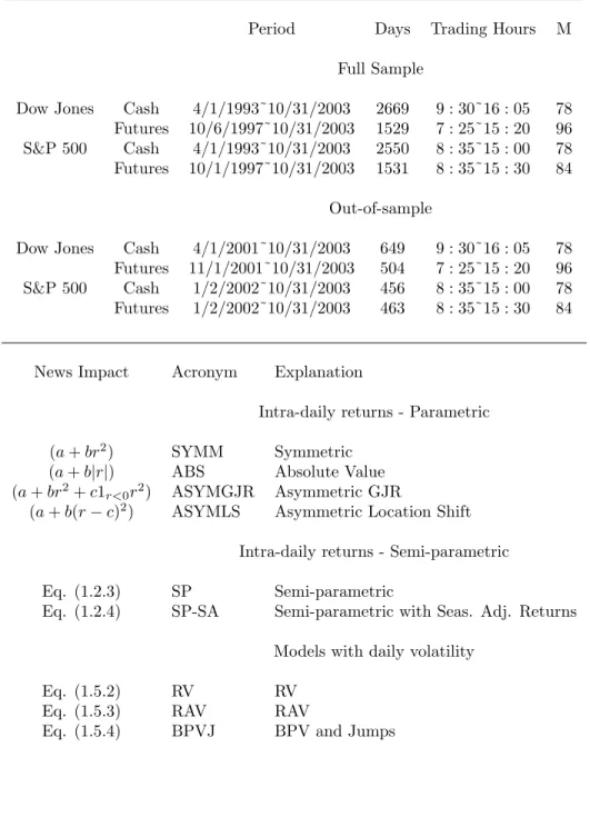
Table A.2 contains one day ahead forecasts for both parametric and semi-parametric model specifications, with acronyms provided in the lower panel of Table A.1. At this stage I have not yet discussed any of the parametric specifications, nor have I provided a rationale for them. This matter will be discussed later. For the moment, it is worth noting that the semi-parametric MIDAS regression models (denoted SP and SP-SA, the latter involving seasonally adjusted returns) provide the best out-of-sample fit for all the five-minute data (for each of the four series, the best models in terms of out-of-sample predictions appear as bold faced in Table A.2). It is also interesting to note that the semi-parametric models typically have the best in-sample fit. A comparison of SP and SP-SA indicates that using the raw five-minute data without adjustment is the best.

The parametric specifications include the RV, RAV and BPVJ models used

16 _{I construct the out-of-sample} _R2 _{as follows. I estimate the semi-parametric models over the} sample specified in Table A.1. Using data post-estimation sample I compute: R2_=1-_error2_/var₍_y₎ where error2 _{is the sum of squared difference between realized and predicted RV’s, and} _y _{is the} regressand.

17 _{Although the in-sample estimation results are similar for different number of grid points, the}

(29)

extensively in the current literature and based on aggregate daily volatility measures. It means that a regression model involving non-parametric estimation of a response function applied to high-frequency data, outperforms a fully parametric model involving daily aggregate measures such as RV, RAV and even the separation of jumps and continuous path volatility (identified via test statistics involving daily measures discussed in Andersen, Bollerslev, and Diebold (2006)). Typically, well specified

parametric models outperform semi-parametric ones. Here, however, the

semi-parametric models de facto use more data and are not subject to the pre-specified quadratic transformation of returns.

Since I have four volatility series, I consider four news impact curves in Figure A.1 at two horizons: one-day and one-week ahead. Unlike the plot appearing in the Introduction, I consider now four series instead of a single one. For the moment it suffices to look at the dotted lines in each of the figures, which represent the news impact curves obtained via the semi-parametric estimation. It is remarkable to note how similar the shapes are for the SP model across the four different series. For all series we recognize a similar shape. The asymmetry of the news impact is obvious. Negative and positive returns have a different impact. The finding that so called no news is good news extensively documented in the literature using daily returns has the minimum of the news impact curve at zero. Instead, with intra-daily data I find in Figure A.1 that the intra-daily news impact curves attain their minimum at some mildly positive return, meaning that such returns result in decreased volatility the next day (since the impact is negative).18 _{As noted in the Introduction, we also recognize the}

18_{The shape of the news impact curve should bring us back to the issue of positivity constraints. It}

(30)

fact that extremely ’good news’, the positive returns (it turns out those larger than the 90% quantiles), cause increased future volatility. Finally, as noted earlier, ’bad news’ has a more acute impact than positive news. To give specific numbers, for the DJ cash series the news impact curve achieves its minimum at 0.06 % five minute return and crosses into volatility increasing region at 0.12 % five minute returns. The other series yield similar results. It is also worth noting from the plots in Figure A.1 that the 95 % asymptotic confidence intervals around the news impact curves tell us that the dips below zero are statistically significant in all four cases.19

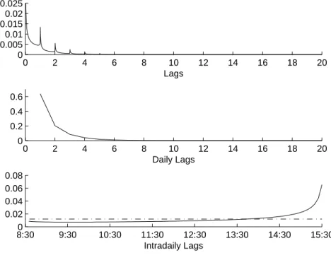
Besides the news impact curves, we need to discuss the parametric part of the semi-parametric MIDAS regression, or more specifically the Beta polynomials appearing in equation (1.2.5). I plot only one of the four examples, namely the S&P500 Futures example. There are three plots that appear in Figure A.2. The first plot displays the product of the daily and intra-daily lags, hence it contains the profile of the coefficients ψij. The second plot displays only the daily coefficients ψj and finally the intradaily coefficients ψi appears in the third plot. The patterns are not surprising, given the abundant evidence documented in the empirical volatility literature. The daily coefficients decrease monotonically and are close to zero after 6 to 8 days. The intra-daily weights display a somewhat asymmetric U-shaped pattern, perhaps best characterized as a smirk. It means that late afternoon returns, carry relatively more weight than morning returns. The product of the two provides a spiky decay pattern compounding the intra-daily and daily response.

Table A.2 also contains both parametric and semi-parametric model specifications

constraint mentioned earlier and also appearing in the Linton and Mammen code - was never binding.

19_{In the interest of space I do not report the curves involving the adjusted returns. It turns out that}

(31)

for the one-week and -month prediction horizon. Moreover, the plots appearing in

Figure A.1 also cover the weekly horizon news impact curves. We observe from

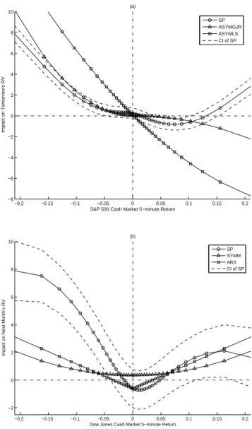
the patterns that as the horizon increases, the news impact curves tend to become symmetric and centered around the zero return axis. Hence, the same information set of five minute returns produces over longer horizons a more symmetric prediction pattern. This finding will clearly manifest itself later when I consider parametric models. The asymmetric ones will fare well at short horizons but not at longer horizons.

When we examine the results in Table A.2 we observe that the semi-parametric models hold up very well as far as forecasting out-of-sample goes. In fact the results in Table A.2 reveal that the semi-parametric MIDAS is the best across three out of four series for the monthly horizon. This is remarkable considering the fact that it is partially based on non-parametric estimation.

The empirical results also show a comparison of 5 minute, 10 minute and half-hourly sampled returns. With the semi-parametric MIDAS we note in general a decline in predictive power as we move to coarser sampling frequencies. This result is expected, as the 5 minute returns do not suffer from microstructure noise and aggregation of returns reduces the information content.

(32)

1.5 Parametric Models - New and Old

The findings discussed in the previous section wet our appetite for considering parametric models that apply directly to intra-daily data. There are at least three reasons for looking at a new class of parametric models. First, the models I will consider relate to GARCH-type models and hence bridge a new and old literature. Second, formal testing in the context of semi-parametric models is quite challenging while it is not in the case of parametric models. The most important and third reason is very practical. The estimation of semi-parametric MIDAS regressions is computationally demanding. The estimation time is roughly equal toMT ×τ M × n2

g whereMT is the sample size, τ M is the number of lags and ng is the number of grid points. Hence, in our examples with MT ' 200, 000,τ M ' 400 and ng = 41, estimation time is about 20 hours for PC with P4 2.4G CPU and 1GB Memory. In contrast, the parametric models introduced in this section take between 1 and 5 minutes to estimate with the same data.

The models I introduce are both old and new. They explore via parametric

(33)

adjusted returns, hence the classical debate about seasonal adjustment emerges here in the context of nonlinear time series regression models with mixed frequency data sampling. In a first subsection I introduce the new parametric models. The second subsection covers the empirical results.

1.5.1 A New Class of Parametric High Frequency Data

Models

The purpose is to introduce various parametric MIDAS regression models that are inspired by my previously introduced semi-parametric setup. To facilitate the presentation, I use the following indicator process: 1Awhich is one whenA is true, and equals zero otherwise. All models involving discretely sampled high frequency data can be represented in a generic parametric way:

RVt= τ

X

j=1

M

X

i=1

ψij(θ)NIC(rt−j−(i−1)/M) +εt (1.5.1)

wherePτ_j₌₁PM_i₌₁ψij = 1 and the following news impact curves (NIC) are used:

• NIC(r) = (a+br2_), _{to which I attach the acronym SYMM. The SYMM model}

can be regarded as a MIDAS extension of ARCH to the case of high-frequency data. Obviously, the SYMM model cannot capture any asymmetries that appear in the data. Note that the parameter a plays the role of the intercept in the regression equation (1.5.1), since the polynomial weights add up to one.

• Inspired by the GJR model proposed by Glosten, Jagannathan, and Runkle

(1993), I consider the ASYMGJR model with NIC(r) = (a +br2 ₊_c1

r<0r2).

(34)

data. So, the constraint is not imposed in the ASYMGJR model.

• Another possible way to allow for asymmetric effects is via a location shift, as in the Asymmetric GARCH model in Engle (1990b), yielding the ASYMLS model with NIC(r) = (a+b(r−c)2_).20

• The last model with the intra-daily return considered in my study is the ABS model withNIC(r) = (a+b|r|), which is again a symmetric model. It relates to the use of RAV (Realized Absolute Value) as a regressor on a daily basis.

All of the above models are compared to the more traditional daily volatility models. I consider three cases of regressors: RV, RAV, BPV and Jumps yielding the RV model, RAV model and BPVJ model, respectively. All these models are in the framework of MIDAS regression, namely:

RVt=a+b τ

X

j=1

ψj(θ)RVt−j +εt (1.5.2)

RVt=a+b τ

X

j=1

ψj(θ)RAVt−j+εt (1.5.3)

RVt=a+b τ

X

j=1

ψj(θ)BP Vt−j + 1jump,t−1(c+d(RVt−1−BP Vt−1)) +εt (1.5.4)

where ψj(θ) = Beta(j, τ, θ1, θ2); 1jump,t−1 indicates if there is jump at day t−1 and

RVt−1 −BP Vt−1 is the size of the jump at day t−1. We use the test suggested by

Huang and Tauchen (2005) to determine 1jump,t.

20_{I also considered two models which combine the GRJ model and Asymmetric GARCH model:}

ASYMC1 model,N IC(r) = (a+b1r−d<0(r−d)2+c1r−d≥0(r−d)2); and ASYMC2 model,N IC(r;θ)

= (a+b1r<0(r−d−e)2+c1r≥0(r−d)2). I do not report the results as they were roughly similar to

(35)

1.5.2 Empirical Results

The full-sample estimation and out-of-sample forecasts are shown in Tables A.2, again for one-day, one-week and one-month horizons. I cover first the one-day ahead horizon. According to the R2_{s in the full-sample, the parametric models (using unadjusted}

returns) can be divided into two groups: the first group consists of the asymmetric ASYMGJR and ASYMLS models; the second group consists of the rest - i.e. the symmetric ones. Again, for the one-day horizon, the R2_{s of the models in the first}

group is in general 5% to 7% greater than those in the second group. The in-sample results also hold in the out-of-sample forecasts comparisons. Hence, the asymmetric effect is an important feature of the news impact curve in the high-frequency data case. It is also worth noting that symmetric models using intra-daily data still typically outperform the traditional models based on daily volatility measures, i.e. the RV, RAV and BPVJ models. Hence, the information gain from intra-daily squared or absolute returns is genuine and the superior forecasting performance is not entirely due to the functional mis-specification of asymmetric effects. Yet, the bulk of the gains are due to mis-specification. Comparing the SYMM and ABS high frequency data models with RV and RAV, we note that the out-of-sample forecasting improvements are small, whereas the asymmetric models are far superior to RV and RAV.

Tables A.2 also contain parametric models with seasonally adjusted returns, using the three different sampling frequencies. Comparing models involving seasonally adjusted versus unadjusted returns I find that it is fairly even in terms of out-of-sample prediction performance without a clear pattern. However, in all cases, the difference between a model with and without adjustment is typically small.

(36)

symmetric, as noted from the semi-parametric estimates in Figure A.1. The news impact curves of two asymmetric models at the one-day horizon, the ASYMLS and ASYMGJR models, are shown in Figure A.3 (top panel - S&P 500 cash series). Comparing the news impact curves of the SP model with the two asymmetric parametric models, we find that the ASYMGJR and SP curves are very similar for negative returns. However, for extremely good news the two diverge. In contrast, the ASYMLS model is not of the same shape, yet it does better than the ASYMGJR model in terms of out-of-sample forecasting. The plot shows that the parametric models still do not fully capture the news impact as recovered via semi-parametric estimation, and also explains why the latter features superior forecasting performance. The same goes through for the one-month horizon symmetric parametric models, as Figure A.3 (lower panel - DJ cash series) indicates.

To conclude the discussion of empirical results we turn our attention to Table A.3. For a selection of models and horizons, I report the empirical estimates of the parametric models. It appears from the results in the table that parameter estimates of the asymmetric effect (i.e. the parameter c) appears significant, even at the weekly forecast horizon.21

The overall picture that emerges can be summarized as follows. I essentially made three types of forecasting performance comparisons. They are (1) semi-parametric with parametric models - both using high frequency data, (2) parametric models that use aggregate measuresRV, RAV,andBP V J - all three being implicitly symmetric- with parametric models using high frequency data directly that are also symmetric, and (3) parametric models that use high frequency data and are asymmetric with parametric models also using high frequency data directly but are symmetric. The comparison in (3) deals with parametric mis-specification, i.e. the role played by asymmetry. The

(37)

comparison (2) tells us something about loss of information due to aggregation and finally (1) reveals mis-specification of the parametric models. My empirical findings show that the forecasting gains are mostly due to asymmetries, and the parametric models I consider still do not fully capture all asymmetries - which is why the semi-parametric MIDAS regressions outperform all other approaches.

1.6 Conclusions

I introduce semi-parametric MIDAS regressions and study their large sample behavior. While semi-parametric MIDAS regressions potentially apply in a variety of settings, the main focus of this chapter is on a specific application, namely news impact curves. The regression models also inspired a new class of parametric volatility models that apply directly to high-frequency data. The writing of Engle and Ng (1993) was in part motivated by the recognition that volatility models, including the at time very popular daily GARCH(1,1) model of Bollerslev (1986), imposed a particular response function of shocks to volatility and that most often such response functions were inherently misspecified. The most preferred model of Engle and Ng (1993), based on their empirical analysis, was that of Glosten, Jagannathan, and Runkle (1993). The main findings of this literature still remain very much part of our core beliefs today regarding the key stylized facts of volatility dynamics. Namely, it is widely believed that

(38)

impact. The asymmetry evaporates at longer horizons. Parametric specifications, which bridge the new and old literature, confirm these findings of asymmetry at short and longer horizons via simple hypotheses imposed on the parameters.

(39)

Chapter 2 News is more than one dimensional

2.1 Introduction

It is difficult to define ’news’. Most academic papers look at a single series, say the market return, and measure the impact of unexpected events - typically a prediction error - onto future outcomes such as future volatility. In practice, market participants absorb news from many sources simultaneously. It is the purpose of this chapter to try to capture this multi-dimensional aspect of news, with as a specific example the impact of market-wide and firm-specific news on the future volatility of individual firms.

The topic of this chapter obviously relates to multivariate volatility models and more specifically the notion of news impact curve, due to Engle and Ng (1993), and its multivariate extensions. Multivariate ARCH-type models, such as the VEC model of Bollerslev, Engle, and Wooldridge (1988), the BEKK model of Engle and Kroner (1995), the CCC model of Bollerslev (1990), the DCC model of Engle (2002), and GDC model of Kroner and Ng (1998) implicitly deal with the impact of news on future volatility.1 _{However, in multivariate ARCH-type models, the sources of news is usually}

equal to the number of assets considered.

(40)

In this chapter I adopt a framework where possibly a single asset is considered -say an individual firm - affected by multiple sources of news. Chapter 1 defines news as a return over a very short time interval and then measure its impact over multiple horizons. The method is applied only in a univariate setting. I extend the method of Chapter 1 to the case of multi-dimensional news and define news as the high-frequency returns, e.g., 30-minute returns in this chapter, of the individual stocks and the market index.2

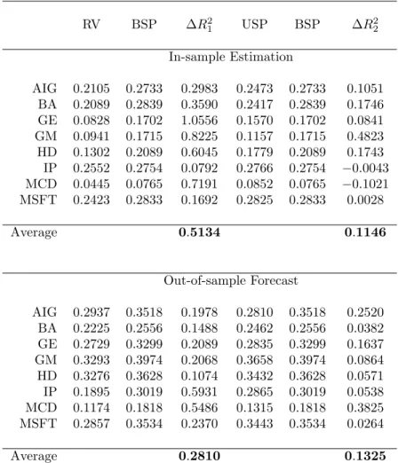
The high-frequency returns of the market index, e.g., S&P 500 index in this chpater, represent the market-wide news. However, the returns of an individual stock not only contains firm-specific news, but also the market-wide news. It is therefore necessary to separate, in this case, the two sources of news. To do so, I use the concept of news impact surface, which was established by Kroner and Ng (1998) as an extension of the concept of news impact curve by Engle and Ng (1993). Unlike the ARCH-type parametric setting, I use a semi-parametric setup. This is appealing as it might be better at capturing the complexity of the various sources of news, despite the potential problems associated with ”curse-of-dimensionality”. Indeed, the empirical results show that the multivariate extension of semi-parametric MIDAS models is a good tool to measure the impact of high-dimensional news. I also build various new parametric models based on two-dimensional news. As a comparison, some models based on one-dimensional news are estimated. I find that (1) the models based on multi-one-dimensional news show better in-sample fit and out-of-sample forecast performance than the models based on one-dimensional news; (2) in the case of multi-dimensional news, there still exists the asymmetric effect of news, i.e., good news and bad news with the same magnitude have a different effect on the future volatility; (3) The impacts on volatility

2_{Sampling frequencies other than 30 minutes interval are a possibility. I select this specific frequency}

(41)

by two sources of news are interactive and firm specific.

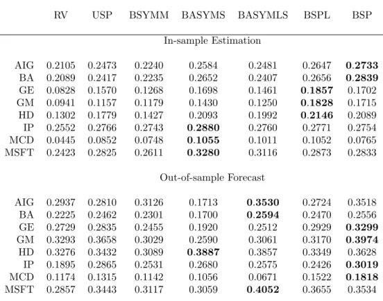
The chapter is organized as follows. In section 2.2, I construct various of bivariate parametric and semi-parametric models in the framework of MIxed DAta Sampling (henceforth MIDAS) regressions, followed in section 2.3 by the estimation method and asymptotic properties of the generic multivariate semi-parametric MIDAS models. The empirical study is shown in section 2.4. Finally, section 2.5 concludes the chapter and points out some directions of the future work.

2.2 Bivariate

Parametric

and

Semi-parametric

Models

The purpose of this section is to introduce the parametric and semi-parametric models. I first discuss how to separate market-wide news and firm-specific news. Then, a new class of parametric models and a semi-parametric model based on two sources of news will be proposed, followed by a more general semi-parametric model. Finally, two univariate models will be listed as a comparison.

To set forth notation, let the unit interval correspond to one day. The high-frequency returns are sampled at the frequency M, i.e., the discretely observed compounded returns of the individual stock and the market index can be recorded as{r_s/M(i) , r(_s/Mm)}s≥0.

Obviously, rs/M is the kth intra-daily return at day t, where s = (t −1)∗ M + k and 1 ≤ k ≤ M, so sometimes I use the notation rt+k/M instead of rs/M. The Realized Volatility at dayt,RVt, which is the practical implementation of the integrated volatility, is defined as follows:

RVt= M

X

k=1

(42)

As indicated in the Introduction, the high-frequency return of the individual stock r(i) _{contains two types of news: market-wide news and firm-specific news. Since the}

market-wide news can be measured by the high-frequency return of the market index r(m)_{, the question remaining is how to extract the firm-specific news, denoted by} _r(f)_,

from the return of the individual stock. In the simplest case, let’s assume that the two types of news is linearly combined in the individual stock return, i.e., the relationship can be expressed in the following equation:

r_s/M(i) =βr_s/M(m) +r_s/M(f) (2.2.2)

Hence, rearranging equation (2.2.2), we can obtain the firm-specific news:

r_s/M(f) =r_s/M(i) −βr_s/M(m) (2.2.3)

It is the well-known way to define market beta in the Capital Asset Pricing Model

(CAPM).3

All our models to be proposed are in the framework of the MIxed DAta Sampling, MIDAS, regressions, which deal with data sampled at different frequencies. MIDAS regressions have been widely applied in the context of volatility forecasting by Forsberg and Ghysels (2006), Ghysels, Santa-Clara, and Valkanov (2006), Ghysels, Sinko, and Valkanov (2006), among others. To predict the volatility with the high-frequency return, I propose the following generic MIDAS regression model:

RVt= τ

X

j=1

M

X

k=1

ψkj(θ)NIS(r_t−j(f)₊₍_k−₁₎_/M, r_t−j(m)₊₍_k−₁₎_/M) +εt (2.2.4)

(43)

where ψkj(θ) is a known lag coefficients function of the unknown parameters θ = (θ1, θ2, θ3, θ4) and NIS(., .) is a function representing the impact on the future

volatility by the two sources of news. The parametric specification I consider will be multiplicative for intra-daily/daily lags, the same as that in Chapter 1 to deal with the seasonality in high-frequency returns. Namely, I define ψkj(.) as:

ψkj(θ) = ψj(θ)ψk(θ) =Beta(j, τ, θ1, θ2)×Beta(k, M, θ3, θ4) (2.2.5)

whereBeta(l, L, α, β) = (l/(L+1))α−1₍₁₋_l/(L+1))β−1_{Γ(α+β)/Γ(α)/Γ(β) and Γ(α) =}

R₊_∞

0 e−ttα−1dt. Intra-daily patterns are accommodated via Beta(k, M, θ3, θ4) while the

daily memory decay is patterned viaBeta(j, τ, θ1, θ2). Note that I impose the restriction

that the intra-daily patterns wash out across the entire day, i.e. I impose the restriction that the weights of the intra-daily polynomial add up to one,P_kBeta(k, M, θ3, θ4) = 1.

I could also impose a similar restriction on the daily polynomial in order to separately identify a slope coefficient.

The remaining problem is to determine the form ofNIS(., .). I consider four kinds of functionals:

1. BSYMM model:

NIS(r(f), r(m)) = α0+α1(r(f))2+α2(r(m))2+α3r(f)r(m) (2.2.6)

(44)

2. BASYMS model:

NIS(r(f)_{, r}(m)_{) =} _α

0+α1(r(f))2+α2(r(m))2+α3r(f)r(m) (2.2.7)

+α41r(f)_<₀(r(f))2+α₅1_r(m)_<₀(r(m))2+α₆1_r(f)_<₀1_r(m)_<₀r(f)r(m)

+α71r(f)_≥₀1_r(m)_<₀r(f)r(m)+α₈1_r(f)_<₀1_r(m)_≥₀r(f)r(m)

The BASYMS model is inspired by the GJR model proposed by Glosten, Jagannathan, and Runkle (1993), who consider the effect of the sign of the news.

3. BASYMLS model:

NIS(r(f)_{, r}(m)_{) =}_α

0+α1(r(f)−α4)2+α2(r(m)−α5)2+α3(r(f)−α4)(r(m)−α5)

(2.2.8) The BASYMLS model shows another possible way to allow asymmetric effects: with location shifted. It is inspired by the asymmetric GARCH model of Engle (1990a).

4. BSPL model:

NIS(r(f)_{, r}(m)_{) =}_n(r(f)_{, r}(m)₎ _(2.2.9)

The BSPL model is a bivariate semi-parametric MIDAS model. Here, n(., .) is a unknown non-parametric function. It is flexible and avoids the misspecification error. The estimation result can be interpreted through the news impact surface. Note that the last letter in the acronym BSPL stands forlinearbecause this model depends on the assumption that the firm-specific news can be extracted through the linear regression (2.2.3). How to estimate this model will be discussed in the next section.

(45)

forecast ability of the model. I propose the following bivariate semi-parametric MIDAS regression model, BSP model, to relax the linear assumption:

RVt = τ

X

j=1

M

X

k=1

ψkj(θ)m(r_t−j(i) ₊₍_k−₁₎_/M, r_t−j(m)₊₍_k−₁₎_/M) +εt (2.2.10)

In fact, the non-parametric function n(., .) in BSPL model should be equivalent to m(., .) since n(r(f)_{, r}(m)_{) =}_n(r(i)₋_βr(m)_{, r}(m)_{) =}_m(r(i)_{, r}(m)_{). It is expected that the}

BSPL model has the similar in-sample estimation as the BSP model, which is confirmed by the empirical study. However, the linear transformation requires the estimated β. If the linear assumption is wrong, the out-of-sample forecast performance of the BSPL model may be worse than that of BSP model, which is also confirmed by the empirical evidence.

As a comparison, I consider the RV model and the univariate semi-parametric MIDAS models considered in Chapter 1. The definition of the RV model is as follows:

RVt = τ

X

j=1

ψj(θ)(γ0+γ1RVt−j) +εt (2.2.11)

where ψj(θ) = Beta(j, τ, θ1, θ2). The definition of the Univariate Semi-Parametric

MIDAS (USP) model is as follows:

RVt= τ

X

j=1

M

X

k=1

ψkj(θ)m(r(_t−ji)₊₍_k−₁₎_/M) +εt (2.2.12)

(46)

2.3 Multivariate

Semi-parametric

MIDAS

Regression Models

One of the novel features introduced in this paper is the multivariate semi-parametric

MIDAS regression model. It can be regarded as an extension of the univariate

semi-parametric MIDAS models introduced in Chapter 1. In this section, a generic specification is first introduced. Then, the estimation method and asymptotic properties are discussed.

2.3.1 Model specification and Estimation Method

As a starting point, it is worth recalling that our estimation is mainly inspired by the method proposed by Linton and Mammen (2005). They use kernel smoothing methods and solve a so called type II linear integration equation to estimate the semi-parametric ARCH(∞) model, which is expressed via the following equation:

σ_t2 = ∞

X

j=1

ψj(θ)m(rt−j) (2.3.1)

where rt are daily returns; σt2 is the conditional variance of the return; ψj(.) is a known function, e.g., ψj(θ) = θj−1_{; hence} _θ _{is an unknown parameter and} _{m(.) is an}

unknown function. Chapter 1 adopts their method and extend it to the univariate semi-parametric MIDAS model. In this section, I will further extend the estimation method to the multivariate case. I discuss the semi-parametric model estimation in a generic setting:

yt= τ

X

j=1

Bj(θ)m(xt−1−(j−1)/M) +εt (2.3.2)

The semi-parametric midas models and some of their applications : the impact of news on the stock volatility