Indirect Inference Estimation of Mixed
Frequency Stochastic Volatility State Space
Models using MIDAS Regressions and
ARCH Models
P. Gagliardini
1, E. Ghysels
2and M. Rubin
31Universita della Svizzera Italiana and Swiss Finance Institute,2University of North Carolina— Chapel Hill and3University of Bristol
Address correspondence to E. Ghysels, University of North Carolina - Chapel Hill, Gardner Hall, CB 3305 Chapel Hill, NC 27599-3305, or e-mail: [email protected].
Received December 3, 2016; revised December 3, 2016; editorial decision December 7, 2016; accepted January 14, 2017
Abstract
We examine the relationship between Mixed Data Sampling (MIDAS) regressions and the estimation of state space models applied to mixed frequency data. While in some cases the binding function is known, in general it is not, and therefore indirect infer-ence is called for. The approach is appealing when we consider state space models which feature stochastic volatility (SV), or other non-Gaussian and nonlinear settings where Maximum Likelihood (ML) methods require computationally demanding ap-proximate filters. The SV feature is particularly relevant when considering high fre-quency financial series. In addition, we propose a filtering scheme which relies on a combination of reprojection methods and nowcasting MIDAS regressions with ARCH models. We assess the efficiency of our indirect inference estimator for the SV model by comparing it with the ML estimator in Monte Carlo simulation experiments. The ML estimate is computed with a simulation-based Expectation-Maximization (EM) al-gorithm, in which the smoothing distribution required in the E step is obtained via a particle forward-filtering/backward-smoothing algorithm. Our Monte Carlo simula-tions show that the Indirect Inference procedure is very appealing, as its statistical ac-curacy is close to that of MLE but the former procedure has clear advantages in terms of computational efficiency. An application to forecasting quarterly GDP growth in the Euro area with monthly macroeconomic indicators illustrates the usefulness of our procedure in empirical analysis.
Key words: GDP forecasting, indirect inference, MIDAS regressions, state space model, stochas-tic volatility
JEL classification: C15, C32, E37
VCThe Author, 2017. Published by Oxford University Press. All rights reserved. For Permissions, please email: [email protected]
Econometric models that take into account the unbalanced nature of datasets have attracted substantial attention recently. Policy makers and practitioners alike need to assess in real time the current state of the economy, with at best mixed frequency data at their dis-posal. For example, one of the key indicators of macroeconomic activity, the Gross Domestic Product (GDP), is released quarterly, while a range of leading and coincident indicators is timely available at a monthly or even higher frequency. Hence, we may want to construct a forecast of the current quarter GDP growth (a so-called nowcast) based on the available higher frequency information.
Econometric models with mixed frequency data can be classified into two broad classes: (i) likelihood-based involving latent processes and (ii) purely regression-based. The former category consists primarily of state space models, studied by Harvey and Pierse (1984),
Harvey (1989),Zadrozny (1990),Bernanke, Gertler, and Watson (1997),Mariano and
Murasawa (2003),Mittnik and Zadrozny (2005), Aruoba, Diebold, and Scotti (2009),
Ghysels and Wright (2009),Kuzin, Marcellino, and Schumacher (2011), among others.
The regression-based methods involve Mixed Data Sampling (MIDAS) regressions; see for example Ghysels, Santa-Clara, and Valkanov (2006),Andreou, Ghysels, and Kourtellos (2010). As one considers high frequency (HF) data, the issue of time-varying volatility becomes increasingly relevant. Dealing with stochastic volatility (SV) in state space models is doable but poses challenges both statistical and computational in nature. One possibility is to consider Bayesian approaches in this context, as done by Carriero, Clark, and
Marcellino (2013) and Marcellino, Porqueddu, and Venditti (2016). However, when it
comes to classical inference one typically relies on the Expectation-Maximization (EM) algorithm to compute numerically the ML estimate in a model with unobservable variables (Dempster, Laird, and Rubin, 1977). The likelihood function of the model involves a large-dimensional integral with respect to the latent factor paths as the latent factors appear in the conditional mean and volatility of the HF data series. This integral representation of the likelihood is impractical for the computation of the ML estimate.
If the objective is to estimate state space models with mixed frequency data—of which there are many examples—featuring SV, using classical inference methods, is there perhaps a simpler way to do so? This is the contribution of our article. We introduce indirect infer-ence estimation procedures proposed byGourie´roux, Monfort, and Renault (1993),Smith (1993)andGallant and Tauchen (1996), to estimate the models of interest using MIDAS regressions augmented with ARCH-type models as well as mixed frequency Vector Autoregressive (VAR) models (see e.g.Ghysels (2016)) as auxiliary models. Same frequency data settings are a special case of mixed frequency ones. The analysis in this article is there-fore also applicable to standard state space models. Moreover, the idea of estimating SV-type models using ARCH-SV-type auxiliary models has a long history starting withEngle and Lee (1999)andPastorello, Renault, and Touzi (2000). Our article combines insights from the literature on SV models with those from the mixed frequency data literature.
addition, we filter latent variables, given observables, using reprojection methods proposed byGallant and Tauchen (1998).
We compare the two estimation methods, namely (i) Maximum Likelihood (ML) and (ii) indirect inference, via Monte Carlo simulations. To implement the former method in the mixed frequency SV model, we consider a simulation-based estimator relying on the EM algorithm. The smoothing distribution required in the Expectation step is computed via a particle forward-filtering/backward-smoothing algorithm. We compare the two esti-mation methods on the basis of (i) statistical criteria—mean/bias/quantiles of sampling dis-tributions, (ii) filtering accuracy—both conditional mean and volatility, and (iii) computational time. Our results show that there are clear advantages in terms of computa-tional time to the new indirect inference procedure put forward in this article, while the losses in statistical efficiency compared to MLE are very limited. Even in the linear Gaussian case, we find our indirect inference methods remarkably accurate, when com-pared to the standard Maximum Likelihood Estimation (MLE) based on the Kalman filter.
The article is organized as follows. Section 1 introduces state space models with mixed frequency data and SV. Section 2 defines our indirect inference estimator. This section cov-ers the linear Gaussian state space model with mixed frequency data as a special case of the general specification, and discusses its relation with MIDAS regressions. This link yields useful insights to define the auxiliary model for indirect inference in the general SV case. Section 2 also describes the estimation of the SV model with ML via a simulation-based EM algorithm. Section 3 discusses filtering via reprojection, followed by Section 4 which reports the results of an extensive Monte Carlo study. Section 5 presents an empirical appli-cation of our model to the problem of forecasting at short horizons Euro-area quarterly GDP growth using monthly macroeconomic indicators. The dataset is the same as the one considered in the empirical study ofMarcellino, Porqueddu, and Venditti (2016). Section 7 concludes the article.
1 State Space Models with Mixed Frequency Data and SV
There is a burgeoning literature on nowcasting using either MIDAS regressions or state space models, see for exampleMariano and Murasawa (2003),Nunes (2005),Giannone,
Reichlin, and Small (2008), Aruoba, Diebold, and Scotti (2009), Marcellino and
Schumacher (2010),Andreou, Ghysels, and Kourtellos (2013)andBanbura and Modugno
(2014), among others. Recent surveys includeAndreou, Ghysels, and Kourtellos (2011), Foroni and Marcellino (2015)andBanbura et al. (2013), where the latter paper has a stron-ger focus on more complex Kalman filter-based factor modeling techniques.
State space models have been widely used in econometrics as well as other scientific dis-ciplines, in particular engineering where the Gaussian state space model and its Kalman fil-tering algorithm originated.1A key starting point is that observations are driven by some
latent process. Moreover, it is also assumed that data are contaminated by measurement errors. To accommodate the mixed frequency sampling scheme, we adopt a time scale expressed in a form that easily represents such mixtures. We will focus on small values of
m, the number of HF subperiods, such as for examplem¼3 for monthly data sampled every quarter. We consider a dynamic model for the latent factors as follows:
Assumption 1.1. Let (F) be a nf1dimensional vector process satisfying
Ftþj=m¼
Xp
l¼1
UlFtþðjlÞ=mþgtþj=m 8t¼1;. . .;T; j¼0;. . .;m1; (1.1)
whereUlare nfnf matrices, the eigenvalues of the autoregressive matrix in the stacked
AR(1) representation lie inside the unit circle, andð Þg is an i.i.d. zero mean Gaussian error
process with diagonal covariance matrixRg¼diag(r2i;g;i¼1;. . .;nf). Finally, the number
of factors nf;is assumed to be known.
We have two types of data: (i) time series sampled at a low frequency (LF)—every inte-ger datet, and (ii) time series sampled at HF—everytþj/m, withj¼0;. . .;m1.Bai, Ghysels, and Wright (2013)make two convenient simplifications which depart from gener-ality. First, they assume that there is only one LF process and call ityt;and second, consider
the combination of only two sampling frequencies. We will proceed with the same simplifi-cations and also assume—for the sake of simplicity—that there is only one HF series, denoted xtþj=m: It is fairly easy to extend the methods proposed in this article to cases
involving multiple LF and HF series—which we will not cover explicitly.
If the LF process were observed at HF, it would relate to the factors as follows:
y
tþj=m¼c01Ftþj=mþu1;tþj=m 8t; j¼0;. . .;m1; (1.2)
whereydenotes the process which is not directly observed andc
1is anf1 vector of
fac-tor loadings. The error processu1;tþj=mhas anAR(k) representation:
d1 L1=m
u1;tþj=m¼e1;tþj=m; d1 L1=m
1d11L1=m. . .dk1Lk=m; (1.3)
where the lag operatorL1=mapplies to HF data, that isL1=mu
tut1=m:The observed LF
processyrelates to the processyvia a linear aggregation scheme:
yc
tþj=m¼Wjyctþðj1Þ=mþkjytþj=m (1.4)
whereytis equal to the cumulator variableyct for integert, and is not observed otherwise.
The above scheme, also used byHarvey (1989)andNunes (2005), covers both stock and flow aggregation. We get the case of a stock variable by settingWj¼1ðj6¼0;m;2m:::Þand
kj¼1ðj¼0;m;2m; :::Þ, where 1ð Þ: denotes the indicator function. If we pick instead
Wj¼1ðj6¼1;mþ1;2mþ1; :::Þandkj¼1=mfor allj, then we get a flow variable.
The HF processxtþj=mrelates to the factors as follows:
xtþj=m¼c20Ftþj=mþu2;tþj=m 8t; j¼0;. . .;m1; (1.5)
wherec2is anf1 vector and:
d2 L1=m
u2;tþj=m¼e2;tþj=m; d2 L1=m
1d12L1=m. . .dk2Lk=m: (1.6)
As usual in latent factor models, factor loadings c1,c2and the parameters of the factor
The standard approach is to assume that the innovation processesð Þek are i.i.d. Gaussian
with mean zero and variancer2
ek, fork¼1, 2. Indeed, the literature typically ignores the pres-ence of time-varying volatility, yet the HF data often involve financial and other series which feature conditional heteroskedasticity. This means that the state space models are no longer Gaussian. There is a substantial literature on non-Gaussian state space models tailored for the analysis of financial returns data (see e.g.Ghysels, Harvey, and Renault (1996),Shephard (2005)and references therein). The type of models of interest to us are rather state space models with SV in measurement equations. Hence, our analysis relates more directly to recent work by Clark (2011), Carriero, Clark, and Marcellino (2012), Carriero, Clark, and Marcellino (2013), orMarcellino, Porqueddu, and Venditti (2016).
We augment Equations (1.5)–(1.6) for HF data with time-varying volatility:
e2;tþj=m N0;htþj=m; (1.7)
where the log volatility follows a Gaussian autoregressive process:
lnhtþj=m¼cþqSVlnhtþðj1Þ=mþntþj=m; ntþj=mi:i:N 0; 22
; (1.8)
and parameterqSVis smaller than 1 in absolute value. We obtain a SV-type volatility
speci-fication without common factor structure.
While our analysis relates to recent work by Marcellino, Porqueddu, and Venditti (2016), among others, as noted before, there are also subtle but important differences. In their model, the factor process features SV. Instead, inEquation (1.7)we assume that the measurement error features SV. When dealing with LF macroeconomic series exposed to factors, we think it is more appropriate to assume that those factors do not feature volatility clustering, while the HF series are conditionally heteroskedastic. Ideally one could consider models where SV is featured in both the observation and state equations. This is of course a model choice decision. SV or ARCH features, while prominently present in HF series, are diminished in importance when it comes to LF phenomena. Temporal aggregation is one argument. For our analysis, the factor tracks LF data, and retrieves that information from HF data as well—albeit contaminated with noise that indeed features volatility clustering. We leave this as a topic for future research. Assumptions 1.1 and 1.2 (below) define the parametric models of interest in this article. We denote byhthe vector of unknown parame-ters in these models.
Assumption 1.2. The observable processes (y) and (x) are such that:
y
tþj=m¼c01Ftþj=mþu1;tþj=m;
d1L1=mu1;tþj=m¼e1;tþj=m; d1L1=m1d11L1=m. . .dk1Lk=m;
yc
tþj=m¼Wjyctþðj1Þ=mþkjytþj=m;
yt¼yct;
xtþj=m¼c02Ftþj=mþu2;tþj=m;
d2 L1=m
u2;tþj=m¼h1tþ=2j=me2;tþj=m; d2 L1=m
1d12L1=m. . .dk2Lk=m;
wherejqSVj < 1, andð Þe1 ;ð Þe2 ;ð Þn are mutually independent i.i.d. Gaussian processes, with
distributionsN 0;r2
e1
;Nð0;1Þ;N 0; 2 2
respectively, and independent of processð Þg.
2 Indirect Inference Estimation
Estimating via ML the mixed frequency models with SV presented in the previous section is rather involved. Indeed, the likelihood function involves a large-dimensional integral with respect to the latent factors path. This integral representation of the likelihood is impracti-cal for computation of the ML estimate, and numeriimpracti-cal filtering techniques are necessary.
In this section, we introduce indirect inference estimation methods—proposed by Gourie´roux, Monfort, and Renault (1993),Smith (1993)andGallant and Tauchen (1996)— to estimate the mixed frequency SV models. Indirect inference can be used to estimate virtu-ally any model from which it is possible to simulate data. This obviously includes state space models. Indirect inference estimation in fact involves two types of models—a model of inter-est already specified in the previous section—and an auxiliary model which is easy to inter- esti-mate. Both models are linked—in terms of parameter spaces—by a binding function.
2.1 Linear Setting with Known Binding Function
To explain our estimation approach, it is worth starting with a setting where the binding function is known. This setting is provided by a linear state space model with Gaussian errors. This model is a special case of the general specification in Assumptions 1.1 and 1.2 when there is no SV.2In this linear state space model, the Kalman filter can be applied for
prediction and filtering.Bai, Ghysels, and Wright (2013)show that for a model with a single latent factor (nf¼1) having a AR(1) dynamics and persistence parameterq, andm¼3 as for
instance for a monthly/quarterly mixture of data, one obtains (see Appendix A.2 for details):
E ytþhjItM
¼q3hj3;1 X1
j¼0
#jytjþq3h X1
j¼0
#jxð Þhxtj; (2.1)
where IM
t denotes the information in the available LF and HF data up to time t,
#¼½ðqqj1Þðqqj2Þðqqj3Þ, and ji, j3;i are steady state Kalman gain parameters.
Moreover, one has:
xð Þhx t j3;2þðqqj3Þj2L1=3þðqqj3Þðqqj2Þj1L2=3
h i
xt (2.2)
which is a parameter-driven LF process composed of HF data aggregated at the quarterly level.
The above equation relates to the multiplicative MIDAS regression models considered by Chen and Ghysels (2010)andAndreou, Ghysels, and Kourtellos (2013). In particular consider the following ADL-MIDAS regression:
ytþh¼by
XKy
j¼0
wj hy ytjþbx
XKx
j¼0
wj h1x
j
xh2x tjþetþh; (2.3)
wherewj hy ;wj h1x follow an exponential Almon scheme and
x h2x tjX
m1
k¼0
wk h2x Lk=mxtk=m
also follows an exponential Almon scheme.3Provided that
q>0,Equation (2.1)is a spe-cial case of this model withKy¼Kx¼ 1;wj hy /exp logð ð Þ# jÞ;wj h1x /exp logð ð Þ#jÞ
and wk h2x /exp h2x;1kþh2x;2k2
where h2x;1 and h2x;2 are parameters that solve the
equations:
logðqqj3Þj2=j3;2 ¼h2x;1þh 2
x;2;
logðqqj3Þðqqj2Þj1=j3;2 ¼2h2x;1þ4h 2
x;2:
(2.4)
Equations (2.3)and (2.4) implicitly define a binding function between the parameters of the state space model and those of the MIDAS regression. Note, however, that the mapping under-identifies the parameters of the state space model if we rely on a standard multiplica-tive MIDAS regression scheme. Moreover, the mapping is only valid for a single factor state space model with i.i.d. measurement errors. What do we do for multifactor models or single factor models with autoregressive errors? Bai, Ghysels, and Wright (2013) show that MIDAS regressions still provide very accurate approximations, although there is no exact (underidentified) mapping.
2.2 Auxiliary Models: U-MIDAS and ARCH
A departure from the setup inBai, Ghysels, and Wright (2013)is that we replaceEquation
(2.3)with a U-MIDAS—meaning unrestricted MIDAS—specification suggested byForoni,
Marcellino, and Schumacher (2015), namely:
ytþ1¼b0þ
XK~y
k¼0
bkytkþ X mðK~xþ1Þ1
j¼1
cjxtþ1j=mþetþ1: (2.5)
Note that we estimateK~yþmK~xþ1parameters (not including intercept and residual
variance). Whenmis small, as shown byForoni, Marcellino, and Schumacher (2015), we are able to estimate these parameters with reasonable precision using sample sizes typi-cally encountered in economic applications. One attractive feature of U-MIDAS misspeci-fication is the fact that estimation is numerically straightforward, as it can be performed by OLS.
Suppose we collect all the parameters of the U-MIDAS regression into the vector/2U:
Assuming dimð Þ h dimð Þ / K~yþmK~xþ1þ2 we may be able to identify and estimate
the parameters via indirect inference.4
3 The constructed LF regressor is estimated jointly with the other (MIDAS) regression parameters. Hence, one can viewx h2
x tj as the bestaggregatorthat yields the bestprediction.This ADL-MIDAS regression involves more parameters than the usual specification involving only one polynomial.
Since the models of interest feature SV, we can consider as auxiliary models the follow-ing U-MIDAS regressions augmented with ARCH errors:
ytþ1¼b0þ
XK~y
k¼0
bkytkþ X mðK~xþ1Þ1
j¼1
cjxtþ1j=mþetþ1; etþ1 N 0;r2tþ1
r2
t ¼xþ Xp
k¼1
ake2tk
(2.6)
which has the advantage of being simple to implement as it only involves a linear regression specification with ARCH(p) errors. The idea for this auxiliary model is that heteroskedas-ticity in the HF data affects the residuals of the reduced form MIDAS regressions. Obviously, the ARCH model in the above equation is only estimated at LF, and therefore the ARCH effects may not be particularly strong.
2.3 Auxiliary Models: Mixed Frequency VAR and ARCH
The auxiliary U-MIDAS regressions considered in the previous subsection do not fully exploit all features of the data since the link between latent factors and HF data is not being taken into account. In this subsection, we remedy to this shortcoming by considering mixed frequency VAR models. It is worth noting from the start that there might be some confu-sion about the characterization of mixed frequency VAR models. The analysis below serves two purposes: (i) it generalizes the U-MIDAS setup discussed so far and (ii) it enables us to consider a suitable approach for state space models with SV.
A number of authors, includingZadrozny (1988),Zadrozny (1990)and more recently Kuzin, Marcellino, and Schumacher (2011),Schorfheide and Song (2013), among others, start from alatentHF VAR process, namely:
y
tþðjþ1Þ=m
xtþðjþ1Þ=m
!
¼ C0þ X kmax
k¼1
Ck
y
tþðjþ1kÞ=m
xtþðjþ1kÞ=m
! þ
eytþðjþ1Þ=m
ex tþðjþ1Þ=m
!
; (2.7)
wherey
tþj=mis defined inEquation (1.2). The above latent VAR model is related to
observ-ables via a measurement equation and therefore cast in state space framework with missing observations.
State space models are, using the terminology ofCox (1981), parameter-driven models, whereas VAR models are, using again the same terminology, observation-driven models as they are formulated exclusively in terms of observable data.Ghysels (2016)introduces a class of observation-driven mixed frequency VAR models which provides an alternative to commonly used state space models involving latent processes. In addition, the mixed fre-quency VAR model is a multivariate extension of MIDAS regressions.
The mixed frequency VAR considered byGhysels (2016), tailored toward the current application, can be written as follows:
xtþ1
.. .
xtþ1þðm1Þ=m
ytþ1
0 B B B B B B @ 1 C C C C C C A
¼ C~0þ X~
Kmax
k¼1 ~
Ck
xtþ1k
.. .
xtþ1kþðm1Þ=m
ytþ1k
0 B B B B B B @ 1 C C C C C C A þ e1
tþ1
.. .
em tþ1
eytþ1
Hence, it involves a VAR of dimensionmþ1 (with single HF and LF series) where the HF and LF data for LF period (quarter, say)tare stacked into a vector whose dynamics is described by a linear multivariate autoregressive structure. Note, that elements of the matricesC~
know describe within-period (intra-quarterly) time series dependencies.5
The stacking implies that, if we read across a particular row of the mixed frequency VAR, we have HF processes predicted by past HF and LF series and vice versa.
The unrestricted VAR model in Equation (2.8) includes ðmþ1Þ þK~maxðmþ1Þ2þ m mð þ1Þ=2 parameters which can be estimated by OLS.Ghysels (2016)proposes a parsi-monious parametrization which can be estimated by ML, at the expense of a higher compu-tational cost, as the likelihood has to be maximized numerically either using classical or Bayesian techniques. Therefore, this restricted VAR is not suitable as auxiliary model, because of the heavy computational cost.
A parsimonious auxiliary model, which ensures computational speed for indirect infer-ence estimation, can be obtained by considering an U-MIDAS regression model for the LF data, and an AR model for the HF ones. In fact, both models can be easily estimated by OLS. Therefore, the following model will be used as the auxiliary model in our Monte Carlo simulation exercise for DGPs without SV:
ytþ1 ¼ b0þ
XK~y
k¼0
bkytkþ X mðK~xþ1Þ1
j¼1
cjxtþ1j=mþfytþ1
xtþðjþ1Þ=m ¼ c0þ
X mðK~xþ1Þ
k¼1
ckxtþðjþ1kÞ=mþfxtþðjþ1Þ=m
:
8 > > > > > > > < > > > > > > > :
(2.9)
The first equation of this auxiliary model corresponds to the U-MIDAS specification in Equation (2.5), while the second equation is an AR of orderm K~xþ1
specified on the HF data only. Stacking the LF and HF data into a vector, we note that the set of equations in
(2.9)amounts to a mixed frequency VAR model as defined inGhysels (2016), where we
impose the restriction that LF data do not Granger cause the HF series.6Specifically, the
first equation in model (2.9) corresponds to the last equation in the mixed frequency VAR model (2.8), while the second equation in model (2.9) corresponds to the first equation in the mixed frequency VAR model (2.8), where the HF variables do not depend explicitly on the lagged LF ones.
Model (2.9) can be estimated by OLS, and the correlation between the innovationsfytþ1 andfxtþðjþ1Þ=m, which can only be computed at LF, could be included as an auxiliary
param-eter to estimate, or can be set to zero.
5 Most notably Granger causal patterns as discussed inGhysels, Hill, and Motegi (2014),Ghysels, Hill, and Motegi (2016),Go¨tz and Hecq (2014a)andGo¨tz and Hecq (2014b).
To handle the DGP with SV, we can add ARCH-type augmentations to the auxiliary models. In particular, the complete auxiliary model used in the Monte Carlo simulation for DGPs with SV is:
ytþ1¼b0þ
XK~y
k¼0
bkytkþ X mðK~xþ1Þ1
j¼0
cjxtþ1j=mþfytþ1
xtþðjþ1Þ=m¼c0þ
X mðK~xþ1Þ
k¼1
ckxtþðjþ1kÞ=mþfxtþðjþ1Þ=m; fxtþðjþ1Þ=m N 0;rxtþðjþ1Þ=m
rxtþðjþ1Þ=m¼xþX
p
k¼1
ak fxtþðjþ1kÞ=m
2
;
8 > > > > > > > > > > > > > < > > > > > > > > > > > > > :
(2.10)
where the errorsfxandfycan be correlated.
2.4 Estimation via Indirect Inference
The parameter vectors for the auxiliary model will be denoted respectively/Mifor the U-MIDAS specification appearing inEquation (2.6), and/V for the mixed frequency VAR model inEquation (2.8)in general—and more specifically inEquation (2.10). Given a sam-ple of sizeTmwe obtain OLS estimates/^Mi
Tmand/^ V Tm:
We simulate mixed frequency data with the state space model in Assumptions 1.1 and 1.2, given a particular structural parameter valueh, by drawingSindependent samples of sizeTSmfrom the model:
Fs;tþj=mð Þ ¼h Xp
l¼1
Ulð ÞhFs;tþðjlÞ=mð Þ þh gs;tþj=mð Þh
lnhs;tþj=mð Þ ¼h cð Þ þh qSVð Þh lnhs;tþðj1Þ=mð Þ þh ns;tþj=mð Þh
y
s;tþj=mð Þ ¼h c1ð Þh 0Ftþj=mð Þ þh us;1;tþj=mð Þh
d1L1=m;hus;1;tþj=mð Þ ¼h es;1;tþj=mð Þh
yc
s;tþj=mð Þ ¼h Wjycs;tþðj1Þ=mð Þ þh kjys;tþj=mð Þh
ys;tð Þ ¼h ycs;tð Þh
xs;tþj=mð Þ ¼h c2ð Þh0Fs;tþj=mð Þ þh us;2;tþj=mð Þh
d2L1=m;hus;2;tþj=mð Þ ¼h hs;tþj=mð Þh 1=2es;2;tþj=mð Þh
8t¼1;. . .;TS; j¼0;. . .;m1; s¼1;. . .;S;
(2.11)
where innovation processesgsð Þh;es;1ð Þh;es;2ð Þh andnsð Þh are independent i.i.d. processes
with Gaussian distributionsN0;Rgð Þh;N 0;r2e1ð Þh
;Nð0;1Þ;N0; 22ð Þh. Given theS
simulated samples, we compute the following estimators:
• The Indirect Inference (II) estimator ofGourie´roux, Monfort, and Renault (1993)and Smith (1993), using the U-MIDAS auxiliary model, denoted by^hIIMi
TmS.
TheIIestimators for auxiliary modelsMiandVare obtained via:
^
hIIMiTmS¼arg min
h
^
/MiTm
1
S
X
s
^
/MiTm;sð Þh !0
XMi /^MiTm
1
S
X
s
^
/MiTm;sð Þh !
(2.12)
and:
^
hIIVTmS¼arg min
h
^
/VTm1 S
X
s
^
/VTm;sð Þh
!0
XV /^VTm1 S
X
s
^
/VTm;sð Þh
!
(2.13)
respectively, with /^Mi
Tm;sð Þh and /^ V
Tm;sð Þh being the U-MIDAS and VAR auxiliary model
parameter estimates for generated samplesand structural parameter valueh, andXMiand
XVbeing (optimal) weighting matrices.
Assumptions 1.1–1.2 and standard regularity conditions (see e.g. Gourie´roux and Monfort (1997)) imply that the indirect inference estimators are consistent and asymptoti-cally normal asTandS! 1:
ffiffiffiffiffiffiffiffi
Tm p
^
hESTTmSh0
!dN 0;VEST
(2.14)
for EST IIMi and IIV respectively, whereh0denotes the true value of the structural
parameter.
2.5 EM Algorithm for Mixed Frequency SV Model
We assess the efficiency of our indirect inference estimators for the SV model with mixed frequency data by comparing their performances with that of the ML estimator in a Monte Carlo experiment (Section 4). Due to the latent factor processes (F) and (h) in the dynamics of the data, the likelihood function of the model involves a large-dimensional integral with respect to the latent factors path. This integral representation of the likelihood is impracti-cal for computation of the ML estimate. We consider instead a simulation-based estimator relying on the EM algorithm. The smoothing distribution required in the Expectation step is computed via a particle forward-filtering/backward-smoothing algorithm.7In this section we describe the main steps of the procedure, and refer to Appendix B for the detailed defini-tion of the estimadefini-tion algorithm.
The EM algorithm is an iterative procedure to compute numerically the ML estimate in a model with unobservable variables (Dempster, Laird, and Rubin, 1977). Let Yt¼
yt;xtj=m;j¼0;1; :::;m1
0
be the vector of stacked observable variables (measurements) andft¼ Ftj=m;htj=m;j¼0;1; :::;m1
0
the Markov vector of stacked latent factors, for
t¼1; :::;T. The EM algorithm relies on the complete-observation log-likelihood function, that is the log of the joint density of observable and unobservable variables in the structural model:
Lð Þ ¼h log‘ YT; fT;h
¼X
T
t¼1
logh YtjYt1;ft;h
þX
T
t¼1
logg fðtjft1;hÞ;
whereYTdenotes the history ofYtup toT, and similarly forfT andft. Here,his the
meas-urement density and g is the transition density in the state space representation (see Appendix B.2 for the expression ofLð Þh in the mixed-frequency SV model). Let^hEM;ð Þi
Tm be
the estimate of parameterhat iterationiof the EM algorithm. The updatei!iþ1 con-sists of two steps:
1. Expectation (E) step.Compute functionQhj~h, with~h¼^hEM;ð Þi
Tm , where:
Qhj~h¼E~h Lð Þjh YT
h i
andE~h jYT
h i
denotes the expectation w.r.t. the conditional distribution offT givenYT
for parameter value~h.
2. Maximization (M) step.Compute the estimate for iterationiþ1 as:
^
hEMTm;ðiþ1Þ:¼arg max
h
Q h
^hEMTm;ð Þi
:
The iteration is performed until a criterion for numerical convergence of the estimate is met, and^hML
Tm ¼^h EM;ð Þ1
Tm . The details for the E-step and the M-step in the mixed frequency
SV model are provided in Appendix B.3.
The E-step in the EM algorithm requires the smoothing distribution of the unobservable factor path for given parameter value~hto compute the conditional expectationE
~
h jYT
h i
. This smoothing distribution cannot be characterized analytically for a nonlinear state space specification as the mixed frequency SV model. We approximate the smoothing distribution via a large sample of draws from it, called particles. The smoothing algorithm we adopt uses a sample of particles from the filtering distribution as an input. Specifically, for the
E-step of the i-th iteration in the EM algorithm, we generate samples ftsþ;ð Þji=m¼
Fstþ;ð Þij=m;hst;þð Þij=m
0
;s¼1;. . .;S, from the filtering distribution of the latent factors at each
datetþj=m, for parameter value^hEMTm;ð Þi. For this task, we use a sequential algorithm based on the auxiliary particle filter method running from the first sample date to the last sample date. We refer toPitt and Shephard (1999) for the auxiliary particle filter; see also for exampleDouc, Moulines, and Olsson (2009),Carvalho et al. (2010),Doucet (2010),Lopes and Tsay (2011),Creal (2012),Kantas et al. (2015)for recent developments and applica-tions. The algorithm is described in detail in Section B.4.2. Then, we use a backward
algo-rithm to generate sample paths f~tsþ;ð Þij=m;8t;j
;s¼1; :::;S, from the smoothing distribution;
see for exampleKim and Stoffer (2008)andGodsill, Doucet, and West (2004). Appendix
B.4.3 provides the detailed simulation procedure. The sample paths f~st;þð Þij=m;8t;j
;
s¼1; :::;S, are approximate draws from the distribution of ftþj=m;8t;j given YT for
parameter value ^hEMTm;ð Þi when the number of particlesS is large. We use averages across these sample paths to approximate the conditional expectationE~h jYT
h i
for~h¼^hEMTm;ð Þi.
3 Filtering via Reprojection and Nowcasting
this section we present alternative methods which easily extend to, say, the non-Gaussian case involving SV. Our approach relies on the reprojection method ofGallant and Tauchen (1998)to produce filtering estimates of the latent factors.
The procedure is fairly simple to implement. Let ^hEST
TmS be the parameter estimate
obtained by one of the Indirect Inference estimators introduced in Section 2.4. We start again with simulating a long sample of sizeTreprojm, say, from the model of interest as in
Equation (2.11), using parameter valueh¼^hESTTmS. Then, the simulated sample is used to esti-mate a specification for the conditional expectation of the latent factors given the observ-able data. Finally, the estimated specification for this conditional expectation is applied to the original sample of observationsy,x, and used as a filter.
To develop further insight in the methodology, we start with the Gaussian case (the model in Assumptions 1.1 and 1.2 without SV, that is withqSV¼1 and2¼0). Next, we
discuss the filtering algorithm for the non-Gaussian case with SV.
In a Gaussian linear state space model, the conditional expectation of the latent factor given the measurements is linear (see Equation (A.15)in Appendix A). In our mixed fre-quency setting, in analogy toEquation (2.5), this remark suggests estimating a U-MIDAS regression on the simulated sample:
Ftþj=m ^h
EST TmS
¼b0 ^h
EST TmS þX ~ Ky
k¼0
bk ^h
EST TmS
ytk ^h
EST TmS
þX
mK~x
k¼0
ck ^h
EST TmS
xtþðjkÞ=m ^h
EST TmS
þtþj=m ^h EST TmS
t¼1;2; :::;Treproj; j¼0;1; :::;m1;
(3.1)
which amounts to regressing latent factors onto observables. Note that the observables have a nowcasting feature, that is contemporaneous periodtþj/mHF data is used. Once we have the parameters of the above regression, we can apply the scheme to observed datayandxand
therefore use it as a filter. We denote byF^tþj
=mjtþj=m ^h EST TmS
the reprojection factor values.
Likewise, the mixed frequency VAR framework ofGhysels (2016)could be modified to perform the task as filter, namely we run the system of regressions:
C ^hEST
TmS
Ftþ1 ^h
EST TmS
.. .
Ftþ1þðm1Þ=m ^h
EST TmS
ytþ1 ^h
EST TmS 0 B B B B B B B B B @ 1 C C C C C C C C C A
¼C~0 ^hEST
TmS
þX
~
Kmax
k¼1 ~
Ck ^h
EST TmS
xtþ1k ^h
EST TmS
.. .
xtþ1kþðm1Þ=m ^h
EST TmS
ytþ1k ^h
EST TmS 0 B B B B B B B B B @ 1 C C C C C C C C C A þ 1tþ1 ^h
EST TmS .. . m tþ1 ^h
EST TmS
ytþ1 ^h
where C ^hEST
TmS
is a lower triangular matrix to accommodate nowcasting—seeGhysels (2016)for further details. Here again, once we estimate the system of equations over a long simulated sample, we can treat the resulting estimates as weights for a filtering scheme.
In the nonlinear state space model with SV, the conditional expectation of the latent fac-tors given the current and past values of the observable variables is no more linear in the conditioning variables. Therefore, in such framework the regressions in (3.1) and (3.2) do not provide exact filters (up to a truncation of the number of lags). However, we can inter-pret these regressions as numerically feasible linear approximations of the unknown exact filter for the latent factor Fin the conditional mean. A second-order approximation is obtained by including quadratic terms in LF and HF observations. Similar approximate fil-ters can be developed for the SV factorh.In this case, the filter can be based on squared measurement errors. For instance, in a model without AR effects in the measurement errors at HF (to simplify), we can run the regression:
htþj=m ^h
EST TmS
¼d0þ XK~u
k¼0
dk u2;tþðjkÞ=m ^h
EST TmS
2
þutþj=m^hESTTmS; (3.3)
possibly including also higher-order terms.
In the linear Gaussian case, we can make direct comparisons of the filters based on repro-jection with the Kalman filter to gauge the reliability of the proposed method. In the non-Gaussian case with SV, a benchmark for comparison is obtained by first estimating the model by Monte Carlo EM as described in Section 2.5, and then compute the filtered factor value
^
ftþj=mjtþj=m ^h
ML Tm
¼ F^tþj=mjtþj=m ^h ML Tm
;h^tþj=mjtþj=m ^h ML Tm
h i0
, say, by averaging the particles
fs
tþj=m, withs¼1; :::;S, from the filtering distribution for parameter value^h ML
Tm. We perform
these comparisons in the Monte Carlo simulations presented in Section 4. There, we keep the reprojections quite simple in fact, namely we implement the filter forFinEquation (3.1)in both the Gaussian and SV settings, and we use a filter for volatility factorhbased on squared residuals such as (3.3) in the latter setting. These filters could be improved upon by consider-ing the setup inEquation (3.2), and adding higher-order terms in the SV case.
Finally, let us recall that for all our DGPs we made the simplifying choice of not having a new equation for the volatility dynamics of the latent factorFt.Nevertheless, the
parame-ters for the dynamics of the SV ofFt—let us denote this new factor bygt—could be
esti-mated using the same auxiliary model as in (2.10), with the possibility of augmenting the system of equations with an ARCH-type equation for the LF innovation termfy, to increase the information content on the auxiliary parameters for the new SV process. Analogously, the latent factorFtcould be filtered adapting the reprojection methodology of this section
to include quadratic—and higher—order terms in LF and HF observations in Equations (3.1)and (3.2). Finally,gtcould also be estimated by reprojection of its simulated values on
gt(i.e. the simulated innovation terms of the latent factorFt) and their higher order terms,
together with other observable variables as well.
4 Monte Carlo Simulations
design of the simulations. A second subsection covers the Gaussian state space model where the Kalman filter and ML are the natural benchmarks. In a final subsection we consider non-Gaussian cases with SV, where we compare our indirect inference procedure with a simulation-based EM algorithm.
4.1 Design
We consider three designs for the MC experiments. In all of them we havem¼3, corre-sponding to—for instance—a mixture of monthly and quarterly data, and stock sampling of the LF variable. In the first MC design, we consider a linear Gaussian state space model. The DGP has a single Gaussian AR(1) latent factor process (nf¼1), and Gaussian AR(1)
measurement errors for both the HF and LF data, with the same persistence parameter.
DGP 1: Single factor linear Gaussian state space models
The data (y) and (x), and the single latent factor (F), are such that:
Ftþj=3¼qFtþðj1Þ=3þgtþj=3;
y
tþj=3¼c1Ftþj=3þuy;tþj=3;
uy;tþj=3¼d uy;tþðj1Þ=3þryey;tþj=3;
xtþj=3¼c2Ftþj=3þux;tþj=3;
ux;tþj=3¼d ux;tþðj1Þ=3þrxex;tþj=3; t¼1; :::;T;j¼0;1;2;
where the LF variable y is stock-sampled, andð Þg; ey andð Þex are mutually independent
i.i.d. standard Gaussian processes. The true values of the parameters arec1¼c2¼1, d¼0,
ry¼rx¼1. We consider two values for the persistence of the latent factor, that are
q¼0:5andq¼0:9.
The number of structural parameters in DGP1 is 6. In each Monte Carlo simulation, we draw from this DGP samples of sizesT¼100 (corresponding to 25 years of quarterly data),
T¼200 andT¼500. We perform 1000 Monte Carlo repetitions. On each simulated
sam-ple we compute the Indirect Inference (II) estimator ^hIIVTmS of Gourie´roux, Monfort, and Renault (1993)andSmith (1993)as described in Section 2.4, and the associated
reprojec-tions F^tþj=mjtþj=m ^h IIV TmS
as described in Section 3. The auxiliary model is a U-MIDAS
regression for the LF data withK~x¼K~y¼3 and an AR(9) process for the HF data (see
Equation (2.9)). This auxiliary model has 30 parameters and yields an overidentifed II set-ting. Instead of runningSsimulations from the DGP of lengthT, we simulate a unique long path, that is we set S¼1 and TS¼50;000. Moreover, we use the identity weighting
matrix. The reprojection of the latent factor is computed by regression on a simulated sam-ple of sizeTreproj¼100;000.
In this linear Gaussian state space model, the MLE estimator of the model parameters
^
hMLTm and the Kalman filter of the latent factor values—which we denote
^
Ftþj=mjtþj=m ^h
ML Tm
—serve as the natural benchmark. We compute the Kalman filter and the ML estimates using the algorithm presented in Appendix A.
In the second Monte Carlo design, the DGP is a two-factor linear state space model (nf¼2). The two latent factors follow independent AR(1) processes, with same
DGP 2: Two-factor linear Gaussian state space model
The data (y) and (x), and the bivariate latent factor (F), are such that:
Ftþj=m¼
q 0
0 q
" #
Ftþðj1Þ=3þgtþj=3;
y
tþj=3¼c01Ftþj=3þuy;tþj=3;
uy;tþj=3¼d uy;tþðj1Þ=3þryey;tþj=3;
xtþj=3¼c02Ftþj=3þux;tþj=3;
ux;tþj=3¼d ux;tþðj1Þ=3þrxex;tþj=3; t¼1; :::;T;j¼0;1;2;
where the LF variable y is stock-sampled, andð Þg; ey , andð Þex are mutually independent
i.i.d. Gaussian processes, with distribution Nð0;I2Þfor ð Þg, and distributionNð0;1Þfor
ey andð Þex. The true values of the parameters areq¼0:9;c1¼ð1;0:2Þ0;c2¼ð0:2;1Þ0,
d¼0,ry¼rx¼1.
The number of structural parameters in DGP2 is 8. The sample sizes are T¼100,
T¼200 and T¼500. We compute the II estimator ^hIIV
TmS of Gourie´roux, Monfort, and
Renault (1993)andSmith (1993)and the associated reprojectionsF^
tþj=mjtþj=m ^h IIV TmS
with
the same auxiliary model and the same simulation length as for DGP1. We also compute
the MLE ^hMLTm and the Kalman filter estimates F^tþj=mjtþj=m ^h ML Tm
with the algorithm in
Appendix A.
The third DGP is a mixed frequency state space model with SV. This DGP features a sin-gle Gaussian AR(1) factor in the mean of HF and LF observables (nf¼1). The measurement
error of the LF variable is a Gaussian AR(1) process. The measurement error of the HF var-iable is a conditionally heteroskedastic process.
The number of structural parameters in DGP3 is 8. The SV specification for the HF innovations in Equations (4.1)and (4.2) is a reparametrization of the one proposed in Equations (1.7)and (1.8). This specification is analogous to the one used byMonfardini (1998),Marcellino, Porqueddu, and Venditti (2016)andClark (2011), among others. In particular, herehis the log volatility process, and is normalized to have mean zero. In this parameterization, both latent factors have a linear autoregressive dynamics.
DGP 3: SV model
The data (y) and (x), and the scalar latent factors (F) and (h), are such that:
Ftþj=3¼qFtþðj1Þ=3þgtþj=3;
y
tþj=3¼c1Ftþj=3þuy;tþj=3;
uy;tþj=3¼d uy;tþðj1Þ=3þryey;tþj=3;
xtþj=3¼c2Ftþj=3þrxexp
1 2htþj=3
ex;tþj=3;
(4.1)
htþj=3¼qSVhtþðj1Þ=3þ ntþj=3; t¼1; :::;T;j¼0;1;2; (4.2)
where the LF variable y is stock-sampled, and ð Þg; ey ;ð Þex, andð Þn are mutually
c1¼c2¼1, d¼0,ry¼rx¼1;qSV¼0:95; ¼0:3. We consider two values for the
per-sistence of the latent factor in the conditional mean, that areq¼0:5andq¼0:9.
Again, the sizes of the simulated samples areT¼100,T¼200, andT¼500. We have tried different auxiliary models for the indirect inference procedure, including GARCH(1,1) for the squared HF residuals, an AR(10) model on the logarithm of the squared HF residuals and an AR(10) model on the logarithm of the squared HF observ-ables (similarly as in Monfardini (1998)). Barigozzi, Halbleib-Chiriac, and Veredas (2014)show that the GARCH(1,1) model is the best auxiliary model for estimating a SV model with Indirect Inference, in the sense that it provides the best trade-off between effi-ciency and estimation noise. The GARCH(1,1) auxiliary model reduces, however, the computational speed of the indirect inference estimator, as it requires estimation via ML. We therefore prefer an AR-ARCH specification in the auxiliary model, since this allows for estimation via a simple two-step approach based on OLS regressions. Specifically, we compute the indirect inference estimator ^hIIV
TmS of Gourie´roux, Monfort, and Renault
(1993) and Smith (1993) as described in Section 2.4, using the auxiliary model in
Equation (2.10), withK~x¼K~y¼4 in the U-MIDAS regression for the LF data, and an
AR(9)-ARCH(10) specification for the HF data.8 We compare the distribution of our
indirect inference estimator with the distribution of the MLE in the Monte Carlo simula-tions. In the nonlinear state space model of DGP 3, we implement the MLE via a simulation-based EM algorithm as described in Section 2.5. See Appendix B for the detailed algorithm.
Note that for our DGPs we have made the modeling choices of (i) not having multiple observable HF and LF variables, and (ii) not including a new equation for the volatility dynamics of the DGP for the latent factorFt.These simplifying hypotheses allow to keep at
a minimum the number of parameters to be estimated, easing the implementation and the comparison of the different estimation methodologies, as they avoid numerical convergence issues.9
8 In this article, we do not consider the moment matching procedure ofGallant and Tauchen (1996). However, adopting their procedure, which is computationally even more attractive, could make the use of GARCH-type auxiliary models more attractive. As the Gallant–Tauchen procedure is based on the score, it would not require iterated ML estimates (see for instance,Sentana, Calzolari, and Fiorentini (2008)).
4.2 Monte Carlo Results in the Linear Gaussian State Space Model
Tables 1–3 report the results for the linear Gaussian state space models in DGP1 and
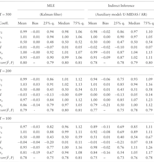
DGP2. For each combination of DGP parameters and sample size, we provide the results of the II procedure for parameter estimation and filtering of the latent factor path. As a bench-mark, we also provide the estimation and filtering results using the ML procedure based on the Kalman filter.10
InTable 1, we consider DGP1 where the single latent factor process is mildly persistent with autocorrelationq¼0.5. The finite sample performance of the II estimator is remark-ably good. First, it has only a small bias for most configurations. Second—as expected—the ML estimator based on the Kalman filter is more efficient, but the efficiency loss of the II estimator is rather limited. The bias of both the II and the MLE is more pronounced for parameterry, that is the volatility of the LF measurement error. For this parameter, the
effi-ciency loss of the II estimator compared to MLE is a bit larger. As expected, the dispersions of the estimators decrease with the sample sizeT.Moreover, the reprojection procedure provides rather accurate estimates of the latent factor values. Indeed, the average correla-tion between true and filtered factor values is about 0.80 for all sample sizes, which is close to the performance of the Kalman filter.
In unreported MC results, we compared the performance of the above II estimator— which uses the U-MIDAS/AR auxiliary model for HF/ LF data—with the performance of the II estimator using only the LF U-MIDAS specification as auxiliary model. The II estima-tor of the standard deviation parameter for the HF datarxbased on the LF U-MIDAS
aux-iliary model has a large bias. As shown inTable 1, this problem does not arise when we include HF data in the auxiliary model via the mixed frequency VAR specification. These findings confirm the intuition that using data at both frequencies provides a more informa-tive auxiliary model.
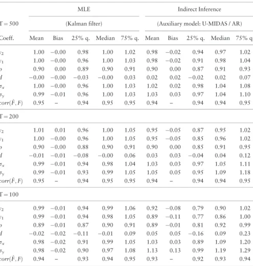
InTable 2, the autocorrelation of the latent factor in DGP1 is set equal toq¼0.9. Both the ML and II estimators have smaller dispersions in this MC design compared toTable 1. This effect is due to the more favorable signal-to-noise setting whenqis changed from 0.5 to 0.9 in our parameterization of the DGP. Indeed, with q¼0.9 the factor has a larger unconditional variance relative to the noise variance, which is fixed across the two cases. Hence, the signal-to-noise ratio is larger for the DGP inTable 2compared toTable 1.
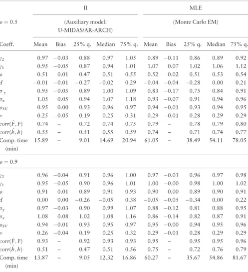
InTable 3we report the simulation results for DGP2, which features two latent factors, with loadings equal toc1¼ð1:0; 0:2Þ0 and c2¼ð0:2; 1:0Þ0:Compared to the one-factor
case inTables 1and2, the loadings are estimated rather precisely, with the dispersion of the loadings equal to 0.2 being larger than that of the loadings equal to 1.0. Also in this case we find that the II estimator has a very good performance, with the exception of the estimator of the LF volatilityry, which has a bias of around 20% for small sample sizes
(T¼200, 100), and a large dispersion. Nevertheless, the reprojection procedure produces accurate estimates of both factors. As expected, the factor which loads mainly on the HF observables (i.e. F2) is estimated more precisely (average correlation with the true factor
equal to 0.88 forT¼100) than the factor which loads mainly on the LF observables (aver-age correlation with the true factor equal to 0.74 forT¼100).
Table 1. MC simulations for the single-factor linear Gaussian state space model (persistence parameter of the latent factorq¼0:5)
MLE Indirect Inference
T¼500 (Kalman filter) (Auxiliary model: U-MIDAS / AR)
Coeff. Mean Bias 25% q. Median 75% q. Mean Bias 25% q. Median 75% q.
c2 0.99 0.01 0.94 0.98 1.06 0.98 0.02 0.86 0.97 1.10
c1 1.01 0.01 0.94 1.00 1.06 1.00 0.00 0.90 0.97 1.05
q 0.50 0.00 0.48 0.50 0.52 0.50 0.00 0.47 0.50 0.54
d 0.01 0.01 0.07 0.01 0.05 0.02 0.02 0.10 0.01 0.07
rx 1.00 0.00 0.92 1.01 1.07 0.99 0.01 0.87 1.04 1.15
ry 0.95 0.05 0.90 0.99 1.06 0.91 0.09 0.87 1.02 1.11
corrðF;^FÞ 0.80 – 0.79 0.80 0.81 0.78 – 0.78 0.79 0.80
T¼200
c2 0.99 0.01 0.86 1.01 1.12 0.94 0.06 0.75 0.93 1.09
c1 1.03 0.03 0.91 1.02 1.13 1.01 0.01 0.85 0.94 1.16
q 0.50 0.00 0.45 0.50 0.54 0.51 0.01 0.45 0.51 0.58
d 0.03 0.03 0.13 0.00 0.09 0.00 0.00 0.13 0.05 0.14
rx 0.97 0.03 0.84 1.00 1.12 1.00 0.00 0.85 1.07 1.23
ry 0.86 0.14 0.79 0.97 1.05 0.79 0.21 0.50 1.00 1.12
corrðF;^FÞ 0.79 - 0.78 0.80 0.81 0.77 – 0.75 0.78 0.79
T¼100
c2 0.97 0.03 0.82 0.96 1.12 0.89 0.11 0.69 0.85 1.11
c1 1.01 0.01 0.88 0.99 1.11 0.92 0.08 0.69 0.89 1.11
q 0.50 0.00 0.43 0.50 0.59 0.51 0.01 0.40 0.54 0.67
d 0.04 0.04 0.20 0.01 0.11 0.01 0.01 0.21 0.07 0.18
rx 0.95 0.05 0.77 1.00 1.16 0.98 0.02 0.76 1.11 1.26
ry 0.81 0.19 0.67 0.94 1.08 0.84 0.16 0.54 1.05 1.17
corrðF;^FÞ 0.78 – 0.75 0.78 0.81 0.75 – 0.73 0.76 0.78
Table 2. MC simulations for the single-factor linear Gaussian state space model (persistence parameter of the latent factorq¼0:9)
MLE Indirect Inference
T¼500 (Kalman filter) (Auxiliary model: U-MIDAS / AR)
Coeff. Mean Bias 25% q. Median 75% q. Mean Bias 25% q. Median 75% q.
c2 1.00 0.00 0.98 1.00 1.02 0.98 0.02 0.94 0.97 1.02
c1 1.00 0.00 0.96 1.00 1.03 0.98 0.02 0.91 0.98 1.04
q 0.90 0.00 0.89 0.90 0.91 0.90 0.00 0.87 0.91 0.93
d 0.00 0.00 0.03 0.00 0.03 0.02 0.02 0.02 0.02 0.07
rx 1.00 0.00 0.96 1.00 1.03 1.02 0.02 0.98 1.04 1.08
ry 0.99 0.01 0.96 1.00 1.03 1.03 0.03 0.97 1.04 1.10
corrðF;^FÞ 0.95 – 0.94 0.95 0.95 0.94 – 0.94 0.94 0.95
T¼200
c2 1.01 0.01 0.96 1.00 1.05 0.95 0.05 0.87 0.95 1.02
c1 1.00 0.00 0.96 1.00 1.05 0.95 0.05 0.85 0.96 1.02
q 0.90 0.00 0.88 0.90 0.91 0.90 0.00 0.85 0.91 0.95
d 0.01 0.01 0.08 0.00 0.06 0.03 0.03 0.04 0.04 0.12
rx 0.99 0.01 0.94 0.98 1.04 1.03 0.03 0.97 1.05 1.11
ry 0.99 0.01 0.93 0.99 1.05 1.05 0.05 0.95 1.09 1.18
corrðF;^FÞ 0.95 – 0.94 0.95 0.95 0.94 – 0.94 0.94 0.95
T¼100
c2 0.99 0.01 0.94 0.99 1.06 0.92 0.08 0.79 0.90 1.02
c1 0.99 0.01 0.94 0.98 1.05 0.89 0.11 0.77 0.86 1.00
q 0.89 0.01 0.87 0.90 0.91 0.89 0.01 0.81 0.92 0.99
d 0.02 0.02 0.11 0.01 0.09 0.05 0.05 0.16 0.09 0.23
rx 0.98 0.02 0.91 0.99 1.05 1.03 0.03 0.89 1.09 1.20
ry 0.98 0.02 0.90 0.97 1.08 1.13 0.13 0.99 1.19 1.29
corrðF;^FÞ 0.94 – 0.93 0.94 0.95 0.93 – 0.92 0.93 0.94
T able 3. MC simulations for the two-factor linear Gaussian state space model II T ¼ 500 T ¼ 200 T ¼ 100 Coeff. Mean Bias 25% q. Median 75% q. Mean Bias 25% q. Median 75% q. Mean Bias 25% q. Median 75% q.
c2;1
0.17 0.03 0.00 0.00 0.37 0.16 0.04 0.00 0.00 0.33 0.18 0.02 0.00 0.12 0.36
c2;2
0.98 –0.02 0.92 0.99 1.05 0.98 0.02 0.87 0.98 1.10 1.00 0.00 0.85 1.00 1.17
c1;1
0.99 0.01 0.91 0.98 1.05 1.05 0.05 0.94 1.03 1.17 1.01 0.01 0.81 0.99 1.22
c1;2
0.21 0.01 0.00 0.30 0.37 0.22 0.02 0.00 0.26 0.38 0.15 0.05 0.00 0.12 0.27 q 0.90 0.00 0.87 0.90 0.92 0.88 0.02 0.84 0.89 0.92 0.88 0.02 0.85 0.89 0.93 d 0.01 0.01 0.07 0.00 0.07 0.01 0.01 0.10 0.01 0.10 0.05 0.05 0.18 0.02 0.10 rx 1.00 0.00 0.93 1.01 1.05 1.00 0.00 0.92 1.01 1.09 0.94 0.06 0.85 1.00 1.09 ry 0.93 0.07 0.85 0.98 1.09 0.76 0.24 0.52 0.83 1.07 0.81 0.19 0.36 0.96 1.21 corr ð
^F1
; F1 Þ 0.78 – 0.76 0.78 0.80 0.76 – 0.74 0.76 0.79 0.74 – 0.72 0.76 0.78 corr ð
^F2
; F2 Þ 0.92 – 0.91 0.92 0.92 0.91 – 0.90 0.92 0.93 0.88 – 0.89 0.92 0.93 This table reports mean, bias, and 25%, 50%, 75% quantiles of the distribution of the II estimator in 1000 MC replications. The data generating process is DGP2 in Section 4.1, cor-responding to a mixed frequency linear state space model with two independent AR(1) latent factors, m ¼ 3, and stock sampling of the LF variable. The true values of the parameters are c1 ¼ð 1 : 0 ; 0 : 2 Þ 0; c2 ¼ð 0 : 2 ; 1 : 0 Þ 0; q ¼ 0 : 9, d ¼ 0, ry ¼ rx ¼ 1. The simulated samples have size T ¼ 500 (left), T ¼ 200 (middle), T ¼ 100 (right). The auxiliary model for the II esti-mator is a U-MIDAS regression for LF data with
~Kx
¼
~Ky
Overall, the results inTables 1–3are remarkably impressive, since they show that the performance of the II procedure is rather close to the efficient benchmark in the linear Gaussian state space model.
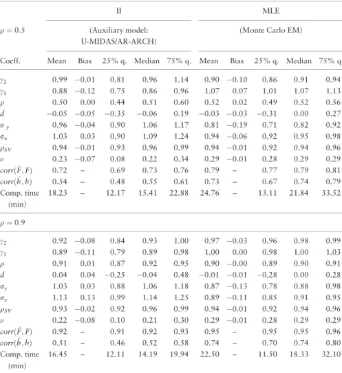
4.3 Monte Carlo Results for the State Space SV Model
We now consider the more challenging state space model with SV in DGP3.Tables 4and5 report the results of Monte Carlo simulations comparing the II estimator with the MLE (implemented via a simulation-based EM algorithm) for sample sizesT¼500 andT¼200 respectively. These tables compare the two estimation methods on the basis of (i) statistical criteria—mean/bias/quantiles of sampling distributions, (ii) filtering accuracy—both for conditional mean and for volatility factors, and (iii) computational time. Compared to the linear Gaussian state space model in DGP1, the structural model now has two additional parameters, which are the autoregressive coefficientqSVand the volatility parameter of
the log SV process. A first encouraging finding is that the estimation results for parameters c1,c2,q,d,ry,rxare comparable to those of the Gaussian state space model displayed in
Tables 1and2, with slightly larger dispersions inTables 4and5, as expected. The latter effect is more pronounced for parameterd, the autoregressive coefficient of the LF measure-ment error, for both the II estimator and the MLE. The SV parametersqSVandare
esti-mated with rather small biases. Note that sample size T¼200 corresponds to 600 HF observations, and for such sample sizes the estimation of ARCH and SV specifications can be inaccurate, even in the absence of latent factors in the mean. Yet, comparing the distri-butions of II and ML estimates, we observe that also in the SV case the efficiency loss of the former estimator is limited.
It is worth noting that the reprojection method provides rather accurate estimates of the latent factor values also in the SV model. Results are less good for the log volatility factor (average correlation between estimated and true factor values equal to 0.55 for sample size
T¼500 in the design with q¼0:5). This result is not surprising, because there is no obvious choice for the transformations of the observable variables, whose linear combina-tion provides the best approximacombina-tion of the condicombina-tional expectacombina-tion of the volatility factor in this nonlinear state space model. InTables 4and5we use current and past values of log squared HF residuals, but other choices could yield better results.
The II procedure provides a substantial reduction in computational time compared to the simulation-based EM procedure used to obtain the ML estimates. For instance, the computation of the II estimates for one Monte Carlo repetition in the SV design with q¼0:5 and sample size T¼200 takes on average about 18 minutes, against the 24 minutes required on average for the ML estimates. The difference is larger with sample size T¼500, for which the average computational times are 16 minutes for II and 61 minutes for ML. Here, the computational time for the II procedure is less than 21 minutes in 75% of the MC replications, while the computational time for ML is more than one hour in more than 25% of the MC replications. Sample sizes such asT¼500 or even larger are often encountered in financial datasets, if the lower frequency is weekly or monthly.
Table 4. MC simulations for the SV model (sample sizeT¼500)
II MLE
q¼0:5 (Auxiliary model:
U-MIDAS/AR-ARCH)
(Monte Carlo EM)
Coeff. Mean Bias 25% q. Median 75% q. Mean Bias 25% q. Median 75% q.
c2 0.97 0.03 0.88 0.97 1.05 0.89 0.11 0.86 0.89 0.92
c1 0.95 0.05 0.87 0.94 1.01 1.07 0.07 1.02 1.06 1.12
q 0.51 0.01 0.47 0.51 0.55 0.52 0.02 0.51 0.53 0.54
d 0.01 0.01 0.27 0.02 0.29 0.04 0.04 0.28 0.00 0.21
ry 0.95 0.05 0.89 1.00 1.09 0.83 0.17 0.75 0.84 0.91
rx 1.05 0.05 0.94 1.07 1.18 0.93 0.07 0.91 0.94 0.96
qSV 0.95 0.00 0.93 0.96 0.97 0.94 0.01 0.93 0.94 0.95
0.25 0.05 0.19 0.25 0.31 0.29 0.01 0.28 0.29 0.29
corrðF;^FÞ 0.74 – 0.72 0.74 0.75 0.79 – 0.78 0.79 0.80
corrðh;^hÞ 0.55 – 0.51 0.55 0.59 0.74 – 0.71 0.74 0.77 Comp. time
(min)
15.89 – 9.01 14.69 20.94 61.05 – 38.49 54.11 78.05
q¼0:9
c2 0.96 0.04 0.91 0.96 1.00 0.97 0.03 0.96 0.97 0.98
c1 0.95 0.05 0.90 0.96 1.01 1.00 0.00 0.98 1.00 1.02
q 0.91 0.01 0.89 0.91 0.93 0.90 0.00 0.89 0.90 0.91
d 0.00 0.00 0.26 0.05 0.38 0.05 0.05 0.34 0.00 0.22
ry 0.97 0.03 0.90 0.99 1.07 0.88 0.12 0.81 0.88 0.95
rx 1.08 0.08 1.02 1.08 1.16 0.86 0.14 0.82 0.87 0.91
qSV 0.94 0.01 0.93 0.95 0.97 0.95 0.00 0.94 0.95 0.96
0.26 0.04 0.19 0.25 0.32 0.29 0.01 0.28 0.29 0.29
corrðF;^FÞ 0.93 – 0.92 0.93 0.93 0.95 – 0.95 0.95 0.96
corrðh;^hÞ 0.51 – 0.47 0.51 0.56 0.75 – 0.72 0.76 0.79 Comp. time
(min)
13.87 – 9.05 12.32 16.86 60.27 – 35.67 54.86 81.67
This table reports mean, bias, and 25%, 50%, 75% quantiles of the distribution of the II (left) and ML (right) estimators in 200 MC replications. The data generating process is DGP3 in Section 4.1, corresponding to a mixed frequency SV model with a single AR(1) latent factor in the mean, an AR(1) log SV process,m¼3, and stock sampling of the LF variable. The true values of the parameters are c1¼c2¼1, d¼0, ry¼rx¼1;qSV¼0:95; ¼0:3. The autoregressive coefficient of the factor in the mean isq¼0:5 in the upper panel andq¼0:9 in the lower panel. The simulated samples have sizeT¼500. The auxiliary model for the II estimator is a U-MIDAS regression for LF data withK~x¼K~y¼4 and an ARð9Þ ARCHð10Þmodel for the HF data (seeEquation (2.10)), with the correlation between the errors of the two equations as a free auxili-ary parameter. The II estimator uses a single long simulated sample of the structural model (S¼1 and TS
Table 5. MC simulations for the SV model (sample sizeT¼200)
II MLE
q¼0:5 (Auxiliary model:
U-MIDAS/AR-ARCH)
(Monte Carlo EM)
Coeff. Mean Bias 25% q. Median 75% q. Mean Bias 25% q. Median 75% q.
c2 0.99 0.01 0.81 0.96 1.14 0.90 0.10 0.86 0.91 0.94
c1 0.88 0.12 0.75 0.86 0.96 1.07 0.07 1.01 1.07 1.13
q 0.50 0.00 0.44 0.51 0.60 0.52 0.02 0.49 0.52 0.56
d 0.05 0.05 0.35 0.06 0.19 0.03 0.03 0.31 0.00 0.27
ry 0.96 0.04 0.90 1.06 1.17 0.81 0.19 0.71 0.82 0.92
rx 1.03 0.03 0.90 1.09 1.24 0.94 0.06 0.92 0.95 0.98
qSV 0.94 0.01 0.93 0.96 0.99 0.94 0.01 0.92 0.94 0.96
0.23 0.07 0.08 0.22 0.34 0.29 0.01 0.28 0.29 0.29
corrðF;^FÞ 0.72 – 0.69 0.73 0.76 0.79 – 0.77 0.79 0.81
corrðh;^hÞ 0.54 – 0.48 0.55 0.61 0.73 – 0.67 0.74 0.79 Comp. time
(min)
18.23 – 12.17 15.41 22.88 24.76 – 13.11 21.84 33.52
q¼0:9
c2 0.92 0.08 0.84 0.93 1.00 0.97 0.03 0.96 0.98 0.99
c1 0.89 0.11 0.79 0.89 0.98 1.00 0.00 0.98 1.00 1.03
q 0.91 0.01 0.87 0.92 0.95 0.90 0.00 0.89 0.90 0.91
d 0.04 0.04 0.25 0.04 0.48 0.01 0.01 0.28 0.00 0.28
ry 1.03 0.03 0.88 1.06 1.18 0.87 0.13 0.78 0.88 0.98
rx 1.13 0.13 0.99 1.14 1.25 0.89 0.11 0.85 0.91 0.95
qSV 0.93 0.02 0.92 0.96 0.99 0.94 0.01 0.92 0.94 0.96
0.22 0.08 0.10 0.21 0.30 0.29 0.01 0.28 0.29 0.29
corrðF;^FÞ 0.92 – 0.91 0.92 0.93 0.95 – 0.95 0.95 0.96
corrðh;^hÞ 0.51 – 0.46 0.52 0.58 0.74 – 0.70 0.74 0.80 Comp. time
(min)
16.45 – 12.11 14.19 19.94 22.50 – 11.50 18.33 32.10
This table reports mean, bias, and 25%, 50%, 75% quantiles of the distribution of the II (left) and ML (right) estimators in 200 MC replications. The data generating process is DGP3 in Section 4.1, corresponding to a mixed frequency SV model with a single AR(1) latent factor in the mean, an AR(1) log SV process,m¼3, and stock sampling of the LF variable. The true values of the parameters are c1¼c2¼1, d¼0, ry¼rx¼1;qSV¼0:95; ¼0:3. The autoregressive coefficient of the factor in the mean isq¼0:5 in the upper panel andq¼0:9 in the lower panel. The simulated samples have sizeT¼200. The auxiliary model for the II estimator is a U-MIDAS regression for LF data withK~x¼K~y¼4 and an ARð9Þ ARCHð10Þmodel for the HF data (seeEquation (2.10)), with the correlation between the errors of the two equations as a free auxili-ary parameter. The II estimator uses a single long simulated sample of the structural model (S¼1 and TS
5 Empirical Study
We present an empirical application of our model to the problem of forecasting at short horizons the Euro-area quarterly GDP growth using monthly macroeconomic indicators.
5.1 Data and Model Specification
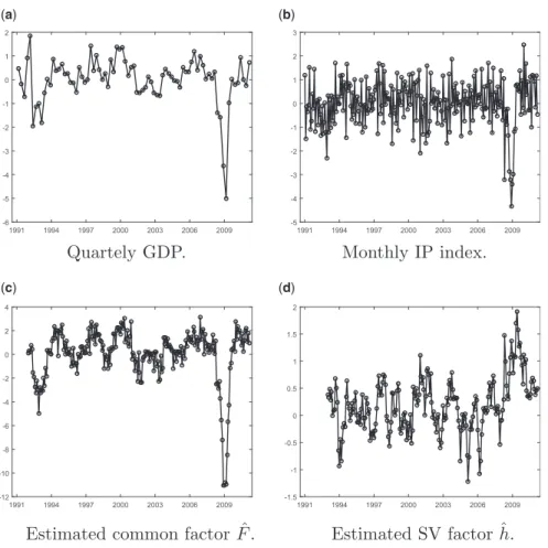
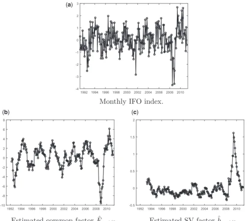
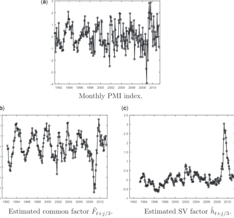
The dataset is the same as the one considered in the empirical study of Marcellino, Porqueddu, and Venditti (2016).11The data consist of the quarterly GDP growth rates for the Euro-area (GDP) observed from 1991-Q1 to 2011-Q1, and the monthly observa-tions for the same period, that is from 1991-M1 to 2011-M3, for the following eight macroeconomic indicators: (1) the aggregate European Industrial Production index for all sectors of the European economy: IP; (2) the European Industrial Production index for “Pulp and Paper sector”: IP-Pulp/Paper; (3) the Germany IFO Business Climate index: IFO; (4) the Euro-area Economic Sentiment index: ESI; (5) the Euro-area Composite Purchasing Manager index: PMI; (6) the bilateral dollar-euro exchange rate, measured as year-on-year percentage growth: EXC; (7) the difference between three-month and 10-year U.S. Treasury bond yield: SPR; and (8) the University of Michigan consumer sentiment index for the United States: MICH. In line with the empirical study ofBai, Ghysels, and Wright (2013), we consider the first difference of the series (3) to (8) to induce stationarity, and we normalize all series by their full sample mean and standard deviation.12
We estimate the mixed-frequency SV model defined as DGP 3 in Section 4 and the linear Gaussian factor model defined as DGP 1 on eight different pairs of mixed fre-quency observables.13In each model we include GDP as the LF observable, and one of the eight monthly indicators listed above as the HF variable. We assume the presence of one HF latent factor (nf¼1), and that the observed quarterly GDP is the sum of three
unobservable monthly growth rates:yt¼ytþyt1=3þyt2=3. Thus, we havem¼3 and
the LF variable is flow sampled. We estimate the SV model by the II procedure, using the same auxiliary model as in the MC simulations of Section 4, and deploy the II estimates in the reprojection procedure to filter the latent factors. We estimate the Gaussian state space model without SV by adapting the Kalman filter for periodic state space models proposed in Bai, Ghysels, and Wright (2013) to accommodate flow sampling (see Appendix C).
5.2 Estimation and In-Sample Explanatory Power
Before performing the forecasting exercise, we discuss the estimation results of the models for the entire data sample ending in 2011-Q1. InTable 6, we report the values of theR2of
the regression of both GDP and the five monthly indicators (1)–(5) on the filtered values of
11 We thank M. Marcellino, M. Poqueddu, and F. Venditti for sharing their dataset with us.
12 Augmented Dickey–Fuller tests failed to reject the null hypothesis of a unit root for series (3) to (8).