Obesity and Health-Related Decisions: an Empirical Model of Weight Status for Young Adults in the US
Leonardo Fabio Morales Zurita
A dissertation submitted to the faculty of the University of North Carolina at Chapel Hill in partial fulfillment of the requirements for the degree of Doctor of Philosophy in the Department of Economics.
Chapel Hill 2013
Approved by:
David Guilkey
Donna Gilleskie
Klara Peter
Helen Tauchen
c 2013
Abstract
LEONARDO FABIO MORALES ZURITA: Obesity and Health-Related Decisions: an Empirical Model of Weight Status for Young Adults in the US.
(Under the direction of David Guilkey.)
Obesity is widely accepted as one of the main causes of premature death, and the causal
relationship between obesity and several of the most deadly chronic diseases is a consensus
in the medical and public health literature. Obesity in the United States has recently been
recognized as a public health concern and a social problem because the rise in the obesity
prevalence rate has been stunning over the past three decades. Using AddHealth, a longitudinal
study of teenagers and young adults in the United States, I estimate a comprehensive dynamic
model of obesity determination that assumes as endogenous several factors mentioned in the
literature as obesity determinants: physical activity, smoking, a proxy for food consumption,
and childbearing. Two additional endogenous decisions included in the model are
career-related decisions and residential location decisions. The first is included because it determines
the intensity, in terms of energy expenditure, of individuals’ daily main activities. The second
is included because it determines the built environments in which individuals live. I specify
reduced form equations for all these endogenous demand decisions, together with an obesity
structural equation. The whole system of equations is jointly estimated by full information
maximum likelihood methods. The errors in all equations are assumed to be correlated with
each other in the estimation. I use the discrete factor random effects estimation method to
model this unobserved heterogeneity. Using the empirical model to study the mechanisms
behind the determination of obesity, I am able to quantify the effect on the probability of
obesity of several individual decisions after controlling for the endogenous nature of those
decisions. This research provides evidence of important effects of physical activity on the
reduction in the probability of obesity for young men and women. In addition, I found evidence
of a small but significant negative effect of the availability of a set of neighborhood amenities on
to the literature, because these results are obtained within a framework in which the residential
Acknowledgments
I would like to express my deep gratitude to my adviser, David Guilkey, for his guidance and
support in every single step of the process of developing this dissertation. His feedback and
advice made this research possible. I would like to thank my committee members Donna
Gilleskie, Penny Gordon-Larsen, Helen Tauchen, and Klara Peter for the immense help they
provided in this research. I am grateful for having the influence of these five people in my life
because all of them are examples for me to follow as researchers and professors.
I dedicate this dissertation to the eight women of my life. My wife, my grandma, my four
aunts, my mother and my mother in law. All of them have contributed in many different
ways to whatever I have accomplished in life, including finishing this dissertation. In regard
to the dissertation, I should say that my lovely wife deserves a special recognition. She was
my partner along the way, and just for tolerating my mood in the difficult times of the PhD
Table of Contents
List of Tables . . . ix
List of Figures . . . x
1 Introduction . . . 1
2 Background Literature . . . 5
3 Data . . . 9
3.1 The AddHealth Study . . . 9
3.2 Contextual Information and Neighborhood Characteristics . . . 10
4 Theoretical Motivation . . . 12
4.1 Simple Static Model . . . 12
4.2 Dynamic Framework . . . 18
5 Empirical Model . . . 25
5.1 Error Structure . . . 26
5.2 Empirical Equations . . . 27
5.2.1 Residential Location Decisions . . . 27
5.2.2 Career Related Decisions . . . 32
5.2.3 Simultaneous Choices and Final Health Outcome . . . 36
5.3 Initial Conditions and Identification Issues . . . 40
5.3.1 Sources of Identification . . . 40
5.3.2 Initial Conditions . . . 41
5.4.1 Likelihood Function . . . 43
5.4.2 Missing Values and Attrition . . . 44
6 Results . . . 46
6.1 Summary Statistics and Sample Description . . . 46
6.2 Estimations Results of the Model for Women . . . 48
6.2.1 Obesity Equation . . . 48
6.2.2 Input Equations Estimation Results for Women . . . 51
6.3 Simulations and Fit of the Model for Women . . . 60
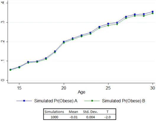
6.3.1 Fit of the Model . . . 61
6.3.2 Simulated Changes of the Obesity Prevalence Rate . . . 62
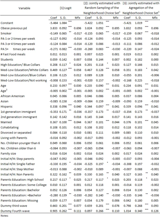
6.4 Estimations Results of the Model for Men . . . 66
6.4.1 Obesity Equation . . . 66
6.4.2 Input Equations Estimation Results for Men . . . 68
6.5 Simulations and Fit of the Model for Men . . . 77
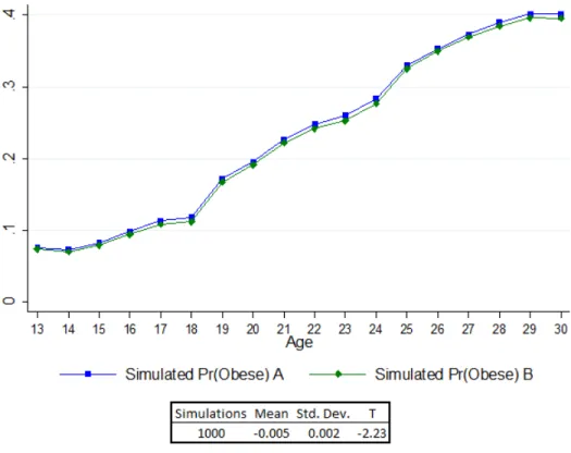
6.5.1 Fit of the Model for Males . . . 77
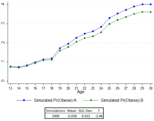
6.5.2 Simulated Changes of the Obesity Prevalence Rate . . . 78
6.6 Remarks on the Validity of Exclusion Restrictions . . . 81
7 Conclusion and Final Remarks . . . 83
7.1 Conclusion . . . 83
Appendices . . . 88
Appendix A. Unobserved Heterogeneity Parameters . . . 88
Appendix B1. Residential Location Model for Women . . . 89
Appendix B2. Residential Location Model for Men . . . 90
Appendix B3. Residential Location Model Conditional Component . . . 91
Appendix C1. Career Related Decision Model for Women . . . 92
Appendix C2. Career Related Decision Model for Men . . . 94
Appendix D. Neighborhood Characteristics Summary Statistics . . . 96
Appendix F. Neighborhood Type Clusters . . . 98
Appendix G. Initial Conditions Estimation Results for Women . . . 99
Appendix H. Initial Conditions Estimation Results for Men . . . 101
List of Tables
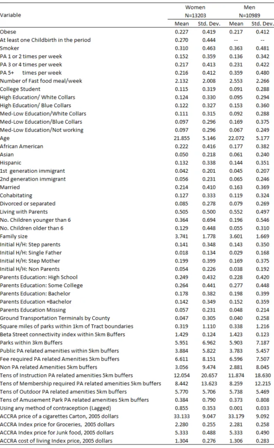
1 Summary Statistics . . . 47
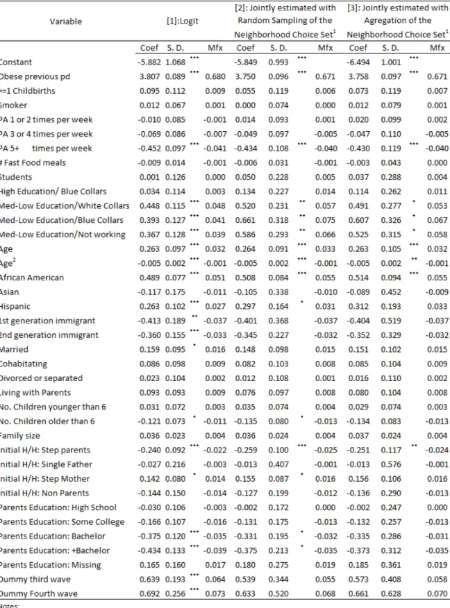
2 Weight Status Estimation Results for Women . . . 49
3 Physical Activity Estimation Results for Women . . . 54
4 Smoking, Pregnancies, and Fast Food Meals Estimation Results . . . 57
5 Weight Status Estimation Results for Men . . . 67
6 Physical Activity Estimation Results for Men . . . 71
7 Smoking and Fast Food Meals Estimation Results . . . 75
A1 Unobserved Heterogeneity Parameters for Women’s Equations . . . 88
A2 Unobserved Heterogeneity Parameters for Men’s Equations . . . 88
B1 Residential Location Model for Women . . . 89
B2 Residential Location Model for Men . . . 90
B3 Residential Model Conditional Component . . . 91
C1 Career Related Decision Model for Women . . . 92
C2 Career Related Decision Model for Men . . . 94
D Neighborhood Characteristics . . . 96
E Cluster for CRD Summary Statistics . . . 97
F Clusters Summary Statistics . . . 98
G Initial Conditions Estimation Results for Women . . . 99
H Initial Conditions Estimation Results for Men . . . 101
D1 Data Appendix 1 . . . 102
D2 Data Appendix 2 . . . 103
List of Figures
1 Model Predictions of Female Obesity Prevalence . . . 62
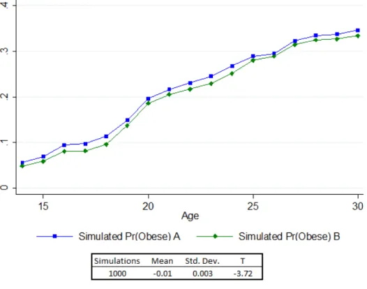
2 Simulated Effects of Intense Physical Activity in High School . . . 63
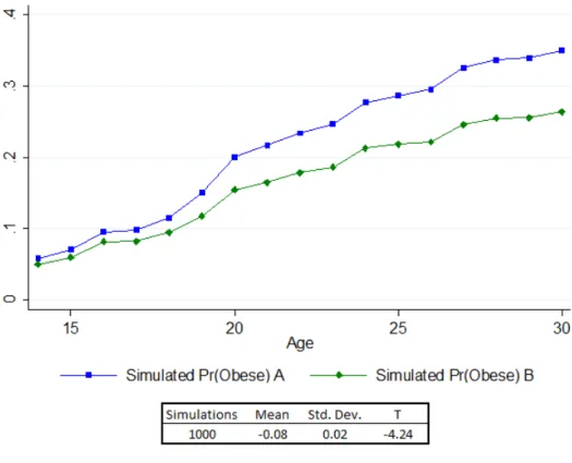
3 Simulated Effects of Constant Intense Physical Activity . . . 64
4 Simulated Effects of One Standard Deviation Increase in Amenities . . . 66
5 Model Predictions of Male Obesity Prevalence . . . 77
6 Simulated Effects of Intense Physical Activity in High School . . . 79
7 Simulated Effects of Constant Intense Physical Activity . . . 80
Chapter 1
Introduction
In recent years economists, especially in the field of health economics, have shown an increased
interest in health outcomes associated with the weight status of individuals. This growth of
interest is not surprising because obesity has been strongly related in the medical and public
health literature to chronic diseases such as diabetes type II, heart disease, and hypertension
(Mokdad et al., 2001; Must et al., 1999). In addition, the prevalence of obesity has risen to
such a degree in developed countries that it is now considered an epidemic. For the United
States, in 2008 the prevalence rate of obesity was 32.2% among adult men and 35.5% among
adult women (Flegal et al., 2010). These rates imply a dramatic increase in the last three
decades when compared with the prevalence of 12.7% for men and 17% for women measured
in the late 1970s (Eid et al., 2008).
There is an ongoing debate about the factors that cause obesity and that have contributed
to the remarkably high obesity prevalence in the U.S. Several studies in the literature on
obesity have focused on the effect that relative prices of calories and physical activity have
on the determination of weight status. More in line with the purposes of this research are
the efforts that have been made to find causal links between individual choices and obesity
measures. The obesity causal factors usually taken into account in the literature are smoking,
physical activity, diet, and similar individual lifestyle descriptors. Some of these papers have
noted that individual choices usually associated with obesity are endogenous (Rashad, 2006;
Ng et al., 2010). Another factor that has been explored in research about the determinants of
obesity is the environment in which individuals perform their daily activities. Recent literature
in increasing energy consumption and decreasing energy expenditure (Papas, 2007). In other
words, neighborhoods may affect the demand for exercise and diet, and thereby have an impact
on obesity.
In this dissertation I propose a theoretical and empirical framework for modeling weight
status and additional endogenous individual behaviors that may play important roles in the
determination of an individual’s weight. Within this framework, the probability of being
obese is the result of endogenous choices, exogenous factors, and an unobserved heterogeneity
component. Econometrically, the estimation strategy used here consists of the specification of
a system of equations that include weight status and the set of endogenous choices. The entire
system is jointly estimated by full information maximum likelihood methods. The estimation
technique also incorporates unobserved heterogeneity that is correlated across the equations
by using a semi-parametric method that does not require assumptions about its distribution.
In addition to taking into account lifestyle choices (smoking, physical activity, etc.) that
have been linked to obesity in the literature, this research also incorporates two major
deci-sions in individuals’ lives: career-related decideci-sions and residential-location decideci-sions. Inclusion
of these choices is an important extension of obesity models for two reasons. One is that
individual energy expenditure levels depend greatly upon the kind of career path a person
decides to follow, because there are different levels of physical activity for different jobs,
differ-ent resources for healthier lifestyles in differdiffer-ent professions, etc. The second is that residence
location decisions determine the characteristics and resources of neighborhoods in which
indi-viduals live. These characteristics and resources may encourage indiindi-viduals to increase their
energy expenditure levels by engaging in physical activity. By modeling the residential location
decision, I am able to control for the potential endogeneity of neighborhood characteristics in
the decision to perform any sort of physical activity. This is one of the most important
con-tributions of this research to the literature. Modelling residential decisions is crucial because
the effect of neighborhood characteristics on obesity will be biased if researchers ignore the
fact that individuals self-select themselves into their neighborhoods. This research is a step
forward in this direction because, up to this author’s knowledge, there have been no attempts
Using the estimated model, I measure the contribution of several endogenous factors to
the probability of an individual being obese. Another special feature of this model is that it
allows me to test the hypothesis that different neighborhood amenities have different impacts
on individuals’ endogenous lifestyle decisions, such as the performance of physical activity.
Therefore, this research may contribute to the recent debate about the influence of built
environments on the propensity to become obese. Several findings of a causal relationship
with regard to this hypothesis have been criticized for assuming that environmental factors are
exogenous. Critics are motivated by the facts that 1) the environment is usually represented by
neighborhood characteristics and 2) these characteristics are endogenous, because residential
selection is an individual’s choice.
Although the existence of an obesity epidemic in the United States is well established, the
kind of public policy that would be effective in dealing with the problem remains unclear.
The present research contributes to this debate by proposing a comprehensive model of
obe-sity determination. This model allows exploration of the contribution of several endogenous
decisions on the probability of being obese in a framework that controls for the endogeneity
of these choices. With the estimated model I perform some experiments that allow us to see
what the evolution of the obesity prevalence rate would have been if individuals had decided to
have healthier lifestyles. In addition, I test a set of neighborhood amenities to see if they have
any significant impact upon encouraging healthy behaviors, and the effect of this influence on
obesity prevalence.
I find evidence of a significant reduction in the obesity prevalence rate for adult females and
males derived from a hypothetical situation in which they perform intense physical activity
when they are high school students. I also found evidence that a generalized, continuous
practice of intense physical activity would produce big falls in the adult obesity prevalence
rate. In addition, using the model estimation results, I test if a set of neighborhood amenities
has any significant impact upon the encouragement of physical activity. After controlling for
the endogeneity of neighborhood amenities, I find that most neighborhood amenities are not
significant in terms of encouraging residents’ physical activity. Nevertheless, an increase in
Chapter 2
Background Literature
There is an increasing amount of literature about obesity in several disciplines of the social
sciences; the recent interest in this topic has two main explanations. First, it is one of the most
important public policy concerns in the US nowadays; according with the Center for Disease
Control, it is the second leading cause for premature death, after smoking (Mokdad, Marks,
Stroup, and Gerberding, 2000). The amount of resources spent every year in medical care to
obesity and its consequences is high and has been increasing with the obesity prevalence rate
(Wolf and Colditz, 1998; USDHHS, 2001; Bhattacharya and Sood, 2006; Folmann et al, 2006).
The second reason is that the growth of obesity in the US during the last three decades was
surprisingly high. Between 1960 and 1980 obesity prevalence rates in US were relatively stable
(Rashad and Grossman, 2004), but after 1980 the prevalence rates more than doubled their
original levels. Explaining this accelerated growth of obesity prevalence is a real puzzle and
a very interesting question for many social scientists. In order to solve this puzzle, standard
tools from economics could be very useful. This issue has opened a recent research interest
that could be grouped under the terminology of ”economics of obesity”.
From an economic perspective, many elements could have contributed to the sharp growth
in obesity. Recent literature has focused on the role that changes in relative price and cost
of food may play. One of the first papers to formally state a hypothesis and prove some
of its implications was Cutler et al. (2003), in which aggregate data was used to conclude
that the recent obesity epidemic is explained by a reduction in the time cost of household
meal production (as a result of this reduction, there has been an increase in the quantity
societies is another factor associated in the literature with the high obesity prevalence observed
in recent decades (Lakdawalla & Philipson, 2002; Philipson & Posner, 1999). An example of
this branch of the literature is Lakdalla, Philipson, and Bhattacharya’s (2005) hypothesis that
technological change has simultaneously lowered the cost per calorie and raised the cost of
physical activity by making agricultural production more efficient and jobs more sedentary
(Lakdalla et al., 2005). The contribution of technological change to obesity was also portrayed
in Lakdawalla and Philipson (2002), a paper that presented evidence of the existence of an
inverse relationship between Body Mass Index (BMI) and job strenuousness.
A recent series of papers has extended this research line by exploring the determinants
of obesity and BMI as health outcomes derived from individual characteristics and choices.
Usually these choices are variables that describe aspects of an individual’s lifestyle (French et
al., 2010, Grossman & Saffer 2004; Rashad 2006; Ng et al., 2012). In general terms, all of these
papers specified obesity or BMI equations using micro-data. Therefore, in this sub-branch of
the literature one could make the distinction between papers that control or do not control
for potential endogeneity bias. Grossman and Saffer (2004), for example, did not address any
possible endogeneity issue in regard to the elements they used as explanatory variables. Rather
than specific individuals’ decisions, the variables they included in their BMI equations were
prices and contextual variables that could be exogenous to some extent.
Other papers, such as Rashad (2006), French et al.(2010) and Ng et al. (2012) have
specified the weight status equation in terms of individual decisions; in doing so, they assumed
those decisions are endogenous and therefore implemented an empirical strategy to correct for
the endogeneity bias. In the case of Rashad 2006, the author controlled for the endogeneity
of smoking, calorie intake, and physical activity by using instrumental variables estimation
methods. French et al. (2010) took advantage of the longitudinal nature of their data and
used fixed effect panel methods to get rid of time-invariant unobserved heterogeneity that
could be correlated with the variables of interest. Ng et al. (2012) estimated a dynamic
model of weight using longitudinal data from China. To control for the endogeneity of the
individual choices included in the model (i.e., smoking, drinking, physical activity, and diet),
factors such as urbanicity and prices.
Another branch of the literature has sought to identify the links between high levels of
obesity prevalence and characteristics of the environments in which individuals live. The main
hypothesis of the papers in this branch is that built environments may encourage individuals’
physical activity and thereby have an impact on obesity. One variable that has caught the
attention of many researchers is ”urban sprawl,” usually defined as the expansion of cities and
their suburbs to rural areas. Researchers from numerous disciplines have tested the
hypoth-esis of a significant relationship among urban sprawl, physical activity, and obesity (Ewing,
Schmid, Killingsworth, Zlot, & Raudenbush, 2003; Giles-Corti, Macintyre, Clarkson, Pikora,
& Donovan, 2003; Glaeser & Kahn, 2004; Lathey, Guhathakurta, & Aggarwal, 2009; Saelens,
Sallis, Black, & Chen 2003). Other researchers have used wider measures of built environment
beyond urban sprawl.
The built environment can be understood as a major component of community design; as
such it is comprised of aspects such as buildings, transportation systems, parks, and greenways
(Boone-Heinonen et al., 2009). Several papers have sought to measure the relationship between
weight or energy expenditure measures and neighborhood density of physical-activity-related
facilities (Boone-Heinonen & Gordon-Larsen, 2009; Gordon-Larsen, Nelson, Page, & Popkin,
2006). These works have stated a clear hypothesis, namely that neighborhood amenities and
characteristics can improve the health of the population by encouraging positive health habits
in the community.
Some of the papers mentioned in the previous paragraph noted the importance of
con-trolling for the endogeneity of neighborhood characteristics. Given the ability of households
to choose a neighborhood that matches their interest in health issues, this variable should be
treated as endogenous. In other words, the tendency of healthy people to look for healthy
neighborhoods to live in can be interpreted as a self-selection process. The usual strategy
of some researchers for controlling for the endogeneity of neighborhood characteristics is to
perform some kind of fixed effects estimation method (Boone-Heinonen et al., 2010; Eid et al.,
2008). A good example of papers based on fixed effects methodologies is Eid et al. (2008);
estimator. Their results rejected the hypothesis of a significant relationship between urban
sprawl and obesity. For a very comprehensive review of the evolution of this literature, the
reader may refer to Boone-Heinonen et al. (2009).
The present research shares the common conception of several of the papers mentioned
above, the idea that weight status can be modeled as a health production function that is
determined by individual characteristics and choices. Some papers in the literature on obesity
have focused on identifying the effect of lifestyle choices on weight status, whereas others have
focused on identifying the effects of neighborhood characteristics (which are determined by the
residential location decision) on weight status. In the present research, I propose a
comprehen-sive, dynamic model in which weight status appears as the combined result of lifestyle choices
and recognizes that neighborhood amenities help determine the levels of physical activity that
individuals decide to perform. Therefore, this dissertation can be seen as a bridge between
these two types of obesity research. I control for the endogeneity of these choices by estimating
the model jointly and by allowing errors to be correlated across equations. One of the choices
that the individual is allowed to make in this model is the residential location decision. By
explicitly modeling residential decisions I can control for the endogeneity of the neighborhood
characteristics that are directly derived from it. The methodology itself is another contribution
of the present research to the literature on obesity because in almost all cases, endogeneity
issues have been controlled using instrumental variables or fixed effects models. These
ap-proaches have some limitations, such as the inability to account for time-varying unobserved
Chapter 3
Data
The main source of information used in this study is The National Study of Adolescent Health
(AddHealth). One of the main characteristics of this study is its comprehensive contextual
information on the characteristics of the neighborhoods in which the respondents live.
Be-cause neighborhood characteristics are important in the present research, a subsection below
is devoted to explaining the contextual information available in AddHealth and the definition
of neighborhood used herein. A general explanation of the AddHealth study dataset is also
provided.
3.1 The AddHealth Study
The National Study of Adolescent Health (AddHealth) is a longitudinal survey that began
with a nationally representative sample of high school students in grades 7 to 12 during the
1994 and 1995 school years. Respondents were followed after the first wave of data collection
and were interviewed three additional times. AddHealth explores adolescents’ health-related
behaviors and keeps track of them into young adulthood. Something unique about AddHealth,
and very crucial for the present study, is that it contains very good information on the activities
that respondents perform during their ”active” leisure time. This information is important
because the relationship between weight status and physical activity is where policy variables
of interest may demonstrate influence. Other special features of AddHealth include its great
diversity in terms of ethnic backgrounds (4,400 African Americans, 3,400 Hispanics, 1,500
Asians). In addition, it includes special oversamples of important populations such as sibling
and Chinese. These special oversamples were also very important for the present study because
they made it easier to identify and measure the existence of racial and ethnic health disparities..
The first wave (Wave I) of AddHealth, collected in 1995, consisted of 20,745 high school
students in grades 7 through 12. The second wave (Wave II), collected in 1996, included 14,738
of the original Wave I respondents. The third wave (Wave III), collected in 2001, included
15,197 original Wave I respondents, most between 18 and 26 years of age. The last wave (Wave
IV), collected in 2007, included 17,000 original Wave I participants between 24 and 32 years
of age.
3.2 Contextual Information and Neighborhood Characteristics
A very important feature of AddHealth is the outstanding amount of contextual information it
contains. This information describes a comprehensive set of characteristics of the environments
in which AddHealth respondents live and is available for small areas, something that is not
very common in public versions of longitudinal studies. Many variables are available at the
Census tract level, and some are generated for even smaller geographical areas. An important
subset of contextual variables, some of which are used in this dissertation, was generated to
describe characteristics of an area equivalent to a buffer, with a specific radius whose center is
the respondent’s household (usually such buffers are defined with radii of 1, 3, 5, and 8 km).
Because many of the contextual variables used in the present research as explanatory
vari-ables have been generated at the census tract level, these areas are treated herein as one of the
definitions for the individual’s neighborhood. The following definition of census tract comes
from the United States Census Bureau: ”Census tracts are small, statistical subdivisions of
a county. Census tracts usually have between 2,500 and 8,000 persons and, when first
delin-eated, are designed to be homogeneous with respect to population characteristics, economic
status, and living conditions. Census tract boundaries are delineated with the intention of
being maintained over a long time so that statistical comparisons can be made from census to
census1”. Some other contextual variables used in the present study were generated using the
previously described buffer principle (the variables used as explanatory variables were
gener-ated for a radius of 5 km); therefore, the other neighborhood definition used here is a 5-km.
buffer area with its center at the respondent’s residential location.
In this research I am able to know the location of each responder through all the study.
Therefore, I can know a set of characteristics of the neighborhoods where responders are
located. Although contextual information is available for all waves of the AddHealth study,
some variables are not available for all responders in the estimation samples in all waves. In
order to be able to use the contextual information despite this missing values problem, I have
performed imputations for some contextual variables. Details about these imputations, sources
of the contextual data, and a general description of the variables in the estimation sample are
provided in the data appendix.
Chapter 4
Theoretical Motivation
The purpose of this section is twofold. The first subsection provides a static model in which the
individual is allowed to make a set of decisions (e.g., choice of residence, education, smoking,
physical activity, and food consumption). This simple model is useful as a way to theoretically
identify the pathways through which weight can be affected by the set of choices that will be
included in the empirical model. The second subsection outlines a dynamic framework that
not only allows for the motivation of a potential specification for the empirical equations but
also gives a theoretical justification for the sources of identification. In addition, the framework
proposed in the second subsection is useful for studying the dynamics of weight status as a
health outcome in a setting similar to the one proposed by Grossman (1972) in his seminal
paper.
4.1 Simple Static Model
To illustrate how some individual’s choices can determine weight status, a simple one-period
model of weight, residence, and education can be useful. Let’s assume the existence of a
perfectly competitive market for housing, which is a differentiated product that can be
com-pletely described by a vector of objectively measurable characteristicsz= (z1, z2, ..., zN); with
zirepresenting the amount of the characteristiciin the housing. Under standard assumptions, Rosen (1974) showed in his seminal paper that there exists an equilibrium in which implicit
prices for each characteristic are derived (pz1, pz2, ..., pzN). These implicit prices are such that
In this simple model I make use of this powerful principle to represent the dwelling by a
vector z =
~ η, ~ξ
, where ~η is the sub-vector of characteristics for housing that are somehow
related to physical activity (e.g, urban sprawl, parks or recreation centers in the neighborhood,
pool in the yard), and ~ξ is a sub-vector that collects all other characteristics of the dwelling.
Assuming a hedonic equilibrium `a la Rosen, the price of dwelling can be decomposed by a price
vector that collects the implicit prices of each characteristic in each subgroup pz =
p~η, p~ξ
.
The individuals are assumed to obtain utility from food consumption (f), smoking (s), their
children (n),their dwelling in terms of its amenities (η,ξ)1, leisure (l), a generic consumption
goodx, and their weightW. In addition, individuals in this model get utility from the intensity,
in terms of energy expenditure, with which they spend their leisure time (φ). The term φcan
be thought of as the whole amount of energy spent during their leisure time. In other words,
individuals may choose how physically demanding their leisure activities are going to be and
also get utility from the intensity with which they spend this time. The generic consumption
goodx is assumed to have no impact at all on the individual’s weight.
Individuals have a fixed amount of time that they distribute to leisure (l), working (h),
and acquiring education (e).Individuals cannot consume more than their income [y(e) +yo], which is represented as a function of the individual’s education (e) plus initial wealth yo. The possibility of credit markets is ignored. The utility function of the individual can be
represented as
U[W, f, s, n, l, φ, η, ξ, x] (4.1)
In this model weight is assumed to be a function of food consumption (f), smoking (s),
number of children (n) (for women only), and physical activity (a). All of these factors are
under individual control and they have an impact on weight through biological process. The
existence of relationships between weight and food consumption, and between weight and
physical activity, is obvious. Smoking has been widely proven to have a negative impact
on an individual’s weight (Grunberg & Klein 1998, Flegal et al., 1995; Gerace et al. 1991;
Green & Harari 1995; Mizoue et al., 1998; O’Hara et al., 1998). For women who have given
birth, obesity may be due to weight retention after delivery. Several papers in the medical
and epidemiological literature support this hypothesis, at least for some specific populations
(Gunderson Abrams, 2000; Keppel & Taffel 1993; Ohlin & Rossner, 1990; Parker & Abrams,
1993; Rossner & Ohlin, 1995).
Physical activity, which plays a very important role in this model, is assumed to be a
function of the time the individual spends in leisure (l) and working (h). The time spent
in each activity is multiplied by efficiency parameters φ and θ respectively, which represent
how demanding the activity in terms of physical effort is. Therefore, physical activity can be
thought of as a measure of energy spent during the whole time with which the individual is
endowed2.
W = W (f, a, s, n) (4.2)
a = θ(η, e)h+φl (4.3)
As previously explained, the parameter (φ) is an individual choice of leisure time energy
expenditure. As such, it has a price as any other consumption good does; it can be thought
as a measure of energy expenditure per unit of time. This measurement offers a way to model
the fact that individuals can perform different activities during their leisure time, that they
know perfectly what the price of each one of those activities is, and that they know what their
requirements are in terms of physical activity. The efficiency parameter (θ) is assumed to be a
function of neighborhood amenities (η) and education (e).The intuition for this specification
is that different careers imply different levels of energy expenditure. Education determines
the occupations at which an individual can work; each one of those occupations represents a
different level of energy expenditure. Neighborhood amenities can affect the levels of energy
expenditure in labor activities, however, especially through the use of different transportation
2
alternatives. For example, depending upon the neighborhood, individuals can take public
transportation or bicycle to work.
The optimization problem that an individual solves is the maximization of equation 4.1
subject to 4.2 ,4.3 and the following3 budget and time restrictions 4.4 and 4.5:
x+pf.f+ps.s+pn.n+pξ.ξ+pη.η+ [pφ−c(η)τ].φ = y(e) +yo (4.4)
l+h+e = T¯ (4.5)
where [pf, ps, pn, pξ, pη, pφ] represent prices for each of the consumption goods. The final cost of leisure energy expenditure (φ) depends of its price per unitpφ, (which could be thought as the average price per calorie burned in market energy expenditure activities) and a negative
cost functionc(η).This function represents the amount of the cost per calorie burned that can
be avoided by substituting market energy expenditure activities for neighborhood amenities.
For example, instead of using the treadmill in a conventional gym, individuals can run in the
community park. Individuals in this model might also decide how much of this cost reduction
they are willing to take advantage of; in other words, conditionally upon the amenities of their
neighborhood, they could decide how much market leisure energy expenditure they want to
substitute. The parameter τ ∈[0,1] could also be an individual decision; if the individual is
willing to take advantage of all the amenities that her neighborhood offers, thenτ will be close
to one and she will get a great reduction in the final cost per calorie burned. If the individual
does not want to take any advantage of her neighborhood amenities, then τ will be close to
zero, and there will not be any reduction in the cost per calorie burned. For simplicity in the
subsequent analysis it is assumed thatτ = 1.
Based on this simple model, one can explore from a theoretical point of view the nature
of the relationships between individuals’ consumption decisions and their weight. From the
3
specification of the equations above one can see that some choices (e.g., smoking, food
con-sumption, and family size) would directly affect the biological processes that determine an
individual’s weight status. Some other choices (e.g., education and leisure energy expenditure)
would indirectly affect such biological processes by modifying an individual’s levels of physical
activity. Finally, the choice of neighborhood amenities would modify the final cost of each level
of leisure energy expenditure, and in this way would affect the weight status by altering the
rational levels of leisure energy expenditure chosen at these new prices. From the individual’s
optimization problem I am able obtain conditions that are informative about the endogenous
nature of individual consumption choices. From the optimization conditions presented below,
it is clear that when the individual rationally decides her consumption, there is a set of
consid-erations that she will have to take into account. These considconsid-erations are directly or indirectly
related to the determination of weight status. Some of these optimization conditions can be
seen in the following equations.
Ux =
1
pf
[Uf +UWWf] (4.6)
=
1
ps
[Us+UWWs] (4.7)
=
1
pn
[Un+UWWn] (4.8)
=
− 1
y0(e)h
[−Ul+UWWa(−φ+θe.h)] (4.9)
=
− 1
y(e)
[−Ul+UWWa(θ−φ)] (4.10)
=
1
pη−φc0(η)τ
[Uη+UWWaθηh] (4.11)
=
1
pφ−c(η)τ
[Uφ+UWWal] (4.12)
=
1
ps
[Uξ] (4.13)
In the previous equations, Λr denotes ∂∂rΛ, with Λ ={U(.), d(.), W(.), a(.), θ(.)}. This set of equations is based on the simple principle that individuals optimize their consumption when
case I use the marginal rate of substitution between the generic consumption good (x) and any
other good. These equations describe the fact that the individual’s optimal behavior requires
that the marginal utility derived from the consumption of one good, multiplied by the relative
price ratio with respect to px,is equal to the marginal utility derived from the consumption of any other good (multiplied by the price ratio, withpx normalized to 1).
Particularly, equations 4.6–4.8 define optimality conditions for the consumption of food
(4.6), cigarettes (4.7), and children (4.8). From these equations one can see that the marginal
utility from the consumption of these goods is composed of a pure physic-utility term and
another term that always involves the partial derivative of utility with respect toW; I refer to
this term as a “weight effect.” The psychic-utility is the utility that people get directly from
the consumption of a good; as such it excludes any other possible indirect effect through some
other component of the utility function. The weight effect is a concept used in this dissertation
to describe the indirect marginal effect that the consumption of some good has on the utility
that an individual gets from his weight. From these first three conditions one can see that
when individuals decide to engage in consumption of some goods, they will consider not only
the direct utility they get from this consumption but also the ultimate implications that this
consumption has on their weight, weighted by the marginal utility of an additional pound.
For example, people smoke because they like cigarettes, but also because they may like the
effect that smoking has on their weight. This dual attraction implies the existence of a reverse
causality that will be a source of endogeneity. Smoking has an impact on weight, but at the
same time, unobservables driving the preferences about W make individuals prone to smoking.
In the remaining conditions (4.9–4.13) a similar interpretation applies: the weight effect
may play an important role when individuals are making optimal choices about education,
labor supply, neighborhood amenities (physical-activity-related), and leisure energy
expendi-ture. In the case of education, for example (4.9), the second term inside the brackets describes
two effects related to weight. The first is the effect of foregone leisure that could have implied
increments in physical activity and thereby in weight changes. The second is the effect of
education is marginally increased. When individuals in this simple model make choices about
education, they have already taken into account that energy expenditure levels vary across the
activities and occupations they will perform, given the education they decide to acquire.
In the case of amenities (η) (4.11), this choice will have an indirect weight effect through the
changes in the efficiency parameterθ, which determines energy expenditure in labor activities
(through local transportation facilities, for example). In addition, the choice of (η) will modify
the relative prices in equation (4.12); in other words, it will modify the ultimate cost of
leisure energy expenditure, which in turn implies changes in physical activity and weight. To
summarize, conditions 4.6–4.13 reveal a reverse causality between obesity and factors that
intuitively may explain it. When people decide in favor of the consumption of some good that
can be associated as a causal factor of obesity, the optimal consumption of that good is partly
explained by the preferences that individuals have about their weight.
4.2 Dynamic Framework
The following dynamic framework reflects the intuition behind the one-period model; in order
to avoid non-essential over-parameterization, however, some simplifications are implemented.
This framework is more adequate for introducing the empirical model because individuals
in AddHealth are observed several times during a relatively long period of their lives. In
this section of this dissertation, the idea of education as a choice variable is extended to
more general career-related decisions. The AddHealth respondents are undergoing major life
transitions and a significant number are in college, leaving college, working, in vocational
schools, finishing high school, in the military, and even in prison. In order to take advantage of
that information, career decisions instead of educational choices are considered here. Within
this dynamic framework, individuals are allowed to make choices about their careers and
residential locations; similarly, they make decisions about food consumption, fertility, and
smoking; and they decide the intensity of physical activity during leisure time. Finally, as
a result of all these choices and the relationships among them, the weight of the individual
is produced as a health outcome. The timing assumed for this decision process is explained
An important feature of this model is its dynamic nature, the model is dynamic in the sense
that previous behaviors influence current decisions. This feature of the model is important
in the theoretical framework and in the empirical model. The theoretical justification for
this comes from the traditional theory of rational addiction (Becker and Murphy, 1988). The
theory of rational addiction suggest that utility of an addictive good is influenced by previous
consumption behavior. The rational addiction framework have been traditionally used to
model risky behaviors as smoking (Gilleskie and Strumpf, 2005; Chaloupka, 1991; Labeaga,
1999), but it can be extended to more general demand decision in which state dependence may
play a role. In this research state dependence is understood as the situation in which previous
consumption of a specific good has a significant impact in its current consumption (Gilleskie
and Strumpf, 2005).
Timing Assumptions
Timing assumptions will play an important role in the specification of the empirical model.
These assumptions are summarized in the figure below. The information with which an
in-dividual enters at period t is stacked in the vector Ωt = [Wt, φt−1, nt−1, Nt, st−1, ft−1]. This
information includes the weight at the end of the previous period (or beginning of the current
one) Wt, the intensity of physical activity in the previous period φt−1, the fertility decision
from the previous periodnt−1 and the family size at the end of previous periodNt,as well as the food consumptionft−1and the smoking indicatorst−1from the previous period. After
con-sidering this information, individuals simultaneously make the first two decisions in the period.
The career related decisioncitand the residential decision, which is represented by the charac-teristics of the dwelling - including neighborhood amenities -Rit≡[ηit, ξit]. Next, individuals make the following four simultaneous endogenous choices for the current period: food
con-sumptionfit, number of children in this periodnit, the smoking decisionsit,and the intensity of their physical activity in the current periodφit.The weight at the end of the periodWt+1,
is determined by the weight at the beginning of the period Wt, and the endogenous choices made within the period. Based on behaviors during period t, the vector of state variables Ωt,
Timing Assumptions
time framework is important for identification purposes, namely that shock prices that affect
the choices of [nit, sit, φit, fit] in the second intra-period stage occur after the first intra-period stage choices are made. Therefore, individuals learn about these shocks after they have made
the residential location and career-related decisions. These shock prices at the beginning of
the second intra-period stage could be interpreted as new information that appears between
intra-period stages. The intuition for this assumption is that career-related and residential
choices are two major decisions in the individual’s life. Depending upon their decisions about
career and residence, individuals will end up in locatios with different distributions for prices.
These shock prices are stacked in the vector Ψt= [pηt, pst, pφt, pft].
Theoretical Framework
Individuals derive utility from leisure time energy expenditure (φit), smoking (sit), food (fit), newborns (nit), total family size (Nit), dwelling characteristics (including neighborhood amenities) [ηit, ξit], leisure (lit), and the composite consumption good (xit). Individuals also get utility from their weight (Wit), which they cannot decide but can control by making the set of choices described above. The utility function also depends upon individual exogenous
characteristics Xit, and an unobserved component uit that can be thought as a standard preferences shock. The utility function of the individual i in the periodt can by represented
as
Uit =U[Wit, fit, sit, nit, Nit, lit, φit, ξit, ηit, xit, uit;Xit] (4.14)
To avoid unnecessary complications, in this model I collapse education decisions, and
la-bor supply decisions. All that information is contained in the career-related choices that an
individual makes throughout her life. Human capital in this framework Hk it
and education accumulated in a specific career k∈ {1,2, ..., K}. The accumulation of human
capital depends on current and previous career decisions (cit, cit−1, ..., cio) and its evolution is
explained later. Individuals may accumulate human capital in several careers; their income
will depend on the amount of human capital accumulated in each one of them.
Career-related decisions also determine the individual’s time allocation. Individuals in this
framework decide their careers, and each career has its own time requirements in terms of labor
supply (hit) and school attendance time (eit). In other words, the individual’s time allocation is modeled as the result of the career decision rather than a choice by itself. This way of
modeling individuals’ decisions (time allocation and human capital investment) is convenient
for the purposes of this study because different careers can easily be associated with different
levels of energy expenditure. The time constraint will be represented as:
T =lit+hit
ckit+eit
ckit (4.15)
Before deciding their career-related choice (cit) and residential location (ηit, ξit), individuals observe the information available at the beginning of the period, which includes the values of
previous choices and the previous realization of the health outcome. After these first two major
decisions are made, individuals learn the characteristics of their residential location, and their
career choice, and they observe the price shocks. Then they make the remaining decisions
(sit, nit, φit, fit). At the end of the period, and as a result of the influence of all the endogenous choices, the health outcome - weight status - Wit+1 is produced. In short, during each period
the individual makes residential, career-related, leisure energy expenditure, smoking, fertility,
and food consumption decisions. For convenience in the notation, the choice variables in
each period {sit, nit, φit, fit, ηit, ξit, cit} are grouped into two vectors. One represents lifestyle decisions lit = [sit, nit, φit, fit], and the other represents major individual decisions mit = [ηit, ξit, cit].
The total number of children at the end of the period is determined by the fertility decision
period; this process is described by Equation 4.16. As previously mentioned, human capital is
modeled in this study as the accumulation of education and experience in a specific career; it
is determined by the current career decisionckit, and the amount of human capital accumulated until to the previous period in the same career k. This human capital accumulation process
is described in Equation 4.17. The functionϕ(.) maps the current career decision into human
capital; for the purposes of this study, the specific unit of measure does not matter. Finally,
the weight at the end of the current period is the result of a biological process of energy
intake and energy expenditure, in which additional physiological factors play a role. This
process can be represented by Equation 4.18, which represents the process of individuals’
weight determination, which in turn depends upon an individual’s weight in the previous
period plus a series of inputs that represent individual choices. In other words, Equation 4.18
represents the final effects on the individual’s weight of the following factors: energy intake,
energy expenditure, and physiological alterations derived from individual choices. Number of
childbirths during the period is considered in this model as a weight determinant exclusively
for women; the intuition behind its inclusion is based on the hypothesis of weight retention
mentioned in the previous section.
Nit+1 = Nit+nit (4.16)
Hitk+1 = Hitk+ϕ
ckit
∀ k= 1, ....K (4.17)
Wit+1 = W(Wit, ait, sit, nit, fit) (4.18)
The total amount of physical activity per period (ait), as in the static model, is a measure of energy spent during the whole period. In this framework it is assumed to be a function
of the environment in terms of neighborhood amenities, career-related choice, leisure energy
expenditure levels, and the time allocation. These arguments are the same primitive factors
that explain the energy expenditure in the static case. Therefore, the physical activity that
an individual undertakes in period t can be represented as:
The individuals in this theoretical framework solve a dynamic optimization problem subject
to all previous equations and constraints, plus one additional budget constraint. The total
income is a function of the labor supply implied by the career decision ckit multiplied by an income function y(.), which depends on the total human capital accumulated in the same
careerkand a basic level of human capitalHo. This basic level of human capital is a threshold that can be obtained from the accumulation of human capital in any career. The budget
constrain can be represented as
pxxit+pffit+pssit+pnnit+pξξit+pηηit+ [pφ−c(ηit)]φ = y
Hitk, Ho
hit(ckit) ∀k = 1,2, ..., K (4.20)
Where Ho =
1 if P
kHitk >H¯ 0 if P
kHitk <H¯
Additional characteristics of the budget constraint are the same as in the static model (for
further explanation, please refer to the previous section). At any periodt, the objective of the
individual in this model is maximize the expected present discounted value of the remaining
lifetime utility.
Et
" T X
τ=t
β(τ−t)U(Wit, fit, sit, nit, Nit, lit, φit, ξit, ηit, xituit;Xit)
#
(4.21)
subject to (4.15 and 4.20)
Whereβ represents the discount factor. A sequential representation of this lifetime discounted
utility optimization problem can be made using a Bellman equation for any combination of
choices [φit, τit, sit, nit, ηit, ξit, xit] with the following value function:
where,
V (Xit+1,Ωit+1, uit+1,Ψt+1) = max
l,m {Vl,m(Xit+1,Ωit+1, uit+1,Ψt+1)}
The expectation in Equation 4.22 is taken over the distribution of the random components
that determine individual choices (in this case, the price shocks and the preference shocks).
Demand functions for the choice variables result from the solution to this optimization problem.
Substituting these demand functions into the health production function yields an expression
for the weight status function. Approximations for all these equations are estimated in the
Chapter 5
Empirical Model
The coefficients of the health production function will be inconsistently estimated using
stan-dard methods such as OLS or an independent discrete outcome model. The weight outcome
is a function of the individual’s choice variables, and the endogeneity of these choices should
be taken into account in the estimation. Variables such as smoking, number of children, and
physical activity are endogenous because they are choice variables such that their optimal
consumption depends on the final indirect effect that they have on the individual’s weight
sta-tus; furthermore, unobservables explaining each one of these behaviors may be correlated each
other. In addition, neighborhood amenities are endogenous to the physical activity decision
because individuals may choose their place of residence as a response to these amenities as well
as their potential effect on their health (i.e., healthy people look for healthy neighborhoods).
This is presented as a standard selection problem. Another issue that must be considered
is that AddHealth respondents are undergoing major life transitions. These transitions
com-plicate the estimation because career-related decisions should be included as an important
element, but this choice is also endogenous as discussed in section four.
The timing scheme described in figure 1 assumes that when individuals make decisions,
they will consider all the information available at the moment of the decision. The available
information is composed of previous choices and stated variables at the beginning of the period.
As mentioned before this is consistent with the standard framework of rational addiction. This
sequence implies that the model is dynamic and that part of the identification will be based
on this dynamic nature. In addition in the empirical model, I include individual unobserved
for two reasons. First, it allows modeling unobserved factors (e.g., preferences) that could
be sources of endogeneity. Second, it provides a flexible way to model the correlation of
unobserved factors across equations. In order to do so, however, some restrictions must be
imposed on the distribution of the error terms; these restrictions are explained below.
5.1 Error Structure
Observed factors do not explain all variations in each of the outcomes and choices modeled in
this dissertation; unobserved characteristics may also determine each one of these behaviors,
and these unobserved characteristics may be correlated across equations. Consider, for
exam-ple, unobserved preferences about physical activity; individuals who enjoy physical activity
may participate in sports and outdoor activities, walk to work, or use public transportation.
When this type of individual makes residential decisions, she is likely to choose neighborhoods
with a set of amenities that would allow her to perform these kinds of activities. In order to
take into account these correlations, I estimate weight status, career decisions, residential
deci-sions, fertility decideci-sions, smoking, food consumption, and physical activity jointly rather than
separately. In addition, a flexible structure is imposed in the distribution of unobservables;
this allows correlation among the different equations.
The correlations patters are modeled by decomposing the error terms of each equation into
three parts (εit, µi, υit).First is an independent and identically distributed component which is assumed to be a type 1 Extreme Value or normal distributed error (εit) that can be interpreted as an idiosyncratic shock. The second and third components represent permanent (µi) and time varying (υit) unobserved individual characteristics. I denote each one of the equations in the system by e = {1,2, ...,7}, and the total error by it. This decomposition allows for nonlinear unobserved heterogeneity components in the total error structure. More specifically,
eit=µei +υite +εeit
One intuitive way of thinking about the unobserved heterogeneity parameters is the
cannot observe; these include preferences and tastes, personality traits, and so forth. There is
a distribution of these types of individuals in the population, and for each type of individual
unobserved heterogeneity parameters differently affect their consumption decisions.
Neverthe-less, these unobserved heterogeneity parameters are correlated among different equations that
explain individuals’ behaviors. In order to estimate these unobserved heterogeneity parameters
and the joint distribution of the parameters in different equations, I use a semi-parametric
dis-crete factor approximation method. The Disdis-crete Random Method is more general than other
methodologies than assume an arbitrary distribution for the unobserved heterogeneity
(Heck-man & Singer, 1984). The cumulative distribution of the unobservable factors is approximated
by a step function with a finite number of points of support, and the values and heights of the
points of support are parameters estimated simultaneously with the other parameters of the
model (Mroz, 1999; Angeles, Mroz, & Guilkey, 1998). The joint distribution of the unobserved
effects is modeled as a multivariate discrete distribution with several points of support and is
estimated jointly with all other parameters of the model. A more detailed discussion about
unobserved heterogeneity parameters estimation is provided at the end of this chapter.
5.2 Empirical Equations
5.2.1 Residential Location Decisions Mixed Logit Specification
The first decision incorporated in the system is the place of residence at waves III and IV. In
the theoretical mode, in section (4.2), it was assumed that the individual makes her residential
location decision and career-related decisions simultaneously. In a reduced-form environment,
it is not possible to specify a multinomial logit for careers that includes the whole information
set from which the residential location decisions is made. Approximations can be made by
combining the two decisions, but to do so would heavily increase the number of parameters to
estimate; nor would such a model be easy to interpret. Therefore, in this empirical
approx-imation to the theoretical model I assume that individuals make these decisions sequentially
Location might play a role in the determination of weight status through the
encourage-ment of physical activity. At the same time, neighborhood amenities that are resultant from
residence location decisions may be endogenous variables in an equation that explains physical
activity. This is because the residence location might be partly explained by the good health
practices of respondents (e.g., as physical activity). In this dissertation the equation for
resi-dential decisions is modeled as a mixed logit, which technically is a conditional logit augmented
with non-alternative varying characteristics. The main feature of a conditional logit is that
the regressors vary across alternatives. In other words, the latent utility level for each choice
is assumed to be a function of the attributes of each alternative, as one would expect from a
residential location decision.
A very special feature of the conditional logit model is that it can allow individual specific
characteristics (not varying by alternative) that have a separate effect on the utility level of a
specific choice. This type of specification is usually called a mixed logit. In fact, the standard
multinomial logit can be expressed as a specific case of the conditional logit (Cameron &
Trivedi, 2005; Wooldridge, 2007). The specification of the residential choice as a mixed logit
is very convenient for the present research because it allows the latent utility level of the
alternatives to vary with the characteristics of the neighborhood; in addition, it allows the
inclusion of individual regressors (here, the same ones will be used in the estimation of the
choice model for career-related decisions). Under standard assumptions about the distribution
of the error terms, the probability that individual iat time twill choose the alternativek, in
the mixed logit model, can be represented as:
P(Rit=k) =Pit(k) =
exp
Vitk+P
l∈KRditkl.Vit
P
k0∈KRexp
Vitk0 +P
l∈KRditk
0l.Vit
(5.1)
ditkl=
1 ifl=k
0 ifl6=k
, k ∈KR, and KR={1,2,3, ..., R}
standard conditional logit. The original choice setKR is the total set of neighborhoods from which the individuals in this model can choose. For the AddHealth respondents, this would
be a very large number of alternatives.
After replacingVitkandVitwith their parametric representations, the log of the probability ratio between location kr and location 1 for the conditional logit can be written as:
ln
P(Rit=kr)
P(Rit= 1)
= (Zitkr −Zit1)βR+Xit γkRr−γ1R
+ Ωit(φRkr−φR1) +µRi,kr +vit,kR r (5.2)
where
Ωit= [Wit, Ait−1, Sit−1, nit−1, fit−1]; t= 3,4; kR∈ {2, .., R}
The choice set of all possible alternatives turns out to be prohibitively large (over 2000
different alternatives). Because this large number of alternatives in the choice set would make
the estimation intractable, it is necessary to reduce the number of alternatives from which the
individuals are allowed to choose. In this study, I use two different techniques to deal with this
problem. The first is based on random sampling of the choice set for each individual, and the
second is based on the aggregation of alternatives by types of neighborhoods. More detailed
explanations of each method are provided in the next subsection.
The vector Zitj in Equation 5.2 collects a set of location-specific variables or amenities in location j. In the specification, I also include individual-specific regressors similar to the ones
included in the vector of exogenous individual characteristicsXit, and previous realizations of endogenous characteristics Ωit. The vector Ωit contains the individual’s weight status (W), physical activity (A), smoking decision (S), fertility decision (n), and food consumption (f),
all from the previous period. The error structure allows for time-invariant and time-varying
unobserved heterogeneity terms. Readers should note that I have specified a set of permanent
and time-varying unobserved perturbations per category; in other words, this specification
allows for unobserved heterogeneity controls (i.e., unobserved preferences shocks) per each
Dealing with the Extremely Large Choice Set Problem The first method I use to deal
with the intractable choice set was an aggregation of the categories into different
”neighbor-hood types.” Each type is a new aggregated category with characteristics equal to the mean
characteristics in the specific type. The final choice set is formed by the chosen neighborhood,
which also represents the type it belongs to, and the remaining aggregated categories. In order
to define different types of neighborhoods, I use a non-hierarchical cluster analysis method1 to
form clusters based on different neighborhood characteristics. Each cluster defines a different
type of neighborhood based on the characteristics and amenities of the neighborhood. In order
to generate the cluster for type of neighborhood, I use a partition cluster methodology for a
pre-established partition of five groups. The variables included for the generation of clusters
were: the proportion of the neighborhood population with a bachelor degree (or more), the
median neighborhood family income, the neighborhood population density, the arrest rate per
100,000 neighborhood inhabitants, the number of colleges less than 5 km from any
neighbor-hood border, the number of shopping centers less than 5 km from any neighborneighbor-hood border,
the number of points of interest (museums, theaters, etc.) less than 5 km from any
neigh-borhood border, and the number of some additional physical-activity-related facilities in the
neighborhood. Additional details on the cluster procedure and a table with summary statistics
of neighborhood characteristics by cluster are provided in Appendix F.
The second method I use to deal with the intractable choice set was a random sampling of
the choice set per individual. Under some minimal conditions this technique has been proven
to provide consistent estimators that use a subset of the choice set (McFadden, 1978)2. The
idea behind this methodology is to use a subsample instead of the whole set of alternatives
available for each individual; it has been used in several papers about residential location
decisions and other individual decisions made from a huge choice set of alternatives (Liu et
1
A standard problem in social sciences, is collapsing the information contained in several varables into a single one. One of the methodologies most used by researches facing this problem is called cluster analysis, a term that encompasses a broad set of methodologies that are designed to extract the structure that fits better with the nature of the data. Kaufman and Rousseeuw (1990) defined cluster analysis as ”the art of finding groups in data.” These techniques are useful for organizing data by grouping objects of a similar kind within a finite amount of different categories.
2
al., 2010; Parsons & Kealy, 1992; Train et al., 1987). Following McFadden’s (1978) original
notation, in this dissertation the subsample of neighborhoods available for each household i
is denoted by D. The conditional probability of assigninig a subsampleD to an individuali,
given that kis the neighborhood chosen at time twill be denoted as Π (D|Rit =k); withRit denoting the individual’s decision.
The conditional probability that individualichooses neighborhoodkat timetconditional
on the sample of alternatives D( applying Bayes theorem) would be:
P(Rit =kr|D) =
Π (D|Rit=k).P(Rit=k)
P
j∈DΠ (D|Rit =j).P(Rit=j)
(5.3)
By substituting Equation 5.1 into Equation 5.3, I got the following expression:
P(Rit=kr|D) =
exp
Vtk+
P
l∈KRditkl.Vit+ ln Π (D|Rit=k)
P
j∈Dexp
Vtj+P
l∈KRditjl.Vit+ ln Π (D|Rit=j)
(5.4)
The reader may note that this expression is almost identical to the expression for the
probabilities in a standard mixed logit model, as in Equation 5.1, but it includes a correction
parameter ln Π (D|Rit =k). The correction parameter is the log of the conditional probability of drawing subsample D given the choicek. In other words, Π (D|Rit=k) is the conditional density driving the sampling procedure; conditionally on k, it tells us the probability that a
subsampleDis assigned to individuali. MacFadden (1978) showed that, under a minimal
con-dition called ”positive concon-ditioning property,” the maximum likelihood estimators of a model
with probabilities given by Expression 5.4 would be consistent estimators. Furthermore,
un-der a more restrictive condition, called ”uniform conditioning property” the likelihood function
obtained from expressions 5.4 and 5.1 will be the same.
In this study I implement a random sampling procedure that is consistent with the
es-timation of the mixed logit. The mixed logit can be seen as having been formed by two
components: one conditional component (e.g., regressors that vary across alternatives) and
one un-conditional component (e.g., regressors that are invariant across alternatives). In order
to allow the identification of the un-conditional part, a normalization of parameters is needed