VARIABLE SELECTION AND STATISTICAL LEARNING FOR CENSORED DATA
Xiaoxi Liu
A dissertation submitted to the faculty of the University of North Carolina at Chapel Hill in partial fulfillment of the requirements for the degree of Doctor of Philosophy in
the Department of Biostatistics in the Gillings School of Global Public Health.
Chapel Hill 2014
c ○ 2014 Xiaoxi Liu
ABSTRACT
XIAOXI LIU: Variable Selection and Statistical Learning for Censored Data
(Under the direction of Donglin Zeng)
This dissertation focuses on (1) developing an efficient variable selection method for a class of general transformation models; (2) developing a support vector based method for predicting failure times allowing the coarsening at random assumption for the censoring distribution; (3) developing a statistical learning method for predicting recurrent events.
In the first topic, we propose a computationally simple method for variable se-lection in a general class of transformation models with right-censored survival data. The proposed algorithm reduces to maximizing a weighted partial likelihood function within an adaptive lasso framework. We establish the asymptotic properties for the proposed method, including selection consistency and semiparametric efficiency of pa-rameter estimators. We conduct simulation studies to investigate the small-sample performance. We apply the method to data sets from a primary biliary cirrhosis study and the Atherosclerosis Risk in Communities (ARIC) Study, and demonstrate its su-perior prediction performance as compared to existing risk scores.
package. Theoretically, we show that the decision rule is equivalent to maximizing the discrimination power based on hazard functions, and establish the consistency and learning rate of the predicted risk. Numerical experiments demonstrate a superior performance of the proposed method to existing learning methods. Real data examples from a study of Huntington’s disease and the ARIC Study are used to illustrate the proposed method.
ACKNOWLEDGMENTS
This dissertation would not have been possible without the help of so many people in so many ways. First and foremost, I would like to thank my advisor Dr. Donglin Zeng, for his generous support, guidance, and encouragement throughout my five-year graduate study. Not only did he provide me the initial research assistantship, but he also motivated my interest and passion to be involved in both methodology and collaborative research. Dr. Zeng always was available to discuss my work and I owe him a great debt of gratitude. In addition, I am appreciative of my committee members, Drs. Gerardo Heiss, Danyu Lin, Yuanjia Wang, and Michael Wu, for providing valuable and insightful comments on my dissertation.
I would also like to thank my supervisors Drs. Woody Chambless and Lisa Wruck at Collaborative Studies Coordinating Center (CSCC). I truly enjoyed working with them on the ARIC study, and I appreciate their understanding and patience beyond the mere financial support. I will also give special thanks to my manager Dr. Bob Rodriguez and my supervisors Drs. Guixian Lin and Warren Kuhfeld at SAS Institute for exposing me to interesting statistical methods and research in analytic software development.
TABLE OF CONTENTS
LIST OF TABLES . . . ix
LIST OF FIGURES . . . xii
1 INTRODUCTION . . . 1
1.1 Variable Selection in Semiparametric Transfor-mation Models . . . 1
1.2 Support Vector Hazard Regression for Predict-ing Survival Outcomes . . . 2
1.3 Support Vector Machines for Predicting Recur-rent Events . . . 3
2 LITERATURE REVIEW . . . 4
2.1 Semiparametric Models for Censored Data . . . 4
2.2 Variable Selection for Censored Data . . . 10
2.2.1 Variable Selection Methods . . . 10
2.2.2 Application of Variable Selection Meth-ods to Censored Data . . . 17
2.3 Statistical Learning for Censored Data . . . 21
2.3.1 Supervised Learning Methods . . . 21
2.3.2 Application of Supervised Learning Meth-ods to Censored Data . . . 26
3 VARIABLE SELECTION IN SEMIPARAMET-RIC TRANSFORMATION MODELS . . . 33
3.1 Methodology . . . 33
3.1.2 Variable Selection . . . 36
3.1.3 Standard Errors . . . 39
3.2 Theoretical Properties . . . 40
3.3 Simulation Studies . . . 42
3.3.1 Simulation Setup . . . 42
3.3.2 Simulation Results . . . 43
3.3.3 Simulation under Misspecified Transformation . . . 44
3.4 Application . . . 49
3.4.1 Atherosclerosis Risk in Communities Study Data . . . 49
3.4.2 Primary Biliary Cirrhosis Data . . . 51
3.5 Remarks . . . 54
3.6 Appendix: Proof of Theorems . . . 57
4 SUPPORT VECTOR HAZARD REGRESSION FOR PREDICTING SURVIVAL OUTCOMES . . . 66
4.1 Support Vector Hazard Regression . . . 66
4.1.1 General Methodology . . . 66
4.1.2 Additive Learning Rules . . . 68
4.1.3 Profile Empirical Risk . . . 71
4.2 Theoretical Properties . . . 72
4.2.1 Risk Function and Optimal Decision Rule . . . 72
4.2.2 Asymptotic Properties of the Additive Learning Rules . . . 73
4.3 Simulation Studies . . . 75
4.3.1 Simulation Setup . . . 75
4.4 Application . . . 77
4.4.1 Huntington’s Disease Study Data . . . 77
4.4.2 Atherosclerosis Risk in Communities Study Data . . . 82
4.5 Remarks . . . 85
4.6 Appendix: Proof of Theorems . . . 89
5 SUPPORT VECTOR MACHINES FOR PRE-DICTING RECURRENT EVENTS . . . 95
5.1 Methodology . . . 95
5.1.1 Generalization of Support Vector Machines . . . 95
5.1.2 Prediction of Recurrent Events . . . 98
5.2 Theoretical Properties . . . 100
5.3 Simulation Studies . . . 102
5.3.1 Simulation Setup . . . 102
5.3.2 Simulation Results . . . 104
5.4 Application . . . 106
5.5 Remark . . . 111
6 SUMMARY AND FUTURE RESEARCH . . . 114
LIST OF TABLES
2.1 Estimator of βj in the case of orthornormal re-gression matrix. M and λ are constants chosen by the corresponding technique; sign denotes the sign of its arguments (±) and x+ denotes
”posi-tive part” of x. . . 14
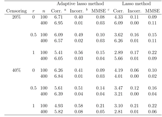
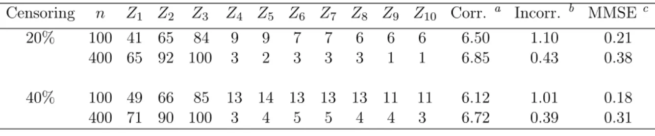
3.1 Average numbers of correct and incorrect zero coefficients and median mean square errors from
1000 simulated data sets . . . 45 3.2 Proportions of each covariate being selected and
signal-noise ratios for important covariates based on 1000 simulated data sets for the adaptive
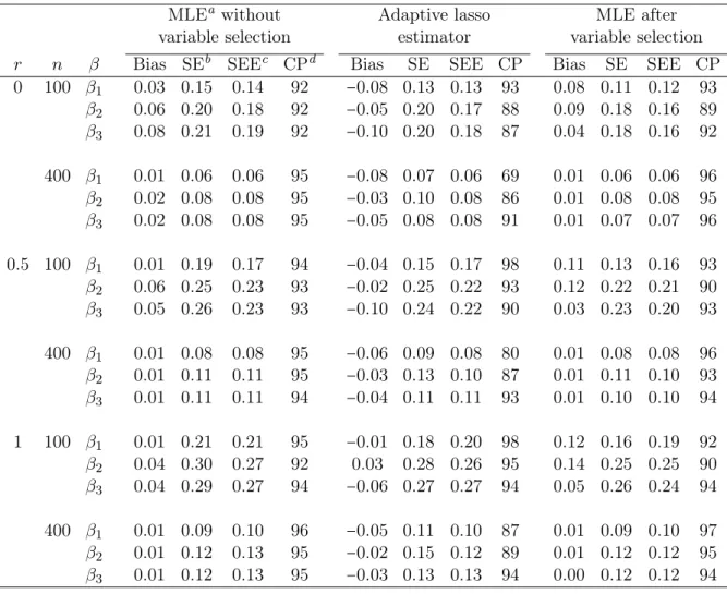
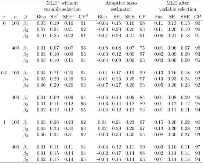
lasso method . . . 46 3.3 Estimates of coefficients, their standard errors,
and coverage probabilities for nominal 95% con-fidence intervals from 1000 simulated data sets
for censoring ratio 20% . . . 47 3.4 Estimates of coefficients, their standard errors,
and coverage probabilities for nominal 95% con-fidence intervals from 1000 simulated data sets
for censoring ratio 40% . . . 48 3.5 Variable selection proportions, average numbers
of correct and incorrect zero coefficients, and median mean squared errors from 1000 simu-lated data sets for the misspecified models using
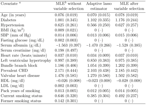
the adaptive lasso method . . . 49 3.6 Estimated coefficients and standard errors for
Atherosclerosis Risk in Communities data . . . 52 3.7 Estimated coefficients and standard errors for
primary biliary cirrhosis data under the
propor-tional odds model . . . 56 3.8 Estimated coefficients and standard errors for
primary biliary cirrhosis data under the
4.1 Comparison of three support vector learning meth-ods for right censored data using a linear kernel, with censoring times following the accelerated
failure time model. . . 78 4.2 Comparison of three support vector learning
meth-ods for right censored data using a linear kernel, with censoring times following the Cox
propor-tional hazards model . . . 79 4.3 Comparison of prediction capability for different
methods using Huntington’s disease data . . . 82 4.4 Normalized coefficient estimates using linear
ker-nel for Huntington’s disease data . . . 84 4.5 Comparison of prediction capability for different
methods using Atherosclerosis Risk in
Commu-nities data . . . 85 4.6 Normalized coefficient estimates using linear
ker-nel for Atherosclerosis Risk in Communities data . . . 87
5.1 Root mean square errors (RMSE) of compar-ing our method (GSVM) and Andersen and Gill proportional intensity model (AG) for the
pre-diction of recurrent events (Case 1) . . . 107 5.2 Root mean square errors (RMSE) of
compar-ing our method (GSVM) and Andersen and Gill proportional intensity model (AG) for the
pre-diction of recurrent events (Case 2) . . . 108 5.3 Root mean square errors (RMSE) of
compar-ing our method (GSVM) and Andersen and Gill proportional intensity model (AG) for the
pre-diction of recurrent events (Case 3) . . . 109 5.4 Root mean square errors (RMSE) of
compar-ing our method (GSVM) and Andersen and Gill proportional intensity model (AG) for the
5.5 Comparison of prediction capability for our method and Andersen and Gill proportional intensity
LIST OF FIGURES
2.1 (a) Estimation picture in two dimensions for the lasso (left) and ridge regression (right). Shown are contours of the objective and constraint func-tions. The solid areas are the constraint regions, while the ellipses are the contours of the least square objective function. (b) Contours of con-stant value of the constraint regions∑2j=1∣βj∣qfor
given values of q. . . 14 2.2 Plot of shrinkage functions withλ=2for (a) the
best-subset; (b) the bridge, q=0.5; (c) the lasso; (d) the bridge, q = 1.5; (e) the ridge; (f) the SCAD, a=3.7; (g) the adaptive lasso,γ =0.5; (h) the adaptive lasso, γ =2. The shrinkage func-tions are estimated under orthonormal regres-sion matrix by minimizing 1
2(β 0
j −βj)2+pλ(∣βj∣), where β0
j is the OLS estimate plotted on the
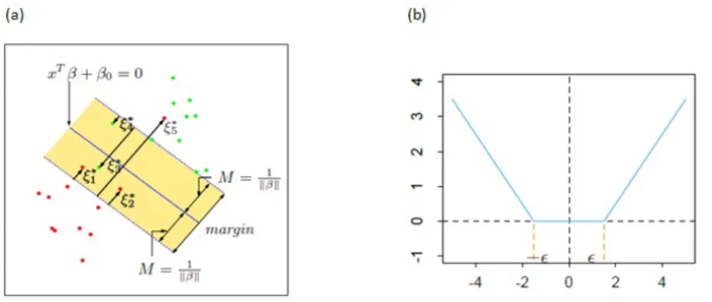
di-agonal. . . 16 2.3 (a) Nonseparable support vector machine for
clas-sification. (b) -insensitive error function used
by the support vector regression. . . 25 2.4 (a) Loss functions as defined by Shivaswamy et
al. (2007). (b) Loss functions as defined by
Khan and Zubek (2008). . . 30
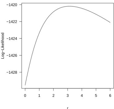
3.1 Fitted observed log-likelihood values for loga-rithmic transformation parameterrin the
Atheroscle-rosis Risk in Communities data. . . 51 3.2 Fitted observed log-likelihood values for
loga-rithmic transformation parameter r in the
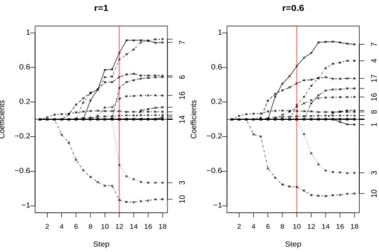
pri-mary biliary cirrhosis data. . . 55 3.3 Solution path for primary biliary cirrhosis data
4.1 Hazard Ratios comparing two groups separated using percentiles of predicted values as cut points for Huntington’s disease data. Dotted curve: Modified SVR; Dashed curve: IPCW-KM;
Dashed-dotted curve: IPCW-Cox; Black solid curve: SVHR. . . 83 4.2 Hazard Ratios comparing two groups separated
using percentiles of predicted values as cut points for Atherosclerosis Risk in Communities data. Dotted curve: Modified SVR; Dashed curve: IPCW-KM; Dashed-dotted curve: IPCW-Cox; Black
CHAPTER1: INTRODUCTION
Statistical model building is a challenging task for censored data when there are a large number of concomitant covariates. Existing methods tend to make strong assump-tions on the covariate effects or the censoring mechanism, making them unsuitable for the task of predicting future outcomes accurately. For example, the Cox proportional hazards model assumes that the hazard functions between two subjects are propor-tional over time. Although the model allows for time-varying covariates, it is apparent that the model excludes many complex covariate patterns. In this dissertation, we will develop statistical methods that are less dependent on the restrictive assumptions than the existing methods. Specifically, we generalize the efficient variable selection method to a class of transformation models; we adapt the popular support vector machines technique for statistical learning to the censored data that are represented by counting processes; also, we generalize this approach to recurrent event data.
1.1 Variable Selection in Semiparametric Transformation Models
and guaranteed to converge numerically. Under the regularity conditions in Zeng and Lin (2006), we show that our selection has oracle properties and that the estimator is semiparametrically efficient. We demonstrate the small-sample performance of the proposed method via simulations, and we use the method to analyze data from the Atherosclerosis Risk in Communities Study and Primary Biliary Cirrhosis Study.
1.2 Support Vector Hazard Regression for Predicting Survival Outcomes
1.3 Support Vector Machines for Predicting Recurrent Events
CHAPTER2: LITERATURE REVIEW
In this chapter, we review literature on statistical methods for semiparametric sur-vival models in Section 2.1, for traditional and penalized variable selection in Section 2.2, and for statistical supervised learning and outcome prediction in Section 2.3.
2.1 Semiparametric Models for Censored Data
In many medical trials, outcome of interest is survival time and is subject to censor-ing, where the exact survival time may be longer than the duration of the trial period and is therefore unknown. Typical examples include time to death from the start of a diagnosis, response time to a particular medical treatment, and time to recurrence of cancer tumor. It is often of interest to study whether certain clinical characteristics are related to occurrence of certain events and then examine the predictive values of sur-vival in terms of these covariates. Since the distributional assumption on the sursur-vival times is not valid in many situations, semiparametric methods are widely used.
The most popular semiparametric model for data fitting is the Cox (1972) propor-tional hazards model. Given the vector of covariates Z, this model is specified by a hazard function
one unit for the covariate in question. To efficiently estimate the regression coefficients, Cox (1972, 1975) introduced the partial likelihood principle to eliminate the infinite-dimensional baseline hazard function, and the resulting estimator was a function of the survival times only through their ranks. In the discussion of Cox’s paper (1972), Breslow (1972) proposed a nonparametric maximum likelihood estimator (NPMLE) for the arbitrary baseline hazard in (2.1) using the joint full likelihood and this estimator reduces to the Kaplan-Meier product limit estimator when there is no covariate effect. In a seminal paper, Andersen and Gill (1982) extended the Cox proportional hazard model to general counting processes to allow for recurrent event and established the asymptotic properties of the maximum partial likelihood estimator and the associated Breslow (1972) estimator of the cumulative baseline hazard function via the elegant counting-process martingale theory.
A concise alternative to capture the non-proportionality is the proportional odds model (Bennett, 1983a; 1983b). Under this model, the hazard ratio between two sets of covariate values converges to unity rather than staying constant as time increases. The survival function SZ, given the vector of covariates Z, is parameterized by
−log{
SZ(t)
1−SZ(t)
} =G(t) +βTZ (2.2)
whereGis an arbitrary baseline log-odds andβis a vector of regression coefficients. The nonparametric maximum likelihood estimation (NPMLE) for this model was proposed by Bennett (1983b). Bennett’s estimator ofβis the maximum profile likelihood estima-tor of β, with the baseline log-odds function being profiled out. Murphy et al. (1997) showed that this maximum profile likelihood estimator was consistent, asymptotically normal, and semiparametrically efficient. Further Murphy et al. (1997) demonstrated that the profile likelihood could be treated as a parametric likelihood and provided the asymptotic distribution for the profile likelihood ratio statistic. Another method to es-timateβ is maximizing the marginal likelihood of the ranks (Pettitt, 1983; 1984). Since this marginal likelihood cannot be calculated explicitly for all β, Pettitt (1983, 1984) used an approximation based on a Taylor expansion on the logarithm of the marginal likelihood atβ=0, however, the resulting estimator is biased and inconsistent. Lam and Leung (2001) employed the technique of importance sampling to express the marginal likelihood as an expectation with respect to some distribution. Their method is com-putationally intensive since the importance sampling is a Markov chain Monte Carlo (MCMC) algorithm. In addition, the theoretical properties of the maximum marginal likelihood estimator were not investigated.
covariates. This model can be written as
H(T) = −βTZ+ (2.3)
whereHis an unknown monotone transformation function,is a random variable with a known distribution and is independent ofZ, and β is a vector of unknown regression coefficients. If follows the extreme value distribution, model (2.3) becomes to the proportional hazards model, while if follows the standard logistic distribution, model (2.3) becomes to the proportional odds model. Several papers proposed general estima-tors for the regression coefficients. Dabrowska and Doksum (1988) provided estimaestima-tors in the two sample problem based on the marginal likelihood of ranks and the MCMC method. Their estimators suffer from severe bias under heavy censoring and the bias cannot be reduced by increasing the size of Monte Carlo simulation (Lam and Leung, 1997). Cheng et al. (1995) derived inference procedures from a class of generalized estimating equations based on dichotomous variables of pairwise ranks. They adjusted censoring by the inverse weight of the Kaplan-Meier estimator for the survival function of the censoring variable, so the validity of their procedures relies on the assumption that the censoring variable is independent of covariates. Chen et al. (2002) mentioned that such an assumption was often too restrictive, even for randomized clinical trials. Chen et al. (2002) proposed an estimator using martingale-based estimating equations and the estimating equations precisely become to the Cox partial likelihood score equa-tion for the proporequa-tional hazards model. Although all these methods established the consistency and asymptotic normality for their estimators, none of them is semipara-metrically efficient. In addition, the class of linear transformation models is confined to traditional survival (i.e., single-event) data and time-invariant covariates.
notation. LetN∗(t)be the counting process recording the number of events that have occurred by time t and Z(t) be a vector of possibly time-varying covariates. The cumulative intensity function forN∗
(t) conditional on Z(t) takes the form
ΛZ(t) =G{
ˆ t 0
Y∗
(t)eβ
TZ(s)
dΛ(s)} (2.4)
where G is a thrice continuously differentiable and strictly increasing function with G(0) = 0, G′(0) > 0 and G(∞) = ∞, Y∗(.) is a predictable process and Λ(.) is an un-specified increasing function, and β is a vector of unknown regression coefficients. For survival data, Y∗
(t) =I(T ≥t), where T is the survival time and I(.) is the indicator function; for recurrent event,Y∗
(.) =1. WhenN∗(.)has a single jump at survival time
T and covariates Z is time-invariant, model (2.4) reduces to the linear transformation model (2.3). Specifying the function G while leaving the function Λ unspecified is
Another important alternative to the Cox proportional hazard model is the accel-erated failure time model. This model provides a natural formulation of the effects of covariates on potentially censored response variable. Let T be the survival time andZ a corresponding vector of covariates. The model can be written as
logT = −βTZ+ (2.5)
where is a measurement error independent of Z andβ is a vector of unknown regres-sion coefficients. Note that model (2.5) does not belong to the linear transformation model, which has unknown H and known distribution of. Buckley and James (1979) proposed the least square estimator, where they used the least square normal equation and replaced a censored observation by its conditional mean based on the residuals and product limit estimator. Jin and Lin (2003) studied a broad class of rank-based monotone estimating functions, including the Gehan-type weight function and weighted log-rank estimating equation. Later Zeng and Lin (2007b) proposed an extension of model (2.5) to incorporate time-varying covariates, and the extended model no longer took the log-linear form. They used kernel smoothing to construct a smooth approxi-mation to the profile likelihood for the regression coefficients, and established that the resulting estimators were consistent, asymptotically normal, and semiparametrically efficient. They also provided an explicit estimator for the error distribution.
joint models of repeated measures and survival time in longitudinal studies. The non-parametric maximum likelihood estimators of all the proposed models were shown to be consistent, asymptotically normal and semiparametrically efficient via the modern empirical process theory. In their paper, Zeng and Lin (2007a) emphasized the flexible modeling capability and accurate prediction of semiparametric transformation models, and suggested using them in the practice of survival analysis.
2.2 Variable Selection for Censored Data
With the improvement of modern technologies in epidemiologic and genetic stud-ies, researchers are able to collecting many variables, such as patients’ characteristics, biomarkers and genotypes, to predict clinical outcomes. When a large number of vari-ables is included in prediction models it often causes over-fitting and results in low prediction power. On the other hand, it is commonly believed that only a few im-portant variables exhibit strong effects. Hence, it is desirable to identify those few important variables in the model building process. Prior knowledge from the scientific literature is formally seen as the most important rationale for including or excluding variables from a statistical analysis, which is not always available for all research ques-tions, and too often involves only the iterative imposition of exact (typically exclusion) restrictions on individual variables (Smith and Campbell, 1980; Walter and Tiemeier, 2009). Comparatively, data-driven variable selection is more flexible and as a result a commonly used method in practice.
2.2.1 Variable Selection Methods
if statistically significant, or by eliminating those that are not statistically significant, simultaneously adjusting for the other variables in the regression model. Despite the ease of implementation, disadvantages of stepwise selection are known from separate studies (Derksen and Keselman, 1992; Harrell et al., 1996; Steyerberg et al., 1999), including that arbitrary definitions of thresholds may lead to bias and overfitting; binary decisions about the inclusion of variables cause information to be lost; true predictors may be excluded in small data sets because of a lack of power; noise variables may be selected because of multiple comparisons problems; and that the solution may be only locally optimal. An alternative approach leading to the global optimal solution is the best-subset selection, which chooses a small subset of the predictor variables that yields the most accurate model when the regression is restricted to that subset. However, the best-subset selection is computationally infeasible when the number of predictors is large and extremely unstable since it is a discrete process where variables are either retained or dropped from the model (Breiman, 1996). Moreover, many variable selection approaches in use, such as stepwise selection and best-subset selection, make inferences as if a model is known to be true when it has, in fact, been selected from the same data to be used for estimation purposes. Ignoring the model uncertainty causes non-trivial biases in coefficient estimates and underestimation of the variability of estimated coefficients in the resulting model (Chatfield, 1995; Harrell et al., 1996; Steyerberg et al., 1999).
β= (β0, . . . , βd)T minimize a penalized residual sum of squares,
N
∑
i=1
(yi−β0−
d
∑
j=1
xijβj)2+λ
d
∑
j=1
p(∣βj∣), (2.6)
where (xi1, . . . , xid), i=1, . . . , N are predictor variables, yi, i=1, . . . , N are responses,
structure of the bridge estimators. In these algorithms, the tuning parameter λ needs to be searched over a grid of values using some criteria, such as cross-validation, gener-alized cross-validation (Craven and Wahba, 1979), Akaike information criterion (AIC) (Akaike, 1974), and Bayesian information criterion (BIC) (Schwarz, 1978). Later, Efron et al. (2004) proposed an extremely efficient algorithm Least Angle Regression (LARS) for computing the entire lasso path, which was proved to be a one-dimensional path of prediction vectors growing piecewise linearly from the origin to the full least-squares solution.
Frank and Friedman (1993), and Fu (1998) considered a more general class of re-gression estimators that minimized function (2.6) with bridge penaltyp(∣βj∣) = ∣βj∣q for
Figure 2.1: (a) Estimation picture in two dimensions for the lasso (left) and ridge regression (right). Shown are contours of the objective and constraint functions. The solid areas are the constraint regions, while the ellipses are the contours of the least square objective function. (b) Contours of constant value of the constraint regions ∑2j=1∣βj∣q for given values of q.
perform well.
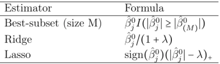
Table 2.1: Estimator ofβj in the case of orthornormal regression matrix. M and λ are constants chosen by the corresponding technique; sign denotes the sign of its arguments (±) and x+ denotes ”positive part” of x.
Estimator Formula
Best-subset (size M) βˆ0 jI(∣βˆ
0 j∣ ≥ ∣βˆ
0 (M)∣)
Ridge βˆ0
j/(1+λ)
Lasso sign(βˆj0)(∣βˆj0∣ −λ)+
solution in this family is lasso (q =1), but this comes at the price of shifting the re-sulting estimator by a constant λ. Furthermore, Fan and Li (2001, 2002) introduced the concept of oracle properties, that is, with appropriate choice of the regularization parameter, the true regression coefficients that are zero are automatically estimated as zero, and the remaining coefficients are estimated as well as if the correct submodel were known in advance. Knight and Fu (2000) showed that the bridge estimator with
0 < q < 1 possessed the oracle properties. Zou (2006) proved that the lasso (q = 1) could not be an oracle procedure, except in some simple settings such as orthonormal regression matrix or only two predictor variables, otherwise, a nontrivial condition was required for the underlying model to make the lasso selection consistent.
To overcome the limitations of bridge penalties, Fan and Li (2001) proposed the smoothly clipped absolute deviation penalty (SCAD), defined by its first derivative,
p′
λ(βj) =λ{I(βj≤λ) +
(aλ−βj)+
(a−1)λ
I(βj >λ)}
for some a>2 and βj >0, with pλ(0) =0, where pλ(.) is the λp(∣.∣) in (1), j =1, . . . , d. From the Bayesian statistical point of view, they suggested using a=3.7. The SCAD improves the lasso via penalizing large coefficients equally (e.g., see Figure 2.2(f)), and as a result, it has all the precedingly discussed theoretical properties. However, the nonconvex form of SCAD penalty makes its optimization challenging in practice, and the solutions may suffer from numerical instability (Zhang and Lu, 2007). Later, Zou (2006) proposed a new version of the lasso, called the adaptive lasso, where adaptive weights are used for penalizing different coefficients in the lasso penalty, that is,p(∣βj∣) =
wj∣βj∣,j =1, . . . , d. The weights are data-dependent and in the form ofwj =1/∣βˆj∣γ with
(a) (b) (c) (d)
(e) (f) (g) (h)
Figure 2.2: Plot of shrinkage functions withλ=2for (a) the best-subset; (b) the bridge,
q =0.5; (c) the lasso; (d) the bridge, q =1.5; (e) the ridge; (f) the SCAD, a=3.7; (g) the adaptive lasso, γ =0.5; (h) the adaptive lasso, γ =2. The shrinkage functions are estimated under orthonormal regression matrix by minimizing 1
2(β 0
j −βj)2 +pλ(∣βj∣), whereβ0
j is the OLS estimate plotted on the diagonal.
sense is the same rationale behind the SCAD (e.g., see Figure 2.2(g)-(h)), and as a result, the adaptive lasso is also an oracle procedure with continuity. Computationally, the adaptive lasso is a convex penalty, so the optimization problem does not suffer from the multiple local minima issue. Moreover, it is essentially a lasso penalization method so that all the current efficient algorithms for solving the lasso can be used to compute the adaptive lasso estimates.
penalizes the L1 norm of both the coefficients and their successive differences, and the sparsity property applies to the number of sequences of identical nonzero coefficients. Later, Meinshausen (2006) proposed the relaxed lasso, which used the lasso to select the set of nonzero predictors, and then applied the lasso again, but using only the selected predictors from the first step. For data where there are a very large number of noise variables, the relaxed lasso has sparser estimates and much more accurate pre-dictions than lasso. Recently, Radchenko and James (2011) proposed a method that could adaptively adjust the level of shrinkage, not just on the final model coefficients, as used in the relaxed lasso, but also during the selection of potential candidate models. They call this method forward-lasso adaptive shrinkage, which incorporates both for-ward selection and lasso as special cases, and can work well in situations where neither forward selection nor lasso succeeds.
2.2.2 Application of Variable Selection Methods to Censored Data
Extending penalized variable selection to survival analysis presents a number of challenges because of the complicated data structure, and therefore receives much at-tention in the recent literature. For Cox proportional hazards model, the objective function is parametric partial likelihood, denoted byli(yi;δi;ziTβ), where the collected data (yi, δi, zi) are independent samples, yi is the minimum of the failure time and censoring time, and δi is the censoring indicator. A general form of penalized partial likelihood is
n
∑
i=1
li(yi;δi;ziTβ) −n
d
∑
j=1
pλ(∣βj∣).
For accelerated failure time model, Johnson (2008) explored the penalized weighted rank-based statistics and the penalized Buckley-James statistics. Both are challenging because of the discontinuity and non-monotone in the regression coefficients. Motivated by these, Johnson et al. (2008) established the general theory for a board class of penal-ized estimating functions. Suppose that U(β) ≡ (U1(β), . . . , Ud(β))T is an estimating function forβ based on a random sample of sizen. They mainly studied the situations where U(β) was not a score function or the derivative of any objective function. A penalized estimating function is defined as
UP(β) =U(β) −nqλ(∣β∣)sign(β),
whereqλ(∣β∣)are coefficient-dependent continuous functions, and the second term is the component-wise product ofqλand sign(β). With the commonly used SCAD or adaptive lasso penalty, the resulting estimators were shown to be root-n consistent and enjoy the oracle properties. Johnson (2009) further improved the approximate zero-crossing of penalized Buckley-James estimating function by using a one-step imputation and a principled initial value. The one-step estimator is an exact zero-crossing, and with lasso penalty, it reduces to Tibshirani’s lasso as the proportion of censored observations approaches zero.
(2.3), the marginal likelihood is represented as
Ln,M(β) =
ˆ
V(1)<...<V(K)
ˆ n
∏
i=1
{λ(V(ki)+β TZ
i)}δie−Λ(V(ki)+β TZ
i) K
∏
k=1 dV(k),
where V(k) = H(T(k)), T(1) < . . . < T(K) are ordered uncensored failure times in the sample, δi is the censoring indicator, Λ(x) is the cumulative hazard function of , and λ(x) = dΛ(x)/dx. Since the marginal likelihood does not have a closed form, they approximated the high dimensional integrals and implemented the procedure by the computationally intensive MCMC algorithm, and did not give corresponding large sample properties.
Later, Zhang et al. (2010) proposed a penalized estimating equation estimator for linear transformation models (2.3). The estimator was constructed based on the mar-tingale difference equation for the unknown transformation function and the marmar-tingale integral equation for regression coefficients as in Chen et al. (2002). To tackle the diffi-culties of infinite dimensional parameter H, Zhang et al. (2010) introduced the notion of the ’profiled’ score, which was computed by plugging in the solution H˜ using the
current estimate ofβ. Let Ni(t)and Yi(t)respectively denote the counting and at-risk process, and the ‘profile’ score is
Un(β) =
n
∑
i=1 ˆ τ
0
Zi[dNi(t) −Yi(t)dΛ{βTZi+H˜(t;β)}].
Then they usedUn and its variance estimate to construct a loss function as
Dn(β) =Un′(β)V˜n−1Un(β),
where the inverse variance V˜−1
achieve the sparse estimation, they finally proposed minimizing
Qn(β) =Dn(β) +n
d
∑
j=1
pλ(∣βj∣).
By adopting the adaptive lasso penalty, they proved the root-n consistency and oracle properties for the resulting estimator. However, their method has the following limita-tions: (i) the implementation needs to solve the nuisance parameters by iteration; (ii) the resulting adaptive lasso estimator is not asymptotically efficient.
Recently, Li and Gu (2012) extended the approach of penalized marginal likelihood of ranks (Lu and Zhang, 2007) to a class of general transformation models with the form of
SZ(t) =Φ(S0(t), Z, β),
where SZ(t) is the conditional survival function of failure time T given covariate vec-tor Z; S0(t) is a completely unspecified baseline survival function; Φ(u, v, w) is a known monotonically increasing function with respect to u satisfying Φ(0, v, w) = 0 and Φ(0, v, w) = 1 for any v and w. Denote kn as the total number of uncensored failure times, R∗
n as the partial ranking among the kn uncensored failure times and the specified observations between each pair of uncensored observations, andLir as the
set of labels corresponding to those observations censored in interval [Tir, Tir+1). The rank-based marginal likelihood function is defined by
Ln(β) =Pr(Tn∈Cn∣R∗n, Z) =
ˆ
t∈Cn
(−1)n
n
∏
i=1
φ(S0(ti), Zi, β)
n
∏
i=1
dS0(ti),
where Cn = {(t1, . . . , tn) ∶ ti1 < . . . < tikn, tj ≥ tir, for j ∈ Lir and 0 ≤ r ≤ kn} and
was shown to be root-n consistent and satisfy oracle properties. However, their imple-mentation is still based on the MCMC algorithm, which is computationally intensive. In addition, it is not clear whether time-varying covariates can be included. Therefore, the current methods for variable selection in transformation models still leave a lot to be desired.
2.3 Statistical Learning for Censored Data
The science of learning plays a key role in the fields of statistics, data mining and artificial intelligence. In a typical scenario, we have a training set of data in which we observe the outcome and feature measurement for a set of objects. The goal is to build a prediction model, or learner, which will enable us to predict the outcome for new unseen objects. This is called supervised learning because of the presence of the outcome variable to guide the learning process and a good learner is one that accurately predicts such an outcome. A review of some popular supervised learning methods (Hastie et al., 2009) and their applications to censored data is given below.
2.3.1 Supervised Learning Methods
In supervised learning we seek a function f(X) for predicting Y given values of the input X. We also need a loss function L(Y, f(X)) for penalizing errors in pre-diction. For particular data sets, our goal is to find a useful approximation fˆ(x) to
kind of regular behavior in small neighborhoods of the input space. The larger the size of the neighborhood, the stronger the constraint, and the more sensitive the solution is to the particular choice of constraint.
The linear modelf(x) =xTβ makes stringent assumptions about the structure and yields stable but possibly inaccurate predictions. It relies heavily on the assumption that a linear decision boundary is appropriate. Comparatively, the method ofk-nearest neighbors is essentially model-free and assumesf(x) is well approximated by a locally constant function. The resulting prediction is often accurate but can be unstable. These two simple procedures are the basis for a large subset of popular techniques, such as kernel smoothing, basis expansions, generalized additive model, projection pursuit re-gression (PPR) model, neural network and so forth. Neural network is a two-stage regression or classification model, typically represented by a network diagram. Inter-pretation of the fitted model is usually difficult, because each input enters into the model in a complex and multifaceted way. As a result, it is most useful for prediction, but not very useful for producing an understandable model for data.
large tree is pruned using cost complexity pruning.
One major problem with trees is their high variability, that is, often a small change in the data can result in a very different series of splits. Bagging is a technique for reducing the variance by fitting the same tree many times to bootstrap-sampled versions of the training data. Another popular ensemble method is random forest, which improves the variance reduction of bagging by reducing the correlation between the trees. This is achieved in the tree-growing process through random selection of the input variables as candidates for splitting. As in bagging, the bias of a random forest is the same as the bias of any of the individual sampled trees. Hence, the improvement in prediction obtained by bagging or random forests is solely a result of variance reduction.
Another popular learning machine is support vector machines (SVMs) that produce decision boundaries for classification. This method has been applied in many areas, such as financial time series forecasting, determination of the layered structure of the earth, identification of human genes, content based image retrieval, intrusion detection of computer networks and so forth (Tay and Cao, 2001; Hidalgo et al., 2003; Fernandez and Miranda-Saavedra, 2012; Rao et al., 2010; Ganapathy et al., 2012). SVMs differ radically from comparable approaches such as neural networks, since their training always finds a global minimum and their simple geometric interpretation provides fertile ground for further investigation (Burges, 1998). Suppose that the training data consist ofN pairs(xi, yi),i=1, . . . , N, withyi∈ {−1,1}, and define a hyperplane by{x∶f(x) =
xTβ+β
0=0}, then a classification rule induced by f(x)is sign[xTβ+β0]. The goal is to find the hyperplane that explicitly tries to separate the data into different classes1
overlap in the training data (Figure 2.3(a)). This concept is captured by
min
β,β0
1 2∥β∥
2
+C
N
∑
i=1 ζi
subject to ζi ≥0, yi(xTi β+β0) ≥1−ζi,∀i
where the value ζi is the proportional amount by which the prediction f(xi) is on the wrong side of its margin and misclassifications occur when ζi > 1; the parameter
C is ’cost’ parameter and the separable case corresponds to C = ∞. This is a convex quadratic programming problem, since the objective function is itself convex, and those points which satisfy the constraints also form a convex set. This problem can be converted to its dual form by differentiating the corresponding Lagrangian function with respect toβ,β0 andζi, solving the results, and substituting the expressions back, and the dual objective function is
LD = N
∑
i=1 αi−
1 2
N
∑
i=1 N
∑
i′=1
αiαi′yiyi′xT
i xi′,
where αis are non-negative parameters. In this formulation, the training data will only appear in the form of inner products between vectors, so xT
ixi can be replaced by a kernel function K(xi, xi′) = ⟨h(xi), h(xi′)⟩to map data into a richer feature space
including non-linear features and allows SVMs to form nonlinear boundaries. The transformationhneeds not be specified at all and only knowledge of the kernel function is required. In the solution of this problem, those points for which αi > 0 are called support vectors, which lie closest to the decision hyperplance, are most difficult to classify, and would change the position of the decision hyperplane if removed.
Figure 2.3: (a) Nonseparable support vector machine for classification. (b)-insensitive error function used by the support vector regression.
written as a penalization method,
min
β,β0 N
∑
i=1
[1−yif(xi)]+ λ
2∥β∥
2 ,
2.3.2 Application of Supervised Learning Methods to Censored Data Many problems of medical prediction involve the use of right censored survival data, and censoring in the data is the main reason why standard supervised machine learning techniques are hard to use for modeling survival. Ripley and Ripley (2001) and Ripley et al. (2004) discussed and described models for survival analysis which is based on neural network. These models allow non-linear predictors to be fitted implicitly and the effect of the covariates to vary over time.
• In a discrete survival time context, most neural network survival methods are based on dividing up the survival time into discrete intervals, and estimating the probability of an event in each interval. With two intervals, survival is considered binary and this is an extension of logistic regression, where each censored patient is included twice, once as an event and once as a non-event. With more than two intervals, one way is to divide the survival time into one of a set of non-overlapping intervals, and view the outputs of the network as the absolute probability of an event in a particular interval. Another alternative is to model the conditional probability of an event given no events in the previous interval. Biganzoli et al. (1998) considered the feed forward neural networks with one input node assigned to each explanatory variable and an additional input for the time interval. This approach used entropy error function and could be easily implemented using software packages based on back-propagation.
model based on the input-output relationship associated with a simple feed for-ward network. They replaced the linear function βx in the partial likelihood by the output of the network and obtained the maximum likelihood estimates of the parameters of the neural network using the Newton-Raphson method.
Survival trees are popular nonparametric alternatives to (semi) parametric models. They offer great flexibility and can automatically detect certain types of interactions without the need to specify them beforehand (Bou-Hamad et al. 2011). In recent years considerable research effort has been dedicated toward extending classical trees to the case of censored data. These researches focused on utilizing different splitting and prun-ing criteria to involve survival time and censorprun-ing information. Segal (1988) replaced the conventional splitting rules with rules based on the Tarone-Ware or Harrington-Fleming classes of two-sample statistics, which measured the between-node separation instead of the within-node homogeneity. Leblanc and Crowley (1993) further general-ized Segal’s method by introducing a new algorithm that automatically chose the size of a tree and gave optimally pruned subtrees. They defined a measure of tree per-formance analogous to the cost complexity of CART for recursive partitions based on two-sample statistics and called it split complexity. Alternatively, Leblanc and Crow-ley (1992) proposed a tree-structured method that adopted the proportional hazards model and gave the relative risk estimates for censored survival data. In particular, the splitting criterion was based on a node deviance measure between a saturated model log-likelihood and a maximized log-likelihood, which was a measure of within-node er-ror. The advantage of this method is that it can be implemented easily in any recursive partitioning software for Poisson trees (Bou-Hamad et al. 2011).
2011). Hothorn et al. (2004) improved predicted survival probability functions of cen-sored event free survival by bagging survival trees. They computed a set a of survival trees based on bootstrap samples using the Leblanc and Crowley (1992) method, and then defined the aggregated Meier curve of a new observation by the Kaplan-Meier curve of all observations identified by the leaves containing the new observation. Later, Ishwaran et al. (2008) introduced the random survival forests for right censored data. Specifically, using independent bootstrap samples, each tree was grown by ran-domly selecting a subset of variables at each node and then splitting the node using a survival criterion involving the survival time and the censoring status information, and a tree was considered fully grown when each terminal node had no fewer than certain amount of unique deaths. Besides the several papers discussed here, extensive research on tree-based methods for the analysis of survival data with censoring was published over the last 25 years, reviewed by Bou-Hamad et al. (2011). The authors also covered more complex models, more specialized methods, and more specific problems such as multivariate data, the use of time-varying covariates, and discrete-scale survival data.
The appeal of support vector approaches derives from the fact that they are easy to compute and they enable estimation under weak or no assumptions on the distribution. Different methods have been suggested to adapt the support vector learning to censored data. Shivaswamy et al. (2007) proposed a support vector technique for regression on censored targets by generalizing the -insensitive loss function (Figure 2.4(a)). They considered the data set including censored targets that have covariatesxiand are within open-end intervals (li, ui) with li <ui, i=1, . . . , n, and penalized only if the predicted valuef(xi) was more than ui or if it is less than li. Thus, they gave the loss function for this case by
When li = −∞ (left censored) or ui = +∞ (right censored), this loss function became one sided. Suppose thatf is linear, f(xi) =wTxi+b; the formulation proposed for the censored dataset is:
min
w,b,ζ,ζ∗ 1 2∥w∥
2
+C(∑
i∈U
ζi+ ∑
i∈L ζ∗
i) subject towTi xi+b−ui ≤ζi, ∀i∈U
li−wTi xi−b≤ζi∗, ∀i∈L
ζi≥0 ∀i∈U; ζi∗≥0 ∀i∈L,
whereL contains the indices of those samples whose targets have a finite lower bound while U contains the indices of those having a finite upper bound. This formulation was also shown to be equivalent to the support vector machine and the support vector regression by setting li and ui appropriately. For non-censored targets, the support vector regression was used in their method. However, this method penalized incorrect predictions for left (right) censored data only if the prediction is higher (lower) than the observed censoring time, and penalized incorrect predictions the same whether the prediction was higher or lower than the observed event time (Van Belle et al. 2011b). Later, Khan and Zubek (2008) proposed an asymmetric modification to the -insensitive loss function which allowed censored data to be processed and accounted for the differences between censored and event instances (Figure 2.4(b)). Their method provided different losses for events and censored data and for predictions higher and lower than the observed time, and correspondingly in the formulation used different costs C and slack variables ζ for different situations. As a result, the major drawback was the large number of parameters to be estimated.
Figure 2.4: (a) Loss functions as defined by Shivaswamy et al. (2007). (b) Loss functions as defined by Khan and Zubek (2008).
accounted as in the standard support vector regression method. To handle censored data, they adopted the concept of concordance index and added the ranking constraints for all comparable data pairs. A data pair is said to be comparable whenever the order of their observed times is known, such as two events, an event and a right censored instances for which the censoring time of the latter is later than the event time of the former, and so forth. They considered the data points (xi, yi, δi), i =1. . . . , n, where
xis are covariates,yis are observed times andδis are censoring indicators, and assumed that the observed times were ordered (yi < yj for i <j), then the ranking constraints for predicted values were defined by
f(xj) −f(xi) ≥1−ζij, ∀i<j,
to be
f(xi) −f(x˜j(i)) ≥1−ζi, ∀i,
where ˜j(i) was the data point comparable with data point i and with the largest yj
smaller thanyi. Also, their formulation included only the ranking constraints and was for the problems whose primary interests were in defining risk groups instead of pre-diction of survival times. To evaluate the performance of support vector approaches for survival data, Van Belle et al. (2011b) compared several models based on ranking constraints, based on regression constraints and based on both ranking and regression constraints, and their results indicated a significant better performance for models in-cluding regression constraints than models only based on ranking constraints. However, the prediction rules to obtain the event times in these methods are not clear, and none of the above intuitive methods has theoretical justification. For example, the rank-based methods may not fully use observed event information, and it is unclear whether Van Belle et al. (2011b) is valid if the censoring time depends on the subject’s covariates.
From another perspective, Park and Jeong (2011) proposed a technique called re-cursive support vector censored regression to make a direct prediction of survival time. Their approach replaced the censored observations by the corresponding Buckley-James estimates and conducted the estimation through a recursive procedure. It is compu-tationally intensive and the theoretical properties were not studied. Later, Goldberg and Kosorok (2012b) developed a unified support vector approach for right censored survival data, and the general methodology to estimation was applied for the truncated mean, median, quartiles, and for classification problems. The core idea was to use the inverse-probability-of-censoring weighting to correct the bias induced by censoring, that is,
L(z, Y(u), s) × δ
ˆ
where L(.) was the original loss function, δ was the censoring indictor and Gˆn was a generalized Kaplan-Meier estimator for the survival function G. As a result, in their method, a different loss function was defined for each data set and minimizing the empirical loss no longer consisted of minimizing a sum of independent and identically distributed observations. They also showed that the proposed method was well defined and measurable, and derived finite sample bounds on the deviation from the optimal risk. However, their method may suffer from severe bias when the censoring distribution is misspecified. Additionally, the weights used in inverse weighting can become large in some situations. As a result, the computation of this method becomes numerically unstable and even infeasible.
CHAPTER3: VARIABLE SELECTION IN SEMIPARAMETRIC TRANSFORMATION MODELS
3.1 Methodology
3.1.1 Transformation Models
We let Z(⋅) = {Z1(⋅), . . . , Zd(⋅)}T denote a vector of d-dimensional possibly time-varying covariates used for predicting survival outcome T. A general transformation model assumes that the cumulative hazard function ofT given Z(⋅) is
Λ{t∣Z(⋅)} =G{
ˆ t
0
eβTZ(s)dΛ(s)}, (3.1)
whereΛ(⋅)is a completely unspecified cumulative hazard function, andβ= (β1, . . . , βd)T is an unknown vector of regression coefficients. If all covariates are time-invariant, the above model is equivalent tolog Λ(T) = −βTZ+logG−1(−log0),where0 has a uniform distribution.
The transformation G is assumed to have the form G(x) = −log
´∞ 0 e
−xζφ(ζ)dζ, whereφ(ζ)is a known density function on [0,∞). A commonly used choice of φ(ζ)is the gamma density with unit mean and variance r. Then G(x) arises from a class of logarithmic transformations (Chen et al., 2002):
G(x) = ⎧ ⎪ ⎪ ⎪ ⎪ ⎨ ⎪ ⎪ ⎪ ⎪ ⎩
log(1+rx)/r, r>0,
x, r=0.
1,G(x) =log(1+x)results in the proportional odds model. This class of transformations is commonly used, although any transformation induced by some density φ(⋅) with support in[0,∞) is applicable.
Suppose a random sample of n subjects is chosen. Let Ti denote the failure time and Ci denote the censoring time of the ith subject, respectively. Define the ob-served time Yi =min(Ti, Ci) and the censoring indicator ∆i =I(Ti ≤Ci). Let Zi(⋅) = {Zi1(⋅), . . . , Zid(⋅)}T be the corresponding vector of time-varying covariates for the ith subject. Thus, the observed data consist of {Yi,∆i, Zi(⋅)}, for i = 1, . . . , n. Here we consider only external time-varying covariates, that is, the whole trajectory of Zi(⋅) is observable. Assume that Ti and Ci are conditionally independent given Zi(⋅), and the censoring mechanism is noninformative. Under the transformation model (3.1), the likelihood function for the observed data is
n
∏
i=1
[Λ′(Yi)eβ
TZ i(Yi)
G′
{
ˆ Yi
0
eβTZi(s)dΛ(s)}]
∆i
×exp[−G{
ˆ Yi
0
eβTZi(s)dΛ(s)}], (3.2)
where Λ′
(Yi) is the derivative of Λ at Yi. Expression (3.2) involves both β and the infinite dimensional parameter Λ, and may not be concave in these parameters. Also,
there is no partial likelihood function available due to the transformation G. Thus, directly applying the penalized methods in Fan and Li (2002) or Zhang and Lu (2007) for variable selection is no longer feasible.
To resolve this difficulty, we adopt the method proposed by Zeng and Lin (2007). The idea is to treat ζ as a latent variable, in which case model (3.1) is equivalent to the survival timeT with cumulative hazard function
Λ{t∣Z(⋅), ζ} =ζ
ˆ t 0
because
pr{T >t∣Z(⋅)} = E[pr{T >t∣Z(⋅), ζ} ∣Z(⋅)]
= E[exp{−ζ
ˆ t
0
eβTZ(s)dΛ(s)} ∣Z(⋅)]
=
ˆ ∞
0
exp{−ζ
ˆ t
0
eβTZ(s)dΛ(s)}φ(ζ)dζ
= exp[−G{
ˆ t 0
eβTZ(s)dΛ(s)}].
That is, conditional on the covariates Z(⋅) and the latent variable ζ, the survival time
T follows a Cox proportional hazards model with ζ missing. Thus, instead of working on the observed data for variable selection, we work on the complete data so that the method for variable selection in the Cox proportional hazards model may be used.
The expectation-maximization algorithm is used to fit model (3.3) based on com-plete data, {Yi,∆i, Zi(⋅), ζi} (i=1, . . . , n). In this setting, the likelihood function (3.2) becomes
n
∏
i=1
{ζiδΛ(Yi)eβ
TZ i(Yi)
}
∆i
×exp{−ζi
ˆ Yi
0
eβTZi(s)dΛ
(s)} ×φ(ζi),
where Λ′
(Yi) is replaced by δΛ(Yi), the jump size of Λ at Yi, in the nonparametric maximum likelihood estimation.
expected log-likelihood obtained in the expectation step, which is n ∑ i=1 ⎡ ⎢ ⎢ ⎢ ⎢ ⎣
∆i{logδΛ(Yi) +βTZi(Yi)} −E{ζi∣Y,∆, Z,β˜k, δΛ˜k(Y)} ∑ Yj≤Yi
eβTZi(Yj)
δΛ(Yj) ⎤ ⎥ ⎥ ⎥ ⎥ ⎦ . (3.4)
After convergence, we obtain the maximum likelihood estimates β˜ and δΛ˜(Yi) (i = 1, . . . , n). The algorithm is guaranteed to converge, since the objective function (3.4) in the maximization step is increased in each iteration, and is only unchanged at con-vergence.
3.1.2 Variable Selection
The objective function (3.4) takes a very similar form to the Cox log-likelihood function. Based on the maximum likelihood estimates, we compute the posterior ex-pectation E{ζi ∣ Y,∆, Z(⋅),β, δ˜ Λ˜(Y)}, denoted as the weight ˜ci (i =1, . . . , n). These weights are data-dependent. As given in the appendix of Zeng and Lin (2007),
˜
ci= ⎧ ⎪ ⎪ ⎪ ⎪ ⎪ ⎪ ⎨ ⎪ ⎪ ⎪ ⎪ ⎪ ⎪ ⎩ G′
{∑nj=1I(Yj ≤Yi)eβTZi(Yj)δΛ
(Yj)}, ∆i=0, −
G′′
{∑nj=1I(Yj≤Yi)eβT Zi(Yj)δΛ(Yj)} G′
{∑nj=1I(Yj≤Yi)eβT Zi (Yj)
δΛ(Yj)}
+G′{∑nj=1I(Yj ≤Yi)eβTZi(Yj)δΛ
(Yj)}, ∆i =1.
Given ci˜, we differentiate function (3.4) with respect to δΛ(Yi) and set it to be zero, giving
δΛ(Yi) =
∆i
∑nj=1I(Yj ≥Yi)˜cjeβTZj(Yi).
SubstitutingδΛ(Yi)back into function (3.4), we obtain a weighted version of the partial log-likelihood function,
ln(β) =
n
∑
i=1
∆i[βTZi(Yi) −log{
n
∑
j=1
I(Yj ≥Yi)˜cjeβ
TZ j(Yi)
}]. (3.5)
is the objective function in the maximization step of the expectation-maximization algorithm, which results in the efficient maximum likelihood estimator β˜if maximized
without penalties (Zeng and Lin, 2006, 2007). An important advantage of function (3.5) is its strict concavity, as shown in the appendix. For the Cox proportional hazards model, (3.5) reduces to the partial likelihood function. These properties enable us to adopt similar procedures for the implementation to those for the Cox model, and to derive nice theoretical results for the estimator after variable selection.
Although many penalties can be applied with function (3.5), here we use the convex adaptive lasso penalty for computational simplicity. This penalty adapts each coeffi-cient with a weight to reflect the importance of the corresponding covariate, which is equivalent to using different tuning parameters for different coefficients. The coeffi-cients of unimportant covariates are assigned larger weights so that they can be shrunk to zero more easily, leading to the oracle property (Zou, 2006). The reciprocal of any consistent estimatorβ can be used as the adapting weights; here we take the maximum likelihood estimator β˜. Writing β = (β
1, . . . , βd), the corresponding penalized objective function is
−ln(β) +λ
d
∑
j=1
∣βj∣/∣β˜j∣γ, (3.6) whereγ is a given positive constant.
To obtain the adaptive lasso estimates βˆ, we need to minimize function (3.6).
As-sume that the covariatesZij(⋅)are standardized so that∑ni=1Zij(⋅)/n=0and
∑ni=1Zij2(⋅)/n=1. We modify the computational algorithm of Zhang and Lu (2007) for the proportional hazards model. The strategy is to approximate the weighted partial likelihood function as an iterative least squares step using a Newton–Raphson up-date. Define the gradient vector∇l(β) = −∂ln(β)/∂β and the Hessian matrix ∇2l(β) =
Taylor expansion for−ln(β) has the form
1
2(W −Xβ)
T
(W−Xβ). (3.7)
Hence to minimize the original problem (3.6) for any fixed λ, we use the following procedure:
Step 1. Use the expectation-maximization algorithm to computeβ˜andδΛ˜(Yi), and then compute the weights ˜ci (i=1, . . . , n).
Step 2. Initialize by setting βˆ=β˜.
Step 3. Compute∇l, ∇2l,X and W based on the current values of βˆ.
Step 4. Use the modified shooting algorithm (Zhang and Lu, 2007) to minimize the function (3.7) plus the penalty λ∑dj=1∣βj∣/∣β˜j∣γ.
Step 5. Repeat Steps 3 and 4 until the convergence criterion is met.
The initialization in Step 2 reduces the number of iterations compared with setting
ˆ
β=0, sinceβ˜is already consistent. In addition, withβˆ=β˜in Step 2, the estimates from the one-step iteration are fairly close to those from iteration until convergence. The minimization in Step 3 is based on a quadratic least squares function, so the path-based algorithms in the least squares setting for solving the adaptive lasso can be applied to compute the whole solution path for the one-step estimates.
partition the data into V subsets with equal sizes. For a given λ, we must compute the coefficients using V −1 subsets and function (3.7) plus the adaptive lasso penalty using the V th subset V times, which is computationally much more complicated to implement than generalized cross validation. The simulation studies in Section 3.3 show that generalized cross validation works well for our models.
After variable selection, we suggest refitting model (3.3) to obtain the maximum likelihood estimates for the coefficients of selected covariates. As shown in the previous literature, although the adaptive lasso estimator is consistent, its finite sample bias can be non-negligible.
3.1.3 Standard Errors
Our method treats the transformation as missing latent variables, so the Louis formula (Louis, 1982) is used to obtain the standard errors for the maximum like-lihood estimates. The Louis formula computes the observed information within the expectation-maximization framework. To apply it, we need to consider both the de-sired parameterβ and the nuisance parameterΛ, whereΛis evaluated at each observed
time point. Denote all the parameters asθ= {β1, . . . , βd, δΛ(Y1), . . . , δΛ(Yn)}T and the log-likelihood using complete data asfi (i=1, . . . , n). Then the covariance matrix of θ is
(−
n
∑
i=1 E{∂
2fi(θ)
∂θ2 ∣Y,∆, Z(⋅)} − n
∑
i=1
E[{∂fi (θ)
∂θ } ⊗2
∣Y,∆, Z(⋅)] (3.8)
+
n
∑
i=1
[E{∂fi (θ)
∂θ ∣Y,∆, Z(⋅)}] ⊗2
)
−1 .
We also apply formula (3.8) to approximate the standard errors for the adaptive lasso estimates. Instead of plugging inβ˜andΛ˜, we plug in the adaptive lasso estimates
ˆ
the standard errors, we set those for zero estimates to be zero, assuming that the cor-responding covariates are unimportant. Compared with the sandwich formula used in Zhang and Lu (2007), formula (3.8) does not have the tuning parameter λ. Intuitively, the information of λ is carried by the adaptive lasso estimates, andλ is small in most cases. This method can work well since the adaptive lasso estimator is asymptotically efficient, and reaches the same efficiency bound as the maximum likelihood estimator. Correspondingly, this efficiency bound can be consistently estimated by the covariance matrix of the adaptive lasso estimates.
3.2 Theoretical Properties
In this section we provide asymptotic properties for our estimators. We consider the penalized objective function based on n samples: Qn(β) = ln(β) −nλn∑dj=1∣βj∣/∣β˜j∣γ. Denote the true values ofβ and Λbyβ0 and Λ0. We writeβ0 as(β10T, β20T)T, where β10 consists of all q non-zero components and β20 consists of the remaining zero compo-nents. Correspondingly, we have the adaptive lasso estimatorβˆ
n= (βˆ1nT ,βˆ2nT )T and the maximum likelihood estimator after variable selectionβnˇ = (βˇT
1n,0)T. Also, we write the time-varying covariates Z(⋅) as {Z1(⋅)T, Z2(⋅)T}T, where Z1(⋅) denotes the important covariates and Z2(⋅) denotes the unimportant covariates.
We require the following regularity conditions.
Condition 1. The function Λ0(t) is strictly increasing and continuously differen-tiable, and β0 lies in the interior of a compact set.
Condition 2. With probability one, Z(⋅) has bounded total variation in [0, τ]. In addition, if there exists a vector α and a deterministic function α0(t) such that
α0(t) +αTZ(t) =0 with probability one, thenα=0 and α0(t) =0.
Condition 4. lim supx→∞{G(m0x)}−1log{xsupy≤xG′(y)} = 0 for any positive con-stantm0.
The same conditions are used in Zeng and Lin (2006). No additional conditions are needed for the adaptive lasso estimator. Conditions 1 and 3 are standard in survival models. Condition 2 is equivalent to saying that the design matrix {1, Z(t)} is full rank with some positive probability for all t ∈ [0, τ], and is used to show the strict concavity of the objective functionln(β). Condition 4 specifies the tail behavior of the transformation functionG(x). It is easy to check that the logarithmic transformation satisfies this condition.
Under Conditions 1–4, we claim the asymptotic results for our estimators.
Theorem 3.2.1. If n1/2λ
n = Op(1), then the adaptive lasso estimator satisfies ∥βˆn−
β0∥ =Op(n−1/2), where ∥ ⋅ ∥ denotes the Euclidean norm.
Theorem 3.2.2. If n1/2λ
n → 0 and n(γ+1)/2λn → ∞, then under Theorem 3.2.1, the
adaptive lasso estimator βˆn satisfies the following: (i) β2nˆ =0 with probability tending to 1;
(ii) n1/2(βˆ
1n−β10) =n1/2(Pn−P)Sβ1{Y,∆, Z1(⋅), β10,Λ0} +op(1), where Pn is the
empirical measure, with P being the expectation, Sβ1 is the efficient influence function for β1 as given implicitly in Zeng and Lin (2006), and op(1) denotes the random
el-ement converging to zero in probability in the metric space Rq. Consequently, βˆ 1n is semiparametrically efficient.
Theorem 3.2.3. The maximum likelihood estimator after variable selection β1nˇ satis-fies n1/2(βˇ
1n−β10) =n1/2(Pn−P)Sβ1{Y,∆, Z1(⋅), β10,Λ0} +op(1).
addi-due to the fact that the weighted partial likelihood function (3.5) is the objective func-tion in the last maximizafunc-tion step of the expectafunc-tion-maximizafunc-tion algorithm, so its maximizer without penalization is exactly the original maximum likelihood estimator. The additional penalization is not dominating, so it should not affect the asymptotic efficiency except by producing sparse estimation. Theorem 3.2.3 gives the theoretical properties for the maximum likelihood estimator of selected important variables after refitting the model without the adaptive lasso penalty after variable selection. Theo-rem 3.2.3 is from Zeng and Lin (2006). Proofs of TheoTheo-rems 3.2.1 and 3.2.2 are given in the Appendix.
3.3 Simulation Studies
3.3.1 Simulation Setup
Consider the logarithmic transformation for G. We consider three transformation models with r = 0, r = 0.5 and r = 1, where r = 0 yields the proportional hazards model and r = 1 yields the proportional odds model. We take ten covariates in the regression model, with true β = (0.3,0.5,0.7,0,0,0,0,0,0,0)T, so only the first three covariates have non-zero effects. The associated ten covariates Z = (Z1, . . . , Z10) are marginally standard normal with pairwise correlation corr(Zj, Zk) = ρ∣j−k∣, where ρ =
0.5. The failure times T are generated from the transformation model (3.1). The Weibull distribution is assumed for the baseline cumulative hazard function, withΛ(t) =