GST: GPU-decodable Supercompressed Textures
Pavel Krajcevski∗1, Srihari Pratapa†1and Dinesh Manocha‡1
1The University of North Carolina at Chapel Hill
http://gamma.cs.unc.edu/GST/
Disk
CPU
GPU
Image Compression (JPEG, PNG, WebP, etc)
Texture Compression (DXT, ASTC, PVRTC, etc)
Variable Bit-rate Compression (Olano et al. '11)
Supercompressed Textures with CPU decoder (Crunch, Wennersten and Ström '11)
Uncompressed: ~19MB 3584 x 1792
Supercompressed Textures with GPU decoder
(GST)
Compressed Image: ~800 KB Compressed Texture: ~4MB
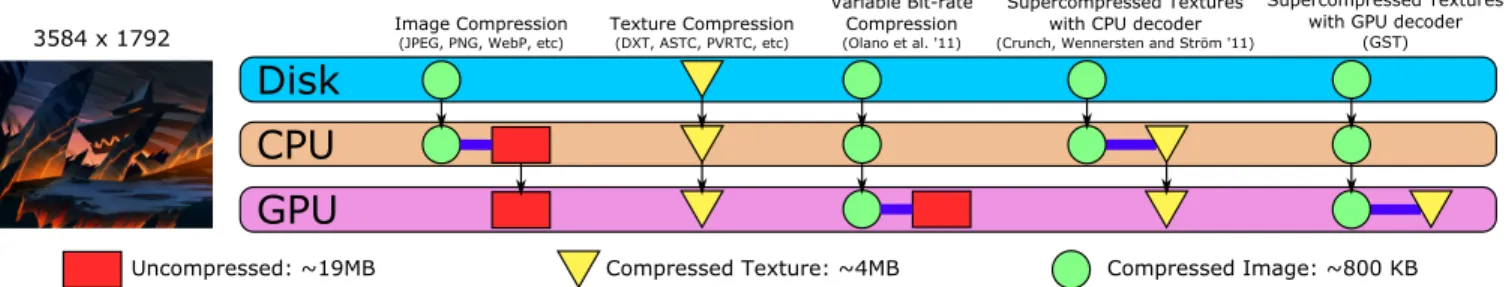
Figure 1: An overview of the methods for sending texture data from the disk to the GPU. Each vertical arrow indicates data sent over a bandwidth-limited channel. Each horizontal bar represents a decoding procedure. Green circles represent entropy-encoded data used for storage and streaming. Yellow triangles represent compressed texture data for use with hardware decoders in commodity GPUs. Red boxes represent the full uncompressed image data. We present a new method (GST) for maintaining a compressed format across all bandwidth-limited channels that decodes directly into a compressed texture on the GPU. Compared to prior techniques, our approach has the lowest CPU-GPU bandwidth requirements while maintaining compressed textures in GPU memory. Texture courtesy of Trinket Studios.
Abstract
Modern GPUs supporting compressed textures allow interactive ap-plication developers to save scarce GPU resources such as VRAM and bandwidth. Compressed textures use fixed compression ratios whose lossy representations are significantly poorer quality than traditional image compression formats such as JPEG. We present a new method in the class ofsupercompressedtextures that provides an additional layer of compression to already compressed textures. Our texture representation is designed for endpoint compressed for-mats such as DXT and PVRTC and decoding on commodity GPUs. We apply our algorithm to commonly used formats by separating their representation into two parts that are processed independently and then entropy encoded. Our method preserves the CPU-GPU bandwidth during the decoding phase and exploits the parallelism of GPUs to provide up to 3X faster decode compared to prior tex-ture supercompression algorithms. Along with the gains in decod-ing speed, our method maintains both the compression size and quality of current state of the art texture representations.
Keywords: texture compression, image compression, GPGPU
Concepts:•Computing methodologies→Image compression;
Graphics processors; Graphics file formats;
∗[email protected] †[email protected] ‡[email protected]
Permission to make digital or hard copies of all or part of this work for per-sonal or classroom use is granted without fee provided that copies are not made or distributed for profit or commercial advantage and that copies bear this notice and the full citation on the first page. Copyrights for components of this work owned by others than the author(s) must be honored. Abstract-ing with credit is permitted. To copy otherwise, or republish, to post on servers or to redistribute to lists, requires prior specific permission and/or a fee. Request permissions from [email protected]. c2016 Copyright held by the owner/author(s). Publication rights licensed to ACM. SA ’16 Technical Papers,, December 05 - 08, 2016, Macao ISBN: 978-1-4503-4514-9/16/12
DOI: http://dx.doi.org/10.1145/2980179.2982439
1
Introduction
For over a decade, commodity graphics hardware has shipped with dedicated compressed texture decoding units. Classically, these units decode a fixed number of bits into a block of pixels of prede-termined dimension to use with the texture sampling pipeline. Stor-ing compressed textures with respect to these hardware capabilities reduces the amount of bandwidth needed to transfer a texture into dedicated video memory, and the compressed representation allows for significantly more texture data to reside on the GPU.
Hardware texture compression formats map nicely to GPU architec-tures by allowing random-access to texture data. However, random access requires the texture to be encoded using fixed compression rates. In contrast to image compression formats such as PNG and JPEG [1992], which provide up to 50:1 compression, GPU texture formats commonly provide lower quality for file sizes at 6:1 com-pression. As an example, a 4K video frame (19MB uncompressed) requires 345KB of storage as a JPEG, whereas the same video frame requires3.21MB as a pure DXT compressed texture. This discrepancy is largely due to random access hardware requirements preventing the use of variable-length encoding techniques that are used in image compression. The result is that application develop-ers must choose between optimizing their data for streaming and optimizing for run-time efficiency, as image compression formats such as JPEG decode into fully uncompressed textures in memory. This trade-off becomes even more troublesome for applications that stream their texture assets over a low-bandwidth channel such as network-enabled GIS applications (e.g., Google Maps) and video game streaming services [Pohl et al. 2014]. Additionally, large vir-tual environments that cannot store all of their rendering data in memory would significantly benefit from lower disk-to-VRAM la-tency in order to avoid noticable loading artifacts.
in preparation for an entropy encoding step, such as Huffman or arithmetic encoding providing an additional 2-3X compression to regain the advantage of compressed image sizes on disk. However, decoding the texture on the CPU eschews the main benefits of com-pressing textures: the gained bandwidth across the CPU-GPU bus. This bandwidth is even more important in mobile devices that have power constrained GPUs [Leskela et al. 2009].
In this paper, we present a new supercompression algorithm GST, pronounced jist, for decompressing textures on the GPU into hardware-compressed formats. Our three main contributions in-clude:
1. A new supercompressed texture representation for endpoint-compressed formats;
2. A method for encoding textures into this format;
3. A parallel decoding algorithm suitable for SIMD architectures such as GPUs.
The basis of our algorithm is a state-of-the-art entropy encoding technique known as ANS that allows multiple compression streams to be interleaved and decoded in parallel on the GPU [Giesen 2014]. We exploit the underlying structure of commonly used endpoint compression formats in a way that increases the internal redun-dancy of the texture data, allowing for efficient static context mod-eling for the entropy encoder. Our approach saves both streaming and CPU-GPU bandwidth by providing compressed texture data to be decompressed by the device that will use it. Furthermore, one of our main benefits is the increased decoding speed realized by using massively parallel architectures.
We target the class of endpoint compression formats as described in Section 2.3. We first re-encode the per-pixel palette indices from a compressed representation into per-block dictionary entries. To improve redundancy between successive index blocks, we store the differences in sequential dictionary entries, similar to differen-tial pulse-code modulation (DPCM). Next, we treat the separate palette-generating endpoints of each block as two low-resolution images for which we use a wavelet transform. Finally, both of these parts are written to disk using entropy encoding. Our current implementation rivals the state-of-the-art CPU codecs in compres-sion size and quality with up to 3X improvement in decomprescompres-sion speed. This translates to about a 2-3X improvement in compres-sion size over the original hardware-compressed formats, which is realized as additional gains in CPU-GPU bandwidth when the su-percompressed texture data is sent to the GPU to be decoded. Our algorithm is designed from the ground up to target current desktop and mobile GPU architectures, and we show benefits to loading 4K video frames and large numbers of textures.
The rest of this paper is organized as follows. Section 2 discusses prior work and provides context for the dichotomy between image and texture compression algorithms. Section 3 gives an overview of our compression pipeline. Section 4 describes details on parallel encoding while Section 5 discusses implementation details for spe-cific compressed formats. Results are described in Section 6, and a discussion of limitations and future work is covered in Section 7.
2
Background
Texture data bandwidth has been a major, well-studied issue for interactive graphics applications for decades. In the rest of this sec-tion, we give a brief overview of texture and image compression techniques.
2.1 Image Compression
Traditional image compression algorithms such as PNG and JPEG use a variable-rate entropy encoding step to allocate bits to pixels with respect to their amount of detail. In order to prepare an im-age for entropy encoding, the raw RGB data usually undergoes one or more transforms in order to increase the amount of redundancy in the data. For example, JPEG uses the discrete cosine transform to condense the information content of blocks of pixels [Wallace 1992], and its successor, JPEG-2000, uses an optionally lossless wavelet transform [Skodras et al. 2001]. Similarly, colors are usu-ally transformed into color spaces that collect psychovisual detail into a single channel in order to increase overall compression effi-ciency. One such example is the lossless conversion of 8-bit RGB to a colorspace such as YCoCg [Malvar et al. 2008].
The entropy encoding stage of image compression algorithms is usually an inherently serial procedure that is difficult to paral-lelize. Olano et al. [2011] address this problem by proposing a new variable-rate compression scheme in which a GPU range codec is used to decompress the images by decoding differences between mip-levels. The resulting full-resolution textures are stored uncom-pressed in GPU memory.
2.2 Entropy Encoding
Techniques such as Huffman [1952], arithmetic [1979], and ANS [2013] encoding are the basis for many image compression formats [Buccigrossi and Simoncelli 1999]. Although entropy de-coding algorithms are inherently serial due to their variable length output, we may use multiple encoders and decoders in parallel. Duda [2013] presented asymmetric numeral systems (ANS) that maintains an internal state consistent between the encoder and de-coder. This property allows multiple encoding streams to be in-terleaved into a single data stream. Giesen [2014] uses this prop-erty to demonstrate how to create data streams that can be decoded in parallel using single-instruction multiple-data (SIMD) architec-tures. We give an overview of the range variant of ANS encoding and its use in our method in Section 3.3.
2.3 Texture Compression
The random access properties of compressed textures imply a fixed-rate compression ratio regardless of texture detail. This requirement allows texture mapping hardware to quickly compute an address to the underlying texture data. Typically, fixed-rate compression for-mats representN ×M blocks of pixels in some fixed number of bits. One of the earliest such representations was introduced by Delp and Mitchell [1979] to provide a two bit-per-pixel (bpp) lossy interpretation of eight-bit grayscale images. Later, many graphics architectures were proposed using similar compressed texture rep-resentations [Torborg and Kajiya 1996; Knittel et al. 1996; Beers et al. 1996].
recreate the final pixel values. Fenney [2003] targeted the worst-case filtering step of DXT by providing a compression format that bilinearly interpolates palette data across block boundaries. Later, the BPTC specification and ASTC introduced many improvements upon the original DXT format that provide multiple palettes per block, variable precision palette indices, a variable number of in-dices per block, and even variable global block sizes [OpenGL 2010; Nystad et al. 2012].
The second class of texture compression formats is known astabled compression formats. These formats store a single color per block of N ×M pixels and per-pixel offsets. Str¨om and Akenine-M¨oller [2004; 2005] introduced the first tabled formats as PACK-MAN and iPACKPACK-MAN. Later, Str¨om and Pettersson [2007] im-proved upon iPACKMAN by exploiting unused encoded represen-tations to provide additional detail.
Although most texture hardware requires random-access to the pixel data, many architectures have been proposed to alleviate this constraint. Inada and McCool [2006] proposed texturing hardware that stores textures in a b-tree to allow for efficient pixel access. Similarly, Krajcevski et al. [2016] presented a scheme that provides variable bit-rate texture compression by adding a layer of indirec-tion to dynamically select ASTC block sizes for regions of an im-age.
2.4 Supercompressed Textures
In order to reduce the streaming latency of textures, most appli-cations store these compressed texture formats (e.g., DXT, ASTC, ETC) on disk without additional processing. Recently, however, there has been progress into targeting both on-disk compression and in-memory compression. Str¨om and Wennersten [2011] pro-posed a scheme for further compressing ETC2 textures. In their formulation, they predict the final pixel colors in order to predict the per-pixel indices for the given block. They observe a gain of up to 3X in some cases over existing ETC2 textures. A differ-ent approach, known asCrunch, developed by Geldreich [2012], uses a Huffman-encoded dictionary of endpoints and index blocks to further compress a DXT-encoded texture. Blocks are stored in order using the differences between successive dictionary entries. Both of these methods decode the compressed texture on the CPU before sending them to the GPU. In this paper, we present an ap-proach for supercompression that preserves bandwidth using GPU decompression similar to Olano et al. [2011], while maintaining the decompression benefits of DXT.
3
Compression Pipeline
In this section we present our encoding scheme and discuss the techniques used to prepare our data for entropy encoding. Our su-percompression algorithm is designed to be compatible with many widely used texture formats and to map well to current GPU archi-tectures. Our approach is based on fulfilling the following design goals:
• The supercompressed texture representation should be di-rectly decodable on SIMD architectures, such as GPUs, with-out additional processing.
• The final decoded result should be a compressed texture in GPU memory.
• The supercompressed texture representation should be agnos-tic to the underlying endpoint compression formats.
Given an endpoint compressed texture representation, our compres-sion pipeline is organized in three stages, one for each of the
con-Per-pixel Palette Indices
Endpoint One Endpoint Two
Endpoint One
Endpoint Two
Per-pixel palette indices
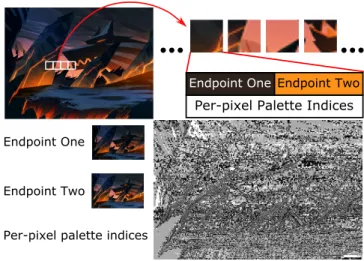
Figure 2: The constituent parts of a compressed texture. Each endpoint compressed texture represents a sequence of equally sized blocks. Each block contains a fixed number of bits containing two endpoint colors that generate a palette and per-pixel index data. Here we show the endpoints separated into individual images and visualize the per-pixel indices. We re-encode the indices using VQ-style dictionary compression and transform the endpoint images us-ing a wavelet transform prior to encodus-ing the final texture usus-ing an entropy encoder.
stituent parts of a compressed texture as described in Figure 2, and one for the final entropy encoding. Only the first stage introduces a minimal amount of error while the last two stages are lossless. In the first stage, starting with the original texture, we generate an ini-tial target endpoint compressed representation. We then re-encode each compressed block in an attempt to reuse indices from succes-sive blocks of pixels in preparation for dictionary encoding similar to vector quantization (VQ). In doing so, we also generate a new set of endpoints per-block. In the second stage, we independently pro-cess these endpoints as separate low-resolution images in prepara-tion for entropy encoding. Finally, we combine similar data streams and encode each using the range variant of ANS before storing to disk [Duda 2013]. The final output of our compression pipeline is four ANS streams to be decoded as described in Section 4.
3.1 Index Block Dictionary Generation
The per-pixel palette indices are classically the most difficult piece of information to compress [Str¨om and Wennersten 2011][Waveren 2006]. The first step in our compression pipeline is a re-encoding stage as described in Figure 3. The purpose of this step is to recom-pute palette indices for blocks of pixels in a way that is conducive to dictionary construction, similar to VQ. The endpoints for each block are then optimized to fit these newly assigned indices. Our goal is to build a dictionary ofindex blocksrepresentingN ×M blocks of indices. As an example, a4×4block of pixels that uses two-bit palette indices will have a dictionary of thirty-two bit index blocks. The goal of the dictionary is to have many redundancies in order to map well to the final entropy encoding step of pipeline as described in Section 3.3.
addi-Endpoint Format Encoder (DXT, PVRTC, etc)
Input
Palette Indices
Dictionary
Optimal
Re-encoder
Output Palette Indices
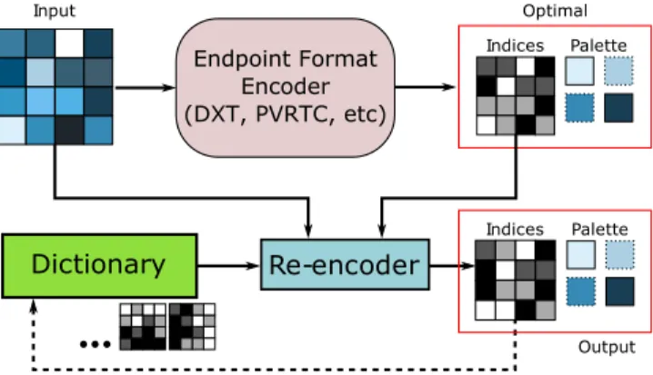
Figure 3: The first stage of our encoding pipeline. We process each block in raster-scan order while maintaining a dictionary of recently added index blocks. For each index block, if we find an existing index block in the dictionary that closely matches the orig-inal, we reuse that index block. If significant error is introduced, then we add this index block to the dictionary.
tional mean-squared error that can be introduced for a given block. Comparing against the original compressed representation, we pro-ceed by searching for recently added index blocks to the dictionary. If no such dictionary entry is found, then we add the index block corresponding to the original indices for that block to the dictionary. The amount of overall error introduced in the compressed represen-tation is directly related to the choice ofE. This error threshold is a simple way to affect the rate versus distortion properties of our com-pression method. By choosing a higher value forE, we get more redundancy in our dictionary, as more recently used index blocks become acceptable, but introduce additional error resulting in more noticeable compression artifacts.
Similarly to VQ, we replace each index block in the texture with a dictionary entry. In order to decrease the number of bits required to store the entries, we only consider the lastkdictionary entries. This allows us to represent a given block’s dictionary entry as a delta in the range[−k, k]from the previous block’s entry. The entries can then be reconstructed performing a prefix-sum. By increasing the size ofk, we have a smaller dictionary to store but suffer from the increased size of each dictionary entry. Although we process blocks in raster-scan order, different images may provide better delta com-pression using different orderings, such as a Z-curve. In our ex-periments, the compression performance of each ordering is highly dependent on the texture, and can be specified in a small per-file header. In our implementation, however, we choose raster-scan or-der andk = 127in order to represent each entry delta using one byte.
In order to determine the amount of error introduced by deviat-ing from the optimal index block, we use an optimization tech-nique for the endpoints found in many existing endpoint texture en-coders [Fenney 2003; Brown 2006; Casta˜no 2007; Krajcevski et al. 2013]. For endpoint-based texture compression each reconstructed pixel comes from a palette generated by two endpointspAandpB.
The number of palette entriespi is determined by the number of
bitsballotted to each pixel index in an index block,
pi=
(2b−1−i)pA+ipB
2b−1 ,
withi ∈ [0,2b−1]. Using this formulation, for a given index block we can construct aN M×2matrixBsuch that the optimal endpointspA andpB are found by minimizing the least-squares
error of the equation
B
pA
pB
−[px]
,
where eachpxcorresponds to the RGB value of thex-th pixel in
the original block.
3.2 Endpoint Processing
The second stage of our compression pipeline handles the endpoints themselves. Once the index block dictionary is generated, each block in the texture contains two RGB endpoints that define the palette for that block. Similarly to the PVRTC algorithm, we con-sider these endpoints independently as two separate low-resolution images that approximate the final image [Fenney 2003]. Each of these images can be treated independently as a separate image us-ing traditional compression techniques.
Our endpoint encoding step processes the images in two steps prior to entropy encoding, similar to JPEG2000 [Skodras et al. 2001]. The first step is a decorrelation step in order to improve the redun-dancy of neighboring values and to collect the visual information into a single channel. We chose the lossless YCoCg transform in order to avoid additional loss in the final texture and for its simplic-ity of implementation [Malvar et al. 2008]. The lossless property of this color transform is important because any additional error is magnified by the block dimensions in the final reconstructed im-age. The second step applies a wavelet transform to each color plane after the YCoCg transform. This step alters the total distri-bution of values in order to skew their probability distridistri-bution in preparation for entropy encoding. In our experiments, the choice of wavelet basis does not significantly affect the resulting compres-sion size. However, in order to preserve lossless comprescompres-sion of the endpoints, we use the CDF 5/3 wavelet as in JPEG2000 [Cohen et al. 1992].
3.3 ANS Entropy Encoding
The final stage of our compression pipeline combines the output of the two previous stages into a single data stream. Each previous stage produces two symbol streams with different probability dis-tributions requiring a separate context model for each. The index block dictionary and entries comprise the two streams from the first stage, and the second two are the separate Y and CoCg streams for the combined endpoints (Figure 4). Each of the four streams are en-tropy encoded separately and the results are concatenated and saved on disk along with the associated probability distributions. In the rest of this subsection we describe the entropy encoding technique used, known as Asymmetric Numeral Systems (ANS), first intro-duced by Duda [2013].
3.3.1 Background
Entropy encoding is a general term used for any method that con-verts a sequence of values, orsymbols, chosen from analphabet, into a sequence of bits based solely on the probability of each value appearing in the input stream. The earliest such method, known as Huffman coding, directly assigns a pattern of bits to each possible input symbol [Huffman 1952]. The length of each bit pattern cor-responds to the probability of that symbol appearing in the input stream. Compression occurs when the probability of a few symbols is far larger than the probability of others.
In Huffman encoding, since each symbol is represented byb ∈Z
non-power-of-two probability distributions (ormodels) of symbols used with the input sequence. To rectify this limitation, a tech-nique known as arithmetic coding takes a different approach [Ris-sanen and Langdon 1979]. Both encoder and decoder take as in-put an alphabet of symbolsA ={0, ..., n−1}with probabilities p0, ..., pn−1 such that1 =Pns=0−1ps. The encoder maintains two
values, orstates,LandH, that describe the range of numbers that encode all previously seen symbols. InitializingL= 0andH= 1, for each symbolsreceived as input, the encoder alters the states by the following formula:
Lnew=L+ (H−L) s−1 X
i=0
pi
Hnew=Lnew+ps(H−L)
The final result written to disk can be any number in the range [L, H). This number uniquely determines the input sequence for the given probability distribution of symbols inA. Compression occurs when the numbersLandHare relatively far apart, and we can choose a number that requires few bits to represent within that range. In particular, we can see that for a sequence of symbols s0, s1, ..., the rangeH−L gets smaller at the rate ofps0ps1....
This implies that the number of bits needed to represent a number in this range grows at the rateO(log 1
pi), which matches the
opti-mal theoretical limit established by Shannon [1948]. By knowing the final result, the decoder can follow the same procedure as the encoder and stop upon reaching the end of the bit stream.
3.3.2 Asymmetric Numeral Systems
ANS is similar to arithmetic encoding in that it approximates the theoretical limit to compression size, but has certain proper-ties that make it amenable for implementation on SIMD archi-tectures. The input to the compression algorithm is an alphabet
A={0, ..., n−1}, a stream of input symbolss∈ A, and a prob-ability distribution{ps},Psps = 1. Commonly, this probability
distribution is discretized with the approximationF:A →Nsuch
thatF(s)/M ≈ps, whereM =PsF(s). We use the common
approach of using the notationFsto representFs =F(s). Given
a symbolsand astatex ∈ Nthat encodes all of the previously
seen symbols of a given stream, ANS provides an encoderCand a decoderDsuch that
C(s, x) =x0 =M
x Fs
+Bs+ (xmodFs)
D(x0) = (s, x) =
L(R), Fs
x0 M
+R−Bs
,
where
R=x0modM and Bs= s−1 X
i=0
Fi.
The functionLis a lookup function that determines the symbols such that
L(z) = max
Bs<zs.
It follows thatCandDare direct inverses of each other, a property that arithmetic coding does not satisfy. Furthermore,CandDare monotonically increasing and decreasing with respect to the statex, respectively. The more interesting property is that our state grows at a rate similar to that of arithmetic encoding, requiringO(logM
Fs)≈ O(logp1
s)bits per symbol.
In order to stream data into and out of bits, as is required for use with a physical machine, each intermediate statexmust be normal-ized. In other words, we must write data to disk and decreasexin
order to prevent it from growing out of physical memory bounds, typically a 32-bit register. Duda [2013] claims that this is possible by defining a normalized interval[L, bL)such thatL =kM for somek, b∈N. In this interval,brepresents the divisor required to
normalize the interval. In the encoder,C, wheneverxgrows larger thanbL, thenxis repeatedly normalized byx/buntilx∈[L, bL). For each required normalization, the compressorCfirst writes the correspondingx(modb)to disk. Common choices forbare powers of two in order to map nicely to integer shift and bitwise masking operations during encoding and decoding. Just as the encoder may exceed the normalized interval from above, a decoder may require normalization whenx < L. In this case, the decoder will read a value of sizebfrom disk and increasexbyx0 =bxuntilxis in the normalized interval. In order to maintain reciprocity with the encoder, a decoder is required to read from disk at the same point in the data stream that the corresponding encoder wrote to disk. However, it is not required that the data for the data stream remain contiguous in memory, which is a separate property from arithmetic coding.
3.3.3 Preparing ANS for Parallel Decoding
As with all entropy encoding, the variability of the length of the re-sulting data stream makes it difficult for decoders to start working in parallel, or for a single decoder to be parallelized. In general, par-allel decoding approaches have required additional metadata to to the start positions in the datastream, increasing the overhead of the compressed data. ANS provides new properties for being amenable to GPU decoding. The biggest advantage that ANS gives is thatC andDare inverses of each other, as defined in Section 3.3.2, and always read or write a value of sizebto disk. As Giesen [2014] shows, if we haveNcompressorsCiworking in parallel, then all
Ncan operate in lockstep and share a common data stream as long as they write to disk in a deterministic ordering. To maintain the reciprocity between the corresponding set ofN decodersDi, we
must make sure that all decoders read from the shared stream in the same order that the encoders wrote to. This will ensure that each of the inputs to a given decoderDiwill be exactly the output from the
corresponding encoderCi.
Furthermore, if we choosebsuch thatb≥M, then we know that each encoding step will at most write one value in the range[0, b) to disk during state normalization. This property implies that each encoder will write at most one valuexmodbto disk per encoded symbol and hence each decoding thread (e.g. on a GPU) will read at most one such value per decoded symbol. Each state normalization therefore requires the evaluation of a conditional rather than a loop. A lock-step SIMD implementation such as those found in GPUs will always require each decoder to read at the same machine in-struction, and by masking out the threads that must read from disk, we can maintain the order of reads and decode in parallel. Using a value ofb= 2nwe ensure an integer number of bits being
written and read from disk. Once all encodersCifinish writing to
the shared stream,Nfinal encoding statesxiwill be used to seed
the decoders during decompression. We discuss these trade-offs in more detail in Section 4. To map well to current GPU architectures, the rest of this paper will assume the settingsk = 22, b = 216, M = 211, and|A|= 28.
4
Parallel Decoding
Data Stream
Symbol Frequencies
Y planes ANS Stream
CoCg planes ANS Stream
Index Dictionary ANS Stream
Dictionary Entries ANS Stream
ANS Table Builder
ANS Table
ANS Table
ANS Table
ANS Table ANS Decoder
Endpoint 1
Y Plane Endpoint 2Y Plane Endpoint 1Co Plane Endpoint 1Cg Plane Endpoint 2Co Plane Endpoint 2Cg Plane DictionaryIndex Entry DeltasDictionary
Inverse Wavelet Transform Parallel Scan
Endpoint 1 Endpoint 2 Dictionary Entries
Compressed Texture Assembler
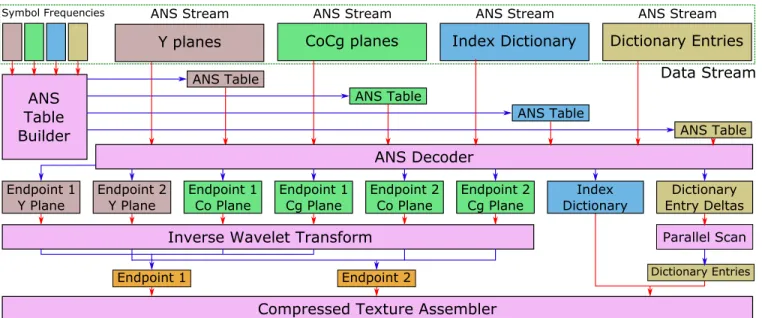
Figure 4: Our decompression pipeline. Pink boxes represent separate GPGPU executions for which red arrows are inputs and the blue arrows are the outputs. Per our design, the supercompressed texture data can be uploaded directly to the GPU for decoding. The input data and intermediate results all remain resident in GPU memory during decoding. Multiple texture streams can be interleaved between the symbol frequencies and the ANS streams to provide additional decoding parallelism.
commodity GPUs, but our algorithm can be appropriated to any SIMD architecture. In practice, the main trade-off of our method is between decompression speed and compression size. Our com-pressed representation contains a small header in order to properly construct the data pointers needed to begin the decoding process on the GPU. For a full implementation of both CPU encoder with GPU decoder, please refer to the source code included as supplementary material.
ANS is able to take advantage of SIMD hardware by interleaving many compression streams and decoding them in parallel. One of the biggest constraints is the number of streams that can be leaved at a time. In order to determine the order in which the inter-leaved compressors read from the shared compression stream, each decoder thread must notify all the others that it is reading in order to advance their shared offset [Giesen 2014]. Although arbitrarily many encoders can be interleaved, we suggest using 32 or 64 in order to use the available 32-bit or 64-bit shared registers that map well to the warp size of certain GPU vendors.
Additionally, the number of symbols encoded per thread has signif-icant implications on the decoding performance and compression size. First, each decoding thread must be initialized with the ANS state of the corresponding encoding stream. The fewer symbols en-coded per thread will increase the total number of threads and hence will also increase the storage overhead of the encoder states. How-ever, decreasing the total number of encoded symbols per thread increases overall parallelism by giving the GPU additional oppor-tunity for scheduling work while waiting on reads and writes to global memory. Finally, the total number of symbols encoded per thread limits the resolution of the final texture. In our method, we use a fixed number of symbols per encoding stream in order to keep all threads busy during decoding. Due to each endpoint belonging to a block of pixels, the number of symbols per set of encoders must divide the total number of pixel blocks in the texture. In our approach, we choose to use256symbols per thread requiring the total number of pixel blocks to be a multiple of256×32 = 8192. The ramifications of these trade-offs are shown in Figure 5.
Each ANS decoder relies on a context model given by the frequen-ciesFsdescribed in Section 3.3. The decoder needs to know the
values ofFs and Bs along with a fast implementation ofL(z).
Hence, each ANS encoded stream contains an additional set of fre-quenciesFson disk. Because we knowz ∈ [0, M), we can
con-struct a table of sizeM containing triplets(s, Fs, Bs) for every
possiblez. This table can be constructed from the set ofFsas a
parallel prefix-sum to construct theBsand a parallel binary search
to findsfor each value ofz. Constructing this table is the first step of our parallel decoding process as outlined in Figure 4. Using this table across all decoders requires us to use static histograms as our probability distribution. Adaptive models are difficult to implement because of race conditions while updating the model from different threads.
5
Implementation
Many of the limits of SIMD architectures require careful consid-eration of implementation details. Our method mainly focuses on further encodingendpointcompression formats as described in Sec-tion 2.3. We present an investigaSec-tion of the compression pipeline presented in Section 3 with respect to the DXT and PVRTC com-pression formats. We have chosen these formats due to their sim-plicity and widespread usage [Iourcha et al. 1999][Fenney 2003]. PVRTC and DXT differ only in the amount of bits allotted to store the endpoints and the manner in which their corresponding hard-ware reconstructs the compressed block. The compression quality of the texture is largely determined by the target hardware com-pressed format, although DXT and PVRTC usually provide similar quality encodings.
5.1 DXT
additional index blocks (DXT5) [Iourcha et al. 1999].
DXT1 has two palette generation modes depending on which order the RGB endpoints are placed. If the 16-bit integer representation of the first endpoint yields a smaller value than the second end-point, then only three palette colors are generated and the fourth corresponds to a solid black or transparent pixel. The optimal end-point values described in Section 3.1 for a given DXT index block may be generated in either order. In the case in which these end-points do not generate the expected four-color palette, we discard the index block as invalid.
During the color transform step as described in Section 3.2, we at-tempt to maintain the low bit depth of the pixel channels. Maintain-ing a low bit depth allows us to limit the number of symbols needed for entropy encoding following the wavelet transform. In the case of DXT1, endpoints are stored using five, six, and five bits for the red, green, and blue channels, respectively. Each565RGB value can be losslessly converted to667YCoCg [Malvar et al. 2008]. Af-ter performing the wavelet transform on each channel of the YCoCg data separately, we need less than eight bits to represent the coef-ficients. In order to increase parallelism, we use32×32blocks of endpoints. As this wavelet transform is operating on endpoints per4×4pixel blocks, this implies that we currently limit the di-mensions of each texture to be a multiple of128. This block size was chosen to map well to the common limit of 256 threads per work-group on modern AMD GPUs.
5.2 PVRTC
PVRTC is similar to DXT in that it has the ability to choose between opaque and transparent textures in the compressed block represen-tation. However, in the original PVRTC, the opacity of the color is determined on a per-endpoint basis rather than on a per-block basis. As a result, each color contains an extra bit to determine whether or not the color contains opaque RGB values or transparent RGBA values. A further bit is provided to alter the generated palette to provide a similar punch-through alpha as in DXT1. In contrast to DXT, these features of PVRTC are agnostic to the ordering of the endpoints, so we can choose opaque endpoints every time to match the generated endpoints from the re-encoding described in Section 3.1 [Fenney 2003].
Additionally, PVRTC uses lower-precision endpoints than DXT1. Where DXT1 stores three-channel endpoints with 565 precision, PVRTC stores endpoints using 555 and 554 precision. With 565 endpoints, the additional bit in the green channel requires addi-tional bits in the resulting YCoCg transform. However, using 555 endpoints restricts the additional bits needed for YCoCg to an addi-tional bit in the Co and Cg channels, meaning these endpoints can be represented using 566 YCoCg, i.e. two fewer bits per endpoint than DXT1.
6
Results
In order to compare our data against prior state of the art methods, we have restricted our testing to DXT1 based textures. We have used Barett’s port of Giesen’s DXT encoder as our ground truth for optimal DXT encoding due to its overall quality of compressed output and encoding speed [Barett and Giesen 2009]. We measure against raw images, stored as BMP, standard JPEG compression, raw DXT1 compression, and the Crunch library [Geldreich 2012]. For any given set of images, our method produces similar quality results as leading DXT1 compressors, as shown in the detailed anal-ysis of Figure 9. Additional close-up comparisons can be found in the supplementary material.
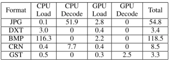
Format CPU Load
CPU Decode
GPU Load
GPU
Decode Total
JPG 0.1 51.9 2.8 0 54.8
DXT 3.0 0 0.4 0 3.4
BMP 116.3 0 2.2 0 118.5
CRN 0.4 7.7 0.4 0 8.5
GST 0.5 0 0.3 2.5 3.3
Table 1:Comparison of various timings in milliseconds for differ-ent compression schemes. We test our method against various for-mats rendering a set of frames from a360◦video at 4K resolution (3584×1792) similar to motion JPEG video [1992].
For fair comparison, we have chosen the maximum quality set-tings for Crunch and have chosen setset-tings for our method to be
E = 30, as described in Section 3.1. For these settings, on a typ-ical512×512texture, our method takes about0.76s to compress compared to the6.32s for Crunch. However, as can be seen in Fig-ure 7, our compression method has slightly larger variability than Crunch in terms of optimizing for rate-distortion. One of the main sources of this variability is the discrepancy in compressed index data, which is the least amenable to entropy encoding due to its incoherency (Figure 2). The only parameter that we can use to control the rate-distortion properties is the error thresholdE that is fairly coarse grained, as shown in Figure 6. The global dictio-nary of Crunch also gives it an advantage on hard-to-compress im-ages since neighboring redundancies are generally hard to find. To our benefit, however, using a truncated dictionary does improve the compression size for many textures in the Kodak data set, as shown in Figure 8. We present a breakdown of the size of each of the parts of a GST texture in Figure 10. This benefit arises due to the assumption that neighboring blocks produce similar palette indices during compression and as a result our method is dependent on the details of the image, similar to JPEG.
We use two main benchmarks for testing the performance benefits of our implementation. The first benchmark measures the average load time for all 600 4K resolution frames in a360◦video using a motion JPEG application similar to Pohl et al. [2014]. The sec-ond benchmark measures the time required to load all 128 Pixar textures, each with dimensions512×512, into GPU memory on a single CPU thread [Pixar 2015]. One of the main benefits of our method is the reduction in load times. We observe this benefit in both the batch load times for the Pixar dataset described in Table 2 and our360◦video benchmark in Figure 1. All results are mea-sured on desktop PC running Windows 7 on an Intel Xeon 8 core CPU and AMD R9 Fury GPU. As demonstrated in these results, the raw DXT1 load times are significantly faster than the super-compressed textures. Disk seek times and actual disk reads provide a significant amount of inconsistency in disk load timings. In our measurements we make sure that each of the files are fully loaded in the operating system’s page cache prior to doing any measurements in order to improve consistency. We observed significantly longer load times of high resolution DXT and BMP frames due to the full saturation of this cache. Our method, on the other hand, is partic-ularly well-suited to high resolution textures due to the increased parallelism offered in the GPU decoder.
Number of encoded symbols per thread
File size Local Table No Local Table
16 32 64 98 128 196 256 392 784 1568 1
1.2 1.4 1.6 1.8
2 2.5 3 3.5 4
Size (M
B)
T
im
e (m
s)
Figure 5:The affect of varying the number of symbols per decod-ing thread, and hence number of parallel decoders, as a compar-ison between average file size and decoding time of 600 frames of a 4K360◦video. When decoding few symbols per thread, size is dominated by storing many encoder states, although the increased parallelism helps decoding speed. Copying the ANS decoding table (Section 4) into local memory only benefits decoding speed when there is enough work per thread to benefit from fewer global reads.
Threshold vs. PSNR
0 20 40 60 80 100
28 31.5 35 38.5
42 Threshold vs. Size(KB)
0 20 40 60 80 1000
20 40 60 80 100
Kodak09
Kodak08 Kodak13
Kodak06
Figure 6:The difference in PSNR and compression size as a func-tion of our error threshold for a few images from the Kodak test suite. As we increase our error threshold, we see a decrease in the size of our index data and a drop in our PSNR. Both of these met-rics are sensitive based on the features of the encoded image. The PSNR stabilization after an increase in the error threshold supports the assumption of block-level coherency between indices.
7
Discussion
Based on the results in Section 6, we observe significant benefits from using a GPU-based decoding algorithm in the general case. In particular, very large textures are the most susceptible to the se-rial decoding requirements of traditional entropy encoders. In other applications, a multicore machine may parallelize the decoding of multiple low-resolution textures, which may be beneficial in terms of reducing the overhead of interfacing with the GPU. We observed that a set of per-core Crunch decoders processed all 128 textures of the Pixar dataset at similar load times to our method.
Limitations: Although our method presents many advantages, there are a few limitations in practice. First, our current imple-mentation requires additional scratch memory for intermediate re-sults during decompression. Although the additional memory is minimal, about 3X the size of the final texture, it may be a limit-ing factor for streamlimit-ing texture applications that try to exhaust the available GPU resources. However, this limitation may be over-come by using the final compressed texture as scratch memory, but this reduces efficiency by requiring unaligned memory reads and
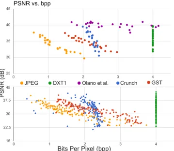
PSNR vs. bpp
Bits Per Pixel (bpp)
PSNR
(dB)
0 1 2 3 4
15 22.5 30 37.5 45
0 1 2 3 4
25 30 35 40 45
Crunch
Crunch GST JPG
JPEG DXT1DXT1 Olano et al.Olano et al.
Figure 7: We show PSNR versus bitrate values for our method against other compression schemes. The data shows that our method provides bit rates and quality comparable to the state of the art supercompressed textures. Each data point is an image in the (top) Kodak [1999] and (bottom) Pixar [2015] datasets with dimensions512×512.
Format JPEG PNG DXT1 Crunch GST
Time (ms) 848.6 1190.2 85.8 242.3 93.4 Disk size (MB) 6.46 58.7 16.8 8.50 8.91 CPU size (MB) 100 100 16.8 16.8 8.91
Table 2:Quantitative results of single-threaded loading of the 128 textures in the Pixar dataset [2015]. The CPU size represents the size of all textures in memory after any decoding procedure and prior to uploading to the GPU. The disk bandwidth is sufficiently fast to make decoding textures the bottleneck.
writes along with additional synchronization requirements. This sort of ’in-place’ decoding presents additional performance con-cerns by retrieving the values for individual channels in each of the endpoints as described in Section 5.
Additionally, the results in Section 6 are presented using our refer-ence implementation written in OpenCL for portability. However, during our experiments, we noticed significant stalls on the GPU that were unaccounted for. Our implementation would benefit from additional fine-grained control over the GPU programming inter-face, such as those presented in the Vulkan API, and further opti-mization could go a long way to realizing additional performance gains in our application.
Future Work: Although our implementation focuses on PVRTC and DXT1, more recent endpoint methods such as BPTC and ASTC have introduced increased complexity in the compressed represen-tation of textures [OpenGL 2010; Nystad et al. 2012]. They allow multiple palettes per block and variable bit depths for their palette indices. Additionally, ASTC provides variable index block dimen-sions that presents increased complexity to our re-encoding scheme. Although our method works with simple endpoint compressed for-mats, extensions to more complicated formats that preserve the ad-ditional quality may be possible.
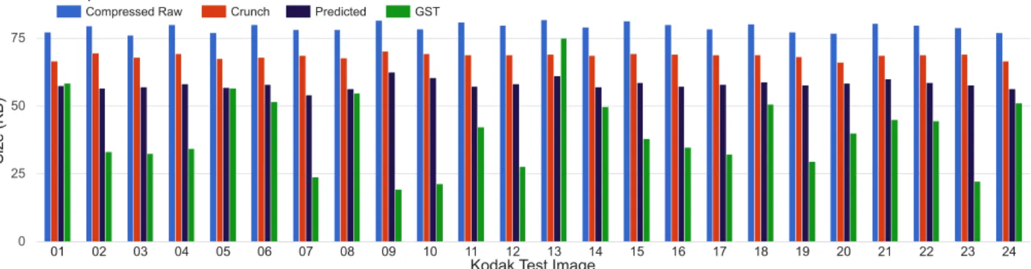
Compressed Indices Size
Compressed Raw Crunch Predicted GST
01 02 03 04 05 06 07 08 09 10 11 12 13 14 15 16 17 18 19 20 21 22 23 24
0 25 50 75
Kodak Test Image
Size (K
B)
Figure 8:We demonstrate a comparison of the compressibility of various approaches to preprocessing index data. This graph demonstrates the size of the compressed index data for various algorithms against the Kodak data set [1999] using the same Huffman encoder used in the Crunch textures. Palette indices are classically the most incoherent data in compressed textures. We show that by limiting the dictionary lookup to thekmost recently added dictionary entries, we increase the entropy encoding capabilities of the index data significantly over Crunch at maximum quality settings. Compressed raw is Huffman encoding applied to the unprocessed index data while the predicted method is the same method used by Str¨om and Wennersten [2011] applied to DXT textures.
Kodak23
DXT1 bpp:4.00
Crunch bpp:2.20 GST bpp:1.67 Original
Figure 9: A zoomed-in view of the visual quality of various com-pressed formats. The only stage in our compression pipeline that may introduce additional error is the re-encoding stage. Here we show that the amount of error introduced is imperceptible with re-spect to other DXT compression formats.
Size Breakdown vs. Error Threshold
CoCg Planes Y Plane Index Deltas Palette Dictionary
0 10 20 30 40 50 60 70 80 90 100
0 25 50 75 100
Error Threshold
Percent of
Total S
ize
Figure 10:An average of the percentage-wise breakdown of each of the constituent parts of a GST encoded texture using various er-ror thresholds. As we allow more erer-ror, the size of the dictionary decreases as a percentage of overall space consumed. We used both the Pixar and the Kodak data sets.
work. We also believe that the tabled compression formats such as ETC1 and ETC2 can be tackled using a variation of our algorithm. We do not expect our algorithm to emit compression rates as low as those presented by Str¨om and Wennersten [2011]. However, in-terpreting the parameters of tabled compressed textures as separate low-resolution images may significantly reduce the overhead of this class of compressed textures.
Although our benchmark uses360◦ video, our method is inher-ently designed for single-texture representations. A method similar to Olano et al [2011] is possible where an entire mip-map chain can be used to encode each of the individual endpoint images rather than an explicit wavelet transform. Additionally, the endpoint im-ages need not be compressed independently, as they have a lot of coherence that can be exploited to see additional gains in compres-sion performance.
Conclusions:We have presented a new algorithm for storing com-pressed textures on disk. The benefits of our algorithm show a sig-nificant improvement in decoding speed over state of the art CPU techniques. Furthermore, our algorithm provides a way to upload texture data directly to the GPU for decoding in order to maintain the CPU-GPU benefits. In particular, we believe that our method is best suited for streaming high-resolution textures from disk and net-work. In certain image-heavy applications, such as Google Street View, that require fast access to remote image data, and then ma-nipulate it using the GPU, we believe our method will provide the most benefit. Additionally, as more web page renderers move to the GPU, we believe that the improved decoding speed will be a boon for quickly introducing image data to mobile devices where decoding speed and responsiveness become increasingly important. As GPUs become more widespread in general, effective streaming solutions present a growing need.
8
Acknowledgements
This research is supported in part by ARO Contract W911NF-14-1-0437 and Google.
References
BEERS, A. C., AGRAWALA, M.,ANDCHADDHA, N. 1996. Ren-dering from compressed textures. InProceedings of the 23rd annual conference on Computer graphics and interactive tech-niques, ACM, SIGGRAPH ’96, 373–378.
BROWN, S., 2006. libsquish. http://code.google.com/p/libsquish/. BUCCIGROSSI, R. W., ANDSIMONCELLI, E. P. 1999. Image
compression via joint statistical characterization in the wavelet domain. IEEE Transactions on Image Processing 8, 12 (Dec), 1688–1701.
CASTANO˜ , I. 2007. High Quality DXT Compression using CUDA. NVIDIA Developer Network.
COHEN, A., DAUBECHIES, I., AND FEAUVEAU, J.-C. 1992. Biorthogonal bases of compactly supported wavelets. Commu-nications on Pure and Applied Mathematics 45, 5, 485–560.
DELP, E.,ANDMITCHELL, O. 1979. Image compression using block truncation coding. Communications, IEEE Transactions on 27, 9 (sep), 1335–1342.
DUDA, J. 2013. Asymmetric numeral systems as close to capacity low state entropy coders.CoRR abs/1311.2540.
FENNEY, S. 2003. Texture compression using low-frequency signal modulation. In Proceedings of the ACM SIG-GRAPH/EUROGRAPHICS conference on Graphics hardware, Eurographics Association, HWWS ’03, 84–91.
GELDREICH, R., 2012. Crunch. http://code.google.com/p/crunch/. GIESEN, F. 2014. Interleaved entropy coders. CoRR
abs/1402.3392.
HUFFMAN, D. A. 1952. A method for the construction of minimum-redundancy codes. Proceedings of the IRE 40, 9 (Sept), 1098–1101.
INADA, T.,ANDMCCOOL, M. D. 2006. Compressed lossless tex-ture representation and caching. InProceedings of the 21st ACM SIGGRAPH/EUROGRAPHICS Symposium on Graphics Hard-ware, GH ’06, 111–120.
IOURCHA, K. I., NAYAK, K. S.,ANDHONG, Z., 1999. System and method for fixed-rate block-based image compression with inferred pixel values. U. S. Patent 5956431.
KNITTEL, G., SCHILLING, A., KUGLER, A.,ANDSTRAßER, W. 1996. Hardware for superior texture performance.Computers & Graphics 20, 4, 475–481.
KODAK, 1999. Kodak lossless true color image suite. available at http://r0k.us/graphics/kodak.
KRAJCEVSKI, P., LAKE, A.,ANDMANOCHA, D. 2013. FasTC: accelerated fixed-rate texture encoding. InProceedings of the ACM SIGGRAPH Symposium on Interactive 3D Graphics and Games, ACM, I3D ’13, 137–144.
KRAJCEVSKI, P., GOLAS, A., RAMANI, K., SHEBANOW, M.,
ANDMANOCHA, D. 2016. VBTC: GPU-friendly variable block size texture encoding. Computer Graphics Forum 35, 2, 409– 418.
LESKELA, J., NIKULA, J.,ANDSALMELA, M. 2009. Opencl em-bedded profile prototype in mobile device. In2009 IEEE Work-shop on Signal Processing Systems, 279–284.
MALVAR, H. S., SULLIVAN, G. J.,ANDSRINIVASAN, S. 2008. Lifting-based reversible color transformations for image com-pression. InSPIE Applications of Digital Image Processing, In-ternational Society for Optical Engineering.
NYSTAD, J., LASSEN, A., POMIANOWSKI, A., ELLIS, S.,AND
OLSON, T. 2012. Adaptive scalable texture compression. In Proceedings of the ACM SIGGRAPH/EUROGRAPHICS confer-ence on High Performance Graphics, Eurographics Association, HPG ’12, 105–114.
OLANO, M., BAKER, D., GRIFFIN, W.,ANDBARCZAK, J. 2011. Variable bit rate GPU texture decompression. InProceedings of the Twenty-second Eurographics Conference on Rendering, Eu-rographics Association, Aire-la-Ville, Switzerland, Switzerland, EGSR ’11, 1299–1308.
OPENGL, A. R. B., 2010. ARB texture compression bptc. http:// www.opengl.org/registry/specs/ARB/texture compression bptc. txt.
PIXAR, 2015. Pixar one twenty eight. https: //community.renderman.pixar.com/article/114/
library-pixar-one-twenty-eight.html.
POHL, D., NICKELS, S., NALLA, R.,ANDGRAU, O. 2014. High quality, low latency in-home streaming of multimedia applica-tions for mobile devices. InComputer Science and Information Systems (FedCSIS), 2014 Federated Conference on, 687–694.
RISSANEN, J.,ANDLANGDON, G. G. 1979. Arithmetic coding. IBM J. Res. Dev. 23, 2 (Mar.), 149–162.
SHANNON, C. E. 1948. A mathematical theory of communication. The Bell System Technical Journal 27(July, October), 379–423, 623–656.
SKODRAS, A., CHRISTOPOULOS, C.,ANDEBRAHIMI, T. 2001. The JPEG 2000 still image compression standard. IEEE Signal Processing Magazine 18, 5 (Sep), 36–58.
STROM¨ , J.,ANDAKENINE-M ¨OLLER, T. 2004. PACKMAN: tex-ture compression for mobile phones. InACM SIGGRAPH 2004 Sketches, ACM, SIGGRAPH ’04, 66–.
STROM¨ , J., AND AKENINE-M ¨OLLER, T. 2005. iPACK-MAN: high-quality, low-complexity texture compression for mobile phones. In Proceedings of the ACM SIG-GRAPH/EUROGRAPHICS conference on Graphics hardware, ACM, HWWS ’05, 63–70.
STROM¨ , J., ANDPETTERSSON, M. 2007. ETC2: texture com-pression using invalid combinations. InProceedings of the 22nd ACM SIGGRAPH/EUROGRAPHICS symposium on Graphics hardware, Eurographics Association, GH ’07, 49–54.
STROM¨ , J., AND WENNERSTEN, P. 2011. Lossless compres-sion of already compressed textures. InProceedings of the ACM SIGGRAPH Symposium on High Performance Graphics, ACM, HPG ’11, 177–182.
TORBORG, J.,ANDKAJIYA, J. T. 1996. Talisman: Commodity re-altime 3d graphics for the PC. InProceedings of the 23rd Annual Conference on Computer Graphics and Interactive Techniques, ACM, New York, NY, USA, SIGGRAPH ’96, 353–363. WALLACE, G. K. 1992. The JPEG still picture compression
stan-dard. IEEE Transactions on Consumer Electronics 38, 1 (Feb), xviii–xxxiv.