EFFICIENT LIGHT AND SOUND PROPAGATION IN REFRACTIVE MEDIA
WITH ANALYTIC RAY CURVE TRACER
Qi Mo
A dissertation submitted to the faculty of the University of North Carolina at Chapel Hill in partial fulfillment of the requirements for the degree of Doctor of Philosophy in the Department of Computer
Science.
Chapel Hill 2015
c O2015
Qi Mo
ABSTRACT
QI MO: EFFICIENT LIGHT AND SOUND PROPAGATION IN REFRACTIVE MEDIA WITH ANALYTIC RAY CURVE TRACER. (Under the direction of Dinesh Manocha.)
Refractive media is ubiquitous in the natural world, and light and sound propagation in refractive me-dia leads to characteristic visual and acoustic phenomena. Those phenomena are critical for engineering applications to simulate with high accuracy requirements, and they can add to the perceived realism and sense of immersion for training and entertainment applications. Existing methods can be roughly divided into two categories with regard to their handling of propagation in refractive media; first category of meth-ods makes simplifying assumption about the media or entirely excludes the consideration of refraction in order to achieve efficient propagation, while the second category of methods accommodates refraction but remains computationally expensive. In this dissertation, we present algorithms that achieve efficient and scalable propagation simulation of light and sound in refractive media, handling fully general media and scene configurations.
Our approaches are based on ray tracing, which traditionally assumes homogeneous media and rectilinear rays. We replace the rectilinear rays with analytic ray curves as tracing primitives, which represent closed-form trajectory solutions based on assumptions of a locally constant media gradient. For general media profiles, the media can be spatially decomposed into explicit or implicit cells, within which the media gradient can be assumed constant, leading to an analytic ray path within that cell. Ray traversal of the media can therefore proceed in segments of ray curves.
The first source of speedup comes from the fact that for smooth media, a locally constant media gradient assumption tends to stay valid for a larger area than the assumption of a locally constant media property. The second source of speedup is the constant-cost intersection computation of the analytic ray curves with planar surfaces. The third source of speedup comes from making the size of each cell and therefore each ray curve segment adaptive to the magnitude of media gradient. Interactions with boundary surfaces in the scene can be efficiently handled within this framework in two alternative approaches. For static scenes, boundary surfaces can be embedded into the explicit mesh of tetrahedral cells, and the mesh can be traversed and the embedded surfaces intersected with by the analytic ray curve in a unified manner. For dynamic scenes,
implicit cells are used for media traversal, and boundary surface intersections can be handled separately by constructing hierarchical acceleration structures adapted from rectilinear ray tracer. The efficient handling of boundary surfaces is the fourth source of speedup of our propagation path computation. We demonstrate over two orders-of-magnitude performance improvement of our analytic ray tracing algorithms over prior methods for refractive light and sound propagation.
To my family,
my parents Lifeng Mo and Youhong Tao, and my husband Fei Zhao.
ACKNOWLEDGMENTS
Writing a doctorate thesis is never an easy endeavor. I would venture to say that mine has been especially hard, with a cancer diagnosis right after my preliminary exam. The timing was most unfortunate, as after a year and a half of treatment the research topic and ideas that I had all became obsolete. I am able to finish this work presented here, solely because of the people that I am about to mention. I am forever indebted to them.
First of all, I would like to thank my advisor, Prof. Dinesh Manocha, for his constant guidance and support, and for saying to me ”Sometimes research is all about perseverance”, which I needed to hear. I would also like to thank the members of my committee, Prof. Gary Bishop, Prof. Ming C. Lin, Prof. Anselmo Lastra, and Prof. Marc Niethammer, for their invaluable feedback and support.
I have learned a tremendous amount from my many talented collaborators, including Christian Lauter-bach, Micah Taylor, Anish Chandak, and Hengchin Yeh. I am equally grateful to have the privilege of knowing all my co-works in GAMMA group, many of whom have become friends over the years. Thanks are also due to the excellent staff at the Department of Computer Science at UNC-Chapel Hill, and I would like to thank Jodie Turnbull, Janet Jones, and Tim Quiggs in particular, for rooting for me and accommodating the numerous unconventional arrangements that I had to make due to my illness. A special shout-out goes to Dr. Carey Anders, Dr. Keith Amos, Dr. Ellen Jones, my medical team at UNC Health Care, and at Get REAL & HEEL, for bringing me back to life, literally and metaphorically.
TABLE OF CONTENTS
LIST OF TABLES . . . xi
LIST OF FIGURES . . . xiv
1 Introduction . . . 1
1.1 Refractive Propagation and Its Applications . . . 1
1.1.1 Refractive Media for Light Propagation . . . 2
1.1.2 Visual Applications . . . 4
1.1.3 Refractive Media for Sound Propagation . . . 7
1.1.4 Acoustic Applications . . . 9
1.2 Propagation Simulation . . . 12
1.2.1 The Rendering Pipeline . . . 12
1.2.2 The Propagation Stage . . . 14
1.2.3 Similarity Between Light and Sound Propagation . . . 16
1.2.4 Differences Between Light and Sound Propagation . . . 17
1.3 Challenges . . . 18
1.4 Thesis Statement . . . 18
1.5 Contributions . . . 19
1.5.1 Explicit cell method with analytic ray curve tracing . . . 19
1.5.2 Implicit cell method with dynamic ray curve tracing . . . 20
1.5.3 Acoustic field computation with ray curve tracing and
Gaussian beam . . . 20
1.6 Thesis Outline . . . 21
2 Background . . . 23
2.1 Physics of propagation in refractive media . . . 23
2.1.1 Refractive media properties . . . 23
2.1.2 Common media profiles . . . 24
2.2 Simulation of Light Propagation . . . 27
2.2.1 The Rendering Equation . . . 27
2.2.2 Rectilinear Ray Tracing . . . 29
2.2.3 Piece-wise Rectilinear Ray Tracing . . . 30
2.2.4 Curved Ray Tracing . . . 31
2.3 Simulation of Sound Propagation . . . 31
2.3.1 The Acoustic Wave Equation and Wave-based Methods . . . 31
2.3.2 Geometric Acoustics and Rectilinear Ray Tracing . . . 33
2.3.3 Piecewise Rectilinear Ray Tracing . . . 34
2.3.4 Curved Ray Tracing . . . 35
2.4 Appendices . . . 35
2.4.1 Derivation of analytic ray curves . . . 35
2.4.2 Other known analytic ray solutions . . . 37
3 Explicit Cell Method with Analytic Ray Curve Tracing . . . 40
3.1 Overview . . . 40
3.2 Algorithm . . . 41
3.2.2 Adaptive Mesh . . . 43
3.2.3 Embed Media Boundaries . . . 43
3.2.4 Surface Interactions . . . 44
3.3 Implementation . . . 44
3.3.1 Construction of Adaptive Mesh . . . 44
3.3.2 Embedding of Boundary Surfaces . . . 45
3.3.3 Gradient estimation . . . 46
3.4 Results and Analysis . . . 47
3.4.1 Benchmarks . . . 47
3.4.2 Error analysis of adaptive mesh . . . 48
3.4.3 Error analysis of ray curve tracer . . . 49
3.4.4 Comparison to numerical ray integration . . . 51
3.4.5 Comparison to prior analytic ray curve . . . 54
3.4.6 Performance of ray curve tracer . . . 56
3.4.7 Applications on outdoor acoustics . . . 58
3.5 Discussions . . . 59
3.6 Appendices . . . 61
3.6.1 Considerations of embedded mesh . . . 61
3.6.2 Gradient estimation solutions . . . 61
3.6.3 Comparison of meshes generated from local gradients ofn, c, n2 . . . . 64
4 Implicit Cell Method with Dynamic Ray Curve Tracing . . . 67
4.1 Overview . . . 67
4.2 Algorithm . . . 68
4.2.1 Analytic Ray Curve . . . 68
4.2.2 Ray Tracing Algorithm . . . 70
4.3 Results . . . 74
4.3.1 Performance Comparison of Ray Models . . . 74
4.3.2 Outdoor Applications of Analytic Ray Tracer . . . 78
4.4 Discussions . . . 80
5 Acoustic Field Computation with Ray Curve Tracing and Gaussian Beam. . . 83
5.1 Overview . . . 83
5.2 Algorithm . . . 84
5.2.1 Analytic Dynamic Ray Tracing . . . 84
5.2.2 Gaussian Beam Field Computation . . . 86
5.3 Implementation . . . 87
5.4 Results . . . 90
5.4.1 Validation . . . 90
5.4.2 Applications on Complex Outdoor Sound Field . . . 94
5.5 Discussions . . . 96
6 Conclusion . . . 97
6.1 Explicit Cell Method with Analytic Ray Curve Tracing . . . 97
6.2 Implicit Cell Method with Dynamic Ray Curve Tracing . . . 98
6.3 Acoustic Field Computation with Ray Curve Tracing and Gaus-sian Beam . . . 98
6.4 Future Work . . . 99
LIST OF FIGURES
1.1 Inferior and superior mirages in a refractive atmosphere. . . 2
1.2 Other visual phenomena of a refractive atmosphere. . . 3
1.3 Refractive media in movies: applications of light propagation simulation. . . 5
1.4 Refractive media in virtual reality for training applications. . . 6
1.5 Engineering applications of propagation simulation of light and sound: Lidar and Sonar. . . 6
1.6 Standard model of sound speed profiles in the atmosphere and the ocean and the corresponding propagation trajectories. . . 10
3.1 Analytic ray curves: known solutions of propagation trajectories for certain media profiles. . . 42
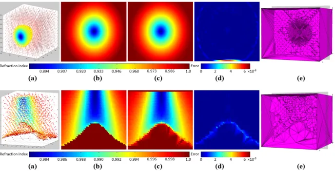
3.2 Adaptive tetrahedral meshes representing media profiles. . . 42
3.3 Error analysis of the adaptive meshes approximating the under-lying media profiles. . . 48
3.4 Compare to error analysis of the octree approximating the under-lying media profiles. . . 49
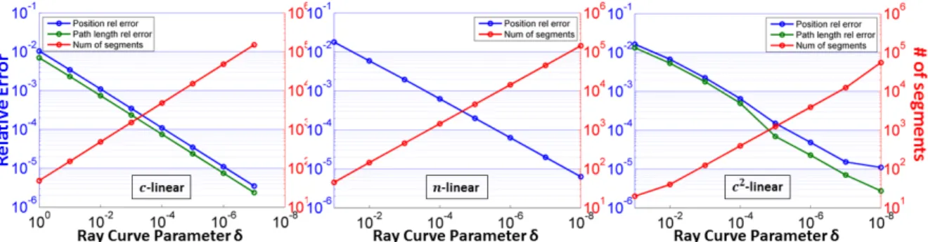
3.5 Convergence of the ray curve tracer on media profiles with ana-lytic ground truth in terms of the positions on propagation paths and the path lengths. . . 50
3.6 Comparison of convergence between the analytic ray curve tracer and both higher-order and adaptive numerical ray integration: mirage media profiles. . . 50
3.7 Comparison of convergence between the analytic ray curve tracer and both higher-order and adaptive numerical ray integration: logarithmic sound speed profiles. . . 50
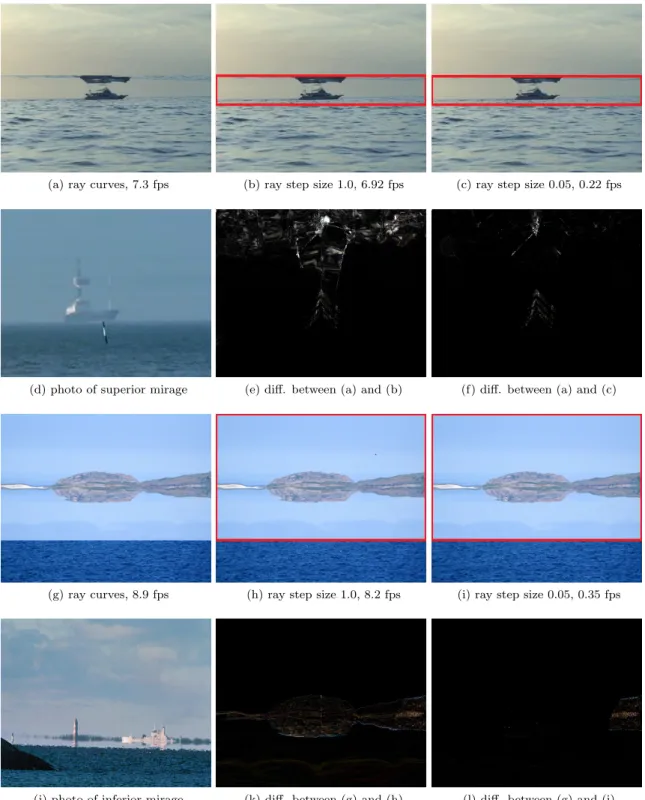
3.8 Same-quality/same-speed comparisons between analytic ray curve tracer and numerical ray integration: visual rendering of mirages. . . 52
3.9 Adaptive meshes built for the elephant benchmark at two different resolutions by a control parameter. . . 53
3.10 Convergence of ray curve tracer results on the elephant bench-mark: measured in the positions, tangent directions along the propagation paths and the path lengths. . . 53
3.11 Same-speed comparisons of different combinations of ray curve
primitives and ray tracing data structures: the elephant benchmark. . . 55
3.12 Performance of the ray curve tracer and scalability with the mag-nitude of media variations, media mesh complexity, and scene surface complexity. . . 57
3.13 Benchmark results of acoustic propagation in the atmosphere: up-ward and downup-ward refraction. . . 58
3.14 Acoustic propagation in the atmosphere: local temperature vari-ations and wind profiles. . . 59
3.15 Application of the analytic ray tracer on outdoor acoustic simulation. . . 60
3.16 Comparison between embedding and linking boundary surfaces. . . 62
3.17 Comparisons of meshes built for the 3 analytic ray curves: upward refractive atmosphere. . . 65
3.18 Comparisons of meshes built for the 3 analytic ray curves: down-ward refractive atmosphere. . . 66
4.1 Parabolic ray curves and overview of the ray curve tracing algorithm. . . 71
4.2 Efficient media traversal with the ray curve tracer. . . 72
4.3 Efficient surface intersection with the ray curve tracer. . . 73
4.4 Ray trajectories computed by the ray curve tracer for atmospheric and oceanic sound speed profiles. . . 76
4.5 Cost and accuracy trade-off comparison between the ray curve tracer and 4th order Runge-Kutta ray integration: scaling with the magnitude of media variations. . . 78
4.6 Adaptive segment sizes used by the ray curve tracer for ocean acoustic propagation. . . 79
4.7 The application of the dynamic ray curve tracer on outdoor benchmarks. . . 79
4.8 Visualization of the cost of ray-surface intersection: efficiency of hierarchical data structures for surface culling. . . 80
5.1 Sound field computation with analytic ray tracer and Gaussian
beam: algorithm overview. . . 84 5.2 Analytic ray curve and the analytic evolution of ray-centered coordinates. . . 85 5.3 Validation benchmark A Range-Transmission Loss (TL) plot:
dif-ferent atmospheric profiles. . . 91 5.4 Validation benchmark A 2D field: downward refractive atmosphere. . . 92 5.5 Validation benchmark B 2D field: Munk profile with conical seamount. . . 93 5.6 Acoustic pressure difference field difference for source in the
val-ley: upward vs. downward refraction. . . 94 5.7 Acoustic pressure difference fields for source on the slope: upward
vs. downward refraction, and upwind vs. down wind. . . 95 5.8 Acoustic pressure difference field between vector winds of opposite
directions for source in the valley. . . 95 5.9 Outdoor benchmark and acoustic pressure field results. . . 96
LIST OF TABLES
3.1 Benchmark outdoor scenes and the stats of the meshes constructed
for ray tracing. . . 47 3.2 Same-quality comparisons of different combinations of ray curve
primitives and ray tracing data structures: the elephant benchmark. . . 54 3.3 Breakdown of analytic ray curve traversal time. . . 57
4.1 Same-quality comparison between the ray curve tracer and 4th
order Runge-Kutta ray integration. . . 77 4.2 Same-speed comparison between the ray curve tracer and 4th
Chapter 1
Introduction
Refraction refers to the change of propagation direction of a sound or light wave because of a speed gradient; waves no longer follow straight-line paths under refraction. Refractive media is ubiquitous in the physical world. The atmosphere, even under stable conditions, has spatially varying temperature, pressure, and humidity (USGPC, 1976). There can be wind fields or other weather patterns that affect the underlying distribution of atmospheric properties (Monin and Obukhov, 1954; Businger et al., 1971; Panofsky and Dutton, 1984a). Similarly, the ocean displays spatially varying properties such as temperature, pressure, and salinity, and there are flow patterns like currents and eddies that modify those properties (Jensen et al., 2011). Such profiles of properties determine the propagation speed of sound or light waves at any particular spatial location and time within a medium.
Simulation of light and sound propagation is a critical component for visual and acoustic rendering (Ch. 1.2.1), and for refractive media it remains a challenging problem as the computational cost can become prohibitively expensive. Existing propagation methods either ignore refraction or make simplifying assump-tions about the problem domain to keep the computation tractable (Ch. 2.2 and 2.3), yet for a range of important applications such simplification is not acceptable (Ch. 1.1). This thesis presents algorithms that improve the efficiency of sound and light propagation in refractive media, and enable simulation of fully gen-eral three-dimensional media, complex and large scenes, and dynamic configurations at close to interactive performance.
1.1 Refractive Propagation and Its Applications
(a) (b) (c)
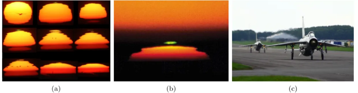
Figure 1.1: Mirages: (a)inferior mirage,(b)superior mirage,(c)Fata Morgana. (Explained in Ch. 1.1.1). Image sources: (a) (Gil, 2013) (b) (Parviainen, 2002) (c) (Cartier, 2008).
1.1.1 Refractive Media for Light Propagation
Continuous variation of light refractive indices (or equivalently, light propagation speed) exists in different media in the natural world, including the atmosphere and human soft tissues. Man-made artifacts such as gradient-index lenses use special manufacturing techniques to achieve the continuously varying profile of properties in order to manipulate the light propagation paths in their interior.
Atmosphere
The light index of refraction in the atmosphere depends on humidity and density of the air (Owens, 1967; Gladstone and Dale, 1858). While the effect of humidity on light propagation is usually very subtle (Ciddor, 1996), density, which is a function of pressure and temperature, can change light trajectories significantly (Siebren and van der Werf, 2003). The variation in refractive indices is greatest in the layers of atmosphere close to the ground, where pressure can be assumed to be constant (Ciddor, 1996). Therefore, temperature is the leading factor that determines the atmospheric refractive index. Common visual phenomena produced by light refraction in the atmosphere include mirages, distortion of horizons and celestial bodies, and localized distortion near heat sources (Minnaert and Seymour, 1993).
(a) (b) (c)
Figure 1.2: Visual phenomena of a refractive atmosphere: (a) distorted sun, (b) green flash, (c) heat shimmering. See detailed explanation for each of these phenomena in Ch. 1.1.1. Image sources: (a) (Inaglory, 2006) (b) (Young, 2012) (c) (Lucas, 2013).
inferior and superior mirages concatenating together (Fig. 1.1c).
During sunrise or sunset, the sun can appear to be flattened, split, or have a double image, depending on the layering of atmospheric profiles (Fig. 1.2a). Both the flattened and the double sun result from conditions similar to inferior mirages when the sun light is bent upward to different degrees. The split sun happens, on the other hand, when part of the light that travels closer to the ground is bent downward by refraction or total internal reflection while the remaining light stays undistorted. Furthermore, the refractive index profiles differ for different wavelengths, so the dispersion of sunlight can produce the phenomenon known as “green flash”, when green light rays are bent more downward which form a green halo on top of the image of the sun (Fig. 1.2b) (Young, 2000).
Besides the overall temperature profile, there are often localized heat sources and temperature fluctuations from fire, the jet of an airplane, a valley where the heat could be trapped, a sprawling city with its own micro-climate as a “heat island”. The resulting visual phenomena include various forms of heat haze and heat shimmering (Fig. 1.2c).
Human Tissues
Soft tissues in the human body are naturally heterogeneous and composed of various structures spanning several orders of magnitude in size and a wide range of materials (Jacques, 2013). The interconnection of human tissues often leads to the resulting density and refractive index being a continuous spatial distribution (Ding et al., 2006; Bashkatov et al., 2011). Research using phase-contrast microscopy has observed that the inhomogeneous refractive indices in tissues fit the classical model of atmospheric turbulence (Schmitt and Kumar, 1996). The light refractive properties of tissues are also affected by the underlying hydration, as well as other physiological or pathological conditions of human body, adding to the variation in the profiles.
Lenses
Physical processes such as advection and diffusion often lead to non-uniform distribution of material properties, and these processes are utilized in different manufacturing techniques to make objects with varying interior optical profiles. A good example is gradient-index (GRIN) lenses, which refer to lenses with a gradual variation of refractive index (Gomez-Reino et al., 2012; Bociort, 1994). GRIN lenses may have a gradient of the refractive index that is spherical, axial, or radial, corresponding to different applications.
For example, a radial profile of nearly parabolic shape leads to rays following sinusoidal trajectories throughout the length. The length of such a GRIN lens thus controls whether the light rays will come out of the lens focused or collimated or somewhere in-between. Such GRIN lenses are used as relay devices for endoscopy, in laser diode beam shaping, and for optical coherence tomography. In a GRIN lens with a radially varying profile, all optical paths (refractive index multiplies distance) are the same, which, when used to make optical fibers for telecommunications, reduces modal dispersion and allows for a higher temporal bandwidth than traditional models that rely on total internal reflection.
GRIN lenses have certain properties that are superior to traditional lenses. With GRIN lenses, the light rays’ trajectories are manipulated by the varying refractive index profile instead of the shape of the lens surfaces. GRIN lenses are therefore often manufactured to have flat surfaces, which avoid spherical aberrations of traditional lenses, simplifies the manufacturing and mounting process, and facilitates seamless coupling of different components to form an optical assembly. The planar geometry of a GRIN lens also makes designing and tuning of the optical characteristics much more cost-effective (Gomez-Reino et al., 2012; Bociort, 1994).
Human or other mammals’ eyes are the examples of gradient-index lenses occurring in nature (Deering, 2005; Ji et al., 2012). In human eyes the refractive index varies between 1.386 and 1.406, allowing the eye to image with good resolution and low aberration at a range of distances.
1.1.2 Visual Applications
(a) (b) (c)
Figure 1.3: Visual applications: movie-making. Phenomena from refractive light propagation lead to iconic imagery in movies (Ch. 1.1.2): (a)Desert scene inLawrence of Arabia. (b)Fire distorting everything in view fromGhost Rider, (c)Heat haze fromMad Max: Fury Road.
Entertainment and Training
Movies nowadays contain abundant visual effects that are either completely computer generated, or have a large number of frames with computer imagery and real footage composited together. The spectacles of refractive light propagation in the atmosphere (see Ch. 1.1.1) constitute iconic images for numerous movies (e.g. mirage scene in Lawrence of Arabia, Fig. 1.3a), and has even been used as plot device (The Green Flash). Fire is also an important element of scenes such as explosions that are often the visual focal point (Fig. 1.3b). Furthermore, computer generated images often need to have the capability of matching and blending in with real frames, so the capability of replicating physical reality is highly desirable. For games, the requirement of high visual fidelity is combined with the constraints of interactivity with tight computational and memory budgets, for which efficiency of simulation is of utmost importance.
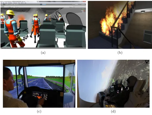
Virtual reality(VR) is used for training purposes for a variety of applications, especially for scenarios that are rare or difficult to manage in real settings. The level of realism achieved in VR training systems determines the immersion of the trainee and in turn the effectiveness of training. VR training applications that benefit particularly from high-fidelity simulation of light propagation include military training for desert environments (Pellerin, 2011), therapy and rehabilitation systems for post-traumatic stress disorder (Gerardi et al., 2008; Spelman et al., 2012), emergency evacuation training for fire or other hazards (Sharma and Jerripothula, 2015; Sharma et al., 2014; Wilkerson et al., 2008; Vincent et al., 2008; Ragan et al., 2010), flight simulators for atmospheric conditions (Nielsen, 2003; Daniels et al., 2012), and driving simulators with weather modules (Bella and Calvi, 2013; Bella and Calvi, 2013). Most existing systems have yet to incorporate refraction-related phenomena, mostly because of the lack of efficient algorithms that can achieve interactive performance.
(a) (b)
(c) (d)
Figure 1.4: Visual applications: training. Phenomena from refractive light propagation rendered in training VR systems (Ch. 1.1.2): (a) Subway evacuation and (b) fire evacuation. The realism of fire rendering could benefit from simulating light refraction. (c) Driving simulators: weather conditions that cause light refraction are important for safety tests. (d) Flight simulators: the rendering of aerial views including atmospheric refraction contributes to users’ sense of immersion. Image source: (a) (Sharma et al., 2014) (b) (Smith, 2015)) (c) (de Winter et al., 2007) (d) (Daniels et al., 2012).
(a) (b)
Engineering
For entertainment and training, the requirement for light propagation simulation is to produce physically realistic visual results for human observers. For engineering applications described in this section, on the other hand, accurate numerical results are desirable.
In the atmosphere, light propagation simulation is used in solar radiation modeling (Badescu, 2008; Pavlov and Pavlova, 2010; Hofierka et al., 2002; Muneer and Kambezidis, 1997; Robertson and Flury, 2014) to compute the absorption, transferring, and dispersion of solar energy, the result of which has important implications for agriculture, environmental protection, and public health. Laser ranging technology (e.g. Lidar (Guenther et al., 2000; Prezhdo et al., 2005)) is another application that relies on computing the path length and travel time of light propagating in the atmosphere, for which accounting for refractive light paths that are curved can be critical for the accuracy of the measured range (Yuan et al., 2011; Guenther et al., 2000; Prezhdo et al., 2005; Degnan, 1993; Dodson, 1986; Gardner, 1977).
Both diagnostic and therapeutic applications depend on modeling and simulating light propagation through tissues. For the former, light propagates in a tissue before emerging for detection; for the latter, light propagates in a tissue and deposits energy via absorption at locations determined by the underlying tissue properties. Moreover, there are novel medical imaging technologies that benefit from accurate simulation of light refraction in particular. Optical clearing (Rogers et al., 2013; Shen and Wang, 2011; Malektaji et al., 2014), for example, manipulates the tissue properties with mechanical compression so that a microscope can produce clear images of focal planes that are deep within thick tissue samples. Hybrid acoustic-optic technology such as ultrasound-modulated optical tomography (Powell and Leung, 2012) is another novel application that combines the optical contrast and the spatial resolution of ultrasound fields; the change in tissue refractive index by acoustic compression and rarefaction needs to be accurately modeled to achieve the desired precision.
For GRIN lenses, simulating the refractive propagation paths of light inside the lenses facilitates both the design and the manufacturing processes. As these applications strive to mimic the physical world as closely as possible, the scale and the complexity of the problems present great challenges for the simulation methods of light propagation.
1.1.3 Refractive Media for Sound Propagation
The propagation speed of sound varies throughout the two most prominent acoustic media in nature: the atmosphere and the ocean. In this section we introduce the atmospheric and ocean profiles from the sound propagation perspective, and the acoustic phenomena produced by the refraction of sound waves in these
media (Fig. 1.6).
Atmosphere
The atmosphere is a refractive medium for sound waves that leads to significant acoustic effects (Salomons, 2001a). Diurnal change of sound propagation is routinely observed (Hohenwarter and Mursch-Radlgruber, 2014; Wilson, 2003; Prospathopoulos and Voutsinas, 2007): during the day, when the temperature is typically higher closer to the ground, sound waves tend to refract upward, creating a shadow zone with very low level received sound (Figure 3.13a); when the temperature gradient is inverted at night, sound waves are refracted downward, intensifying the acoustic signals received by the listener. Downward refraction combined with a reflective ground or water surface creates a set of concentric circular patterns in the sound field around a source (Figure 3.13d).
Wind also plays a critical part in atmospheric sound propagation. The wind speed can be significant compared to the sound speed (Lamancusa and Daroux, 1993b), and the strength and directional distribution of the wind gives rise to intricate sound fields. In the simplest scenario, with a wind field of uniform direction and velocity, the sound level from a source will be stronger in the downwind direction than the upwind direction. The wind field also interacts with the temperature and pressure field, as can be simulated with a comprehensive background flow system (Zheng and Li, 2008).
The shape of terrains not only affects the course of sound propagation itself, but it also alters the temperature and wind profile above it, and thus influences sound paths additionally in an indirect way. A hill shapes the wind profile differently on its wind-facing side versus the back slopes, and the changes in wind profile can reach high above the hilltop (Lamancusa and Daroux, 1993a). A valley can create airflow in the longitudinal direction, as well as upward airflow on the slopes (Heimann and Gross, 1999; Renterghem et al., 2007a; Heimann et al., 2010; Heimann, 2006; B´erengier et al., 2003). Material properties of different types of land covers matter as well, e.g. grassland or trees (Heimann, 2003) can modify the atmospheric profile much differently from hard ground.
Ocean
The ocean constitutes another vast refractive media for sound propagation (Urick, 1983). The oceanic sound speed profile has a strong dependency on depth, but it also has complex 3D variations based on the temperature, salinity, pressure distributions (Medwin, 1975). Similar to the role of wind for atmospheric acoustics, the ocean currents play a significant part in guiding the sound wave propagation. The bottom bathymetry and its impedance can be just as complicated and of comparable scale with terrains on land. Particles such as salt, debris, air bubbles, droplets, as well as larger dynamic structures such as eddies are important sound scatterers (Colosi, 2006; Jian et al., 2009). The water surface, when it is stable and smooth, forms an almost perfect reflector of sound; when it is rough with waves, the surface can act as a scatterer as well (Siderius and Porter, 2008).
Ocean acoustics often differentiates between deep sea propagation, for which the focus is on long-range channels (Virovlyansky, 2003) arising from refractive propagation guided by the media profile (Fig. 1.6d), and the shallow coastal regions (often defined by water depth less than 200m). In shallow water, the temporal and spatial variations of sound speed profiles are more significant with natural variability of the temperature of shallow water, seasonal wind cycles and frequently passing weather fronts, the strong salinity gradients from river outflows. The variable surface conditions lead to intricate scattering, unlike the mostly specular reflection from calm water. In addition, sound interactions with the sea bed (Ballard et al., 2012; Ballard, 2012) requires an understanding of the sedimentary structure and shape of the bottom to a level of detail that is usually not required in deep water.
In shallow regions as well as in deep sea, sound from human activity drives the changes in the ocean soundscape. Active sonar systems, seismic-exploration activity, maritime shipping, offshore and coastal wind farms all disrupt the natural acoustic environment and result in noise pollution that needs to be monitored and regulated. Furthermore, animals can generate or scatter sound. Ocean mammals including whales and dolphins rely on sound production and reception to navigate, communicate, and hunt, with their innate understanding of sound propagation in the ocean.
1.1.4 Acoustic Applications
Similar to light, applications of sound propagation simulation can be categorized into those for generating sound for human listeners, and those for computing numerical results like acoustic pressure amplitudes and propagated signals for engineering purposes.
(a) (b)
(c) (d)
Figure 1.6: Standard model of sound speed profiles in the atmosphere and the ocean. (a,c)The US Standard Atmosphere (USGPC, 1976) profile of temperature, density, pressure, and the resulting sound speed with altitude; and the Munk profile for the ocean, respectively. (b,d)Example ray plots that illustrate the impact of refractive media under a downward refractive atmosphere, and the Munk profile, respectively.
Training and entertainment
outdoor propagation effect is essential.
For entertainment purposes, sound rendering is also gaining attention in both movie and game industries. The trend is moving towards physical simulation of sound propagation and away from pre-recording and Foley artistry (Raghuvanshi, 2010; Antani, 2013). There exists an abundance of outdoor scenes in movies and games that will benefit from realistic acoustic propagation phenomena.
Engineering
Engineering applications of sound propagation simulation include urban planning, noise control, and underwater exploration and communication, marine biology, as well as shipping and other industrial planning. For these applications, the accuracy requirement is high and ignoring the propagation effect caused by refractive media leads to unsatisfactory results. On the other hand, the simulation computation needs to be efficient and practical to handle the real-world complexity of the problem domain.
In the atmosphere, noise control requires consideration of a complicated combination of the meteorological conditions and intervening terrain and man-made structures. Many empirical and semi-empirical schemes (Attenborough et al., 2006a) have been proposed to predict the noise level for particular types of sound sources (road traffic, rail traffic, industry, or aircraft) and for categorized terrains, land covers, and meteorology. Efforts have also been made towards a comprehensive noise prediction model that covers all the specific predictors (Defrance et al., 2007). However, such empirical models fail to provide highly-accurate, fine-grained predictions for individual scenarios. Given the availability of detailed terrain and meteorology data, running a fully general sound propagation simulation would be ideal if not for the computational cost (Oshima et al., 2013a).
In the ocean, noise control is equally important for protecting marine ecosystems (Nosengo et al., 2009) and for preventing acoustic pollution sources such as sonar clutters from disrupting human activities (Zam-polli et al., 2013; McDonald et al., 2006; McDonald et al., 2008; Nedwell and Howell, 2004). In addition, sound propagation is utilized for ocean assessment (Hoffman et al., 2001), navigation (Aparicio et al., 2011), as well as underwater communication and data transfer (Fig. 1.5b). Many frequencies such as ultraviolet rays and radio signals do not propagate well in water. Sound waves, on the other hand, propagate well over long distances underwater. As a result, specialized telephone systems have been built to transmit and receive human vocal sound waves through hydrophones and audio amplifiers, and digital data such as words and images can be transferred via acoustic modems which convert them into underwater sound signals (University of Rhode Island, 2015). Such underwater acoustic networks (Wang et al., 2013a; PhysOrg.com, 2009; Akyildiz et al., 2004; Akyildiz et al., 2005; Chandrasekhar et al., 2006) are necessary for applications
like submarine maneuvering, and remote acquisition of oceanographic research data. It is also an enabling technology for the operation of unmanned underwater vehicles (Wang et al., 2010), which are utilized by a wide range of military, industrial, and scientific applications.
1.2 Propagation Simulation
Light and sound are both wave phenomena, and they constitute the visual and auditory sensory input, respectively, that are most important for human perception. Light is an electromagnetic wave, while sound is a mechanical wave. Light and sound are governed by different forms of wave equations, and simulating their propagation and the corresponding phenomena has wide and important applications (those most pertaining to this work are listed in Ch. 1.1.2 and 1.1.4).
In this section we first introduce the common way of organizing propagation simulation: the rendering pipeline (Ch. 1.2.1), and then we focus on the propagation stage of the rendering pipeline and the range of possible interactions between the waves and surfaces or media within that stage (Ch. 1.2.2). We present light and sound propagation side by side to highlight their similarities (Ch. 1.2.3), which are the basis for many shared simulation methodology between them. On the other hand, each has its unique challenges, and Ch. 1.2.4 covers the differences and comparisons between light and sound propagation simulation.
1.2.1 The Rendering Pipeline
The propagation simulation takes light or sound sources and the scenes in which the light or sound waves travel as input, and the aim is to compute the light or sound received by the receivers. Both light and sound simulation are often organized into a rendering pipeline with three stages: source modeling, propagation, and receiver computation. The propagation stage connects sources with receivers and simulates how light or sound wave spread through space. It is often the most computationally-intensive stage of the pipeline, and is the focus of this thesis.
Source Modeling
For sound sources, the position and directivity are also important characteristics. Additionally, signals emitted by sound sources are usually modeled as time-dependent (unlike light sources, see Ch. 1.2.4 for details). The source signal can either be pre-recorded, orsynthesized from directly modeling the vibrations of sounding objects (Cook, 2002). Two of the simplest idealized sound sources are a harmonic point source and a source emitting harmonic plane waves. More complex sources are usually decomposed into harmonic waves before propagating. For time-domain simulation, propagation produces an impulse response as the result, which is then convolved with the source signal.
Propagation
Propagation models the spreading of light and sound waves from the source, and it encompasses various interactions with the scene. A common way of looking at a propagation simulation involves two aspects: finding propagation paths that connect the source and the receiver, and computing the physical quantities (energy, intensity, etc.) that are transported along the paths. Most light propagation methods (Ch. 2.2.1) as well as a family of sound propagation methods referred to asgeometric acoustics (GA) (Ch. 2.3.2) follow this approach.
The geometric shapes and material properties of surfaces and media that make up the scene determine the propagation results. The different propagation phenomena can be categorized by where they arise from, within the media, or at a surface. At any differential location along a propagation path, two kinds of changes can happen: the propagation direction can change, and the physical quantities being transported along the path can change. Various methods choose to limit the types of changes that can occur for simplification purposes (Ch. 2.2 and 2.3): when both direction and transport can only change at surfaces, media variation in the scene is effectively ignored; when continuous direction change is not considered in media, refraction is ruled out from consideration. More detailed discussion can be found in Ch. 1.2.2, and the algorithms presented throughout this dissertation aim at including media refraction in the propagation simulation.
Receiver Computation
For applications in entertainment, training and engineering (Ch. 1.1), the results of propagation sim-ulation are correspondingly computed either as images or sound for human consumption or as numerical results.
For human consumption, receiver locations as well as human perception need to be taken into considera-tions. Techniques such as tone mapping (Dutre et al., 2006) for display devices or sound filtering/auralization (IASIG, 1999) for speaker or headphone systems are used to enhance the sensory experience, as well as to
focus computations on the parts of results that are the most perceptively salient. The human anatomy is also accommodated by stereoscopic display for visual parallax and depth perception (Yang et al., 2015), and by binaural auralization (Begault, 1994) or even incorporating a custom head-related transfer functions (HRTF) (Gardner and Martin, 1995) for particular listeners.
For engineering applications, receiver computation is performed not only for individual locations but also for a three-dimensional spatial field. This is more common in acoustic applications (Ch. 1.1.4), where patterns in the simulated sound field can have important implications for applications like urban planning, shipping route design, and so on. Similar computation of light field can potentially be useful for showing the spatial distribution of solar radiation (Pavlov and Pavlova, 2010; Hofierka et al., 2002; Muneer and Kambezidis, 1997; Robertson and Flury, 2014; Badescu, 2008).
1.2.2 The Propagation Stage
During propagation, light and sound waves interact with and are altered by media and surfaces (boundary between media) in multiple ways, and an ideal simulation captures all the phenomena arising from those interactions. Limited by computational resources, however, practical methods elect to ignore or simplify some types of interactions, and unfortunately media refraction is often among the ones being ignored. On the other hand, the quest for accurate simulations continues with advancement of raw computing power and invention of algorithms, and our goal is to develop efficient propagation algorithms to incorporate media refraction in the simulation.
Interaction between light waves and surfaces
At surfaces of solid opaque objects, light can be scattered and absorbed depending on the material properties of the surfaces, given by surface absorption and reflection coefficients. To compute the scattered energy, the surface property can be described in the general form of bi-directional reflectance function (BRDF) (Dutre et al., 2006), which gives the ratio of reflected and incident differential energy per pair of incident and reflected angles and per surface location. Specular reflection and Lambertian reflection are the two idealized cases of the BRDF. For materials with some conductivity, the power of the electromagnetic radiation of light is systematically absorbed, and the color perceived for an opaque object comes from the energy that remains from the absorption.
For translucent materials such as jade or human skin with inhomogeneous interiors, light can enter a surface at one location and gets scattered multiple times before emerging from a different location. In this case the part beneath the surface should really be modeled as an inhomogeneous medium and the propagation paths can be explicitly computed (Ch. 1.2.2). Alternatively, this can be modeled by the bi-directional subsurface scattering reflectance function (BSSRDF) (Dutre et al., 2006) instead, which takes the incident and exitent locations in addition to directions as input to an eight-dimensional function.
Interaction between light waves and media
Particles in media such as the atmosphere can scatter light, which is more easily explained by treating light as particles (photons) (Scully and Zubairy, 1997). As a photon interacts with the electrons of the atoms, the water droplets, smoke, dust, and other aerosols in the air, it can lose, maintain, or change its energy, corresponding to the phenomena of absorption, elastic, and inelastic scattering. Such media is known as participating media (Cerezo et al., 2005; Orba˜nanos, 2010) because they participate in the propagation of light. Participating media have been the focus of graphics research lately (Cerezo et al., 2005; Gutierrez et al., 2009), and they are described by a spatial profile of absorption/scattering coefficients, as well as the phase function which gives the angular distribution of outgoing radiation at each scattering location.
Continuous refraction due to a varying media profile, on the other hand, is a phenomena orthogonal to those investigated by the participating media methods. Efficient simulation of media refraction of light remains an open problem and is one of the foci of this dissertation. With media refraction the trajectories change directions at each differential location, and the radiance being computed as transport by existing light propagation methods is no longer a conserved quantity along such trajectories. Existing methods assuming straight-line paths (Ch. 2.2.2) no longer apply, and existing models based on radiance transport need to be fundamentally changed (e.g. by adopting the basic radiance which is conserved along the refraction path (Ament et al., 2014)).
Interaction between sound waves and surfaces
When a sound wave strikes the surface of a solid object, it may give rise to a reflected wave. Real-world materials often absorb part of the energy, resulting in a reflected wave of reduced amplitude. The material property can be described by the impedance, defined as the ratio between sound pressure and particle velocity (Pierce, 1981). If the impedance is constant with the incident wave direction, the object is said to be locally reactive, as there is no transmission of energy tangential to the surface of interaction. There is usually transmission of sound waves into the surfaces which continue to propagate through the object. More
complex surface reflections involve phase changes that reshape the wave-front, which can be modeled by a complex-valued impedance per material (Pierce, 1981).
For surface features of size close to the acoustic wave length, sound waves can be scattered as well as diffracted. It should be noted that the feature size that gives rise to scattering and diffraction is much larger for sound waves than for light, and therefore the microscopic surface features that need to be modeled by complex BRDFs in light propagation can be safely ignored for sound propagation.
Interaction between sound waves and media
Sound waves can be attenuated by viscosity, heat conduction, and thermal relaxation within a medium, and media attenuation is often described by a spatial and spectral distribution of attenuation coefficients (Pierce, 1981). Integration of differential attenuation along a propagation path gives the total attenuation, while the length of the path can be used to compute attenuation directly if the attenuation coefficient is assumed to be constant within the path (Pierce, 1981). When sound waves travel through the atmosphere or the ocean, they will also be scattered by features of relatively large scales (unlike light, not by particles) such as turbulence or eddies (Salomons, 2001a; Jensen et al., 2011).
For media with varying sound speed profiles, or moving media such as atmosphere with wind and ocean with currents, sound waves are continuously refracted leading to differential changes in propagation directions and sound pressure along the trajectories (Pierce, 1981). Sound refraction happens regularly in the outdoor environment, yet practical simulation of it remains a challenge (Jensen et al., 2011; Salomons, 2001a). One of the goals of this dissertation is to design algorithms for refractive sound propagation that are both accurate and efficient.
1.2.3 Similarity Between Light and Sound Propagation
Propagation of light can be conceptually modeled as a particle traveling along a path, or as a ray originating from one spatial location and reaching another. With sound waves, it is also possible to model the propagation with a ray, constructed as perpendicular to the wavefront at any spatial location. Alternatively, a sound particle can be conceptualized as a parcel of energy traveling along a path. Sound simulation methods that adopt such geometric models are therefore known as GA methods. The similar conceptual model of rays or particles leads to methods such as ray tracing and photon/phonon mapping being shared between light and sound propagation.
ray being spawned or a particle generated with the new travel direction. The rays and particles carry energy or intensity in different formulations of methods. A change of the carried amount can accompany the direction change, or can result instead from surface and media absorption and attenuation, at which point the associated quantity with the ray or particle is adjusted.
The geometric model is very suitable for simulating rectilinear or piece-wise linear propagation paths, but the presence of continuous refraction challenges the efficiency of that model. In both graphics and acoustics context, works have been proposed to approximate the curved trajectories by piece-wise linear paths with very small segments (reviewed in details in Ch. 2.2.3, 2.2.3), and those works share the difficulties of the geometric model with achieving practical computational performance and scalability.
1.2.4 Differences Between Light and Sound Propagation
Propagation speedThe propagation speed of light and sound are very different. Light can be modeled to very good accuracy as a steady-state process, except for special phenomena such as light echos (Ament et al., 2014). Sound speed is much lower and sound simulation usually requires a time-domain treatment. Instead of steady-state results, transient results are computed, and there exist two important categories of sound propagation methods: time-domain methods and frequency-domain methods.
Frequency range The range of perceivable frequencies for sound is much larger than light. This prop-erty affects the performance of sound simulation in that the complexity of wave-based simulation methods increases with the 4th power of frequency. GA methods provide a much more efficient alternative for high-frequencies, although low frequency effects such as diffraction and scattering cannot be accurately simulated as the geometric model is inherently a high-frequency approximation.
WavelengthThe perceivable wavelengths of light and sound differ by many orders of magnitude. Because of the relatively smaller wavelengths of light, we rarely observe its wave nature in phenomena such as interference and diffraction, and the majority of simulation methods ignore wave effects (exceptions: (Cuypers et al., 2012)). Sound waves, on the other hand, display interference effects that are routinely observable. Diffraction also plays a much larger role for sound propagation because the wavelength of sound is comparable to many common feature sizes in man-made or natural structures. The necessity of incorporating those wave phenomena makes sound propagation even more computationally intensive.
Propagation phenomenaThe particle nature of light contributes to phenomena such as fluorescence (from inelastic scattering) and phosphorescence (from deferred scattering). As a transverse wave, polarization of light is another important light phenomenon, which is important to model for optical instruments and multifaceted crystal objects. These phenomena are not shared by sound waves.
As a mechanical wave, the interaction of sound with solid objects has greater complexity. With simplified models the solid objects are often assumed to be locally reactive, however, simulation can become more intricate if this assumption is invalidated or if the objects are hollow or have other internal structures that can be coupled with the incident sound waves. Also as mechanical wave sound propagation is affected by moving media, which is a challenge for simulation that this dissertation addresses.
1.3 Challenges
Here are a list of the desired characteristics of simulation methods for propagation in refractive media, which remain unfulfilled by existing methods:
Efficiency The performance achieved by a simulation algorithm determines its utility; lengthy com-putation preclude applications that require high level of simulation details, rapid update of results that keep up with dynamic input configuration, or interactivity.
ScalabilityThe capability of a simulation algorithm scaling with frequency, volume of scene, complex-ity of scene objects as well as complexcomplex-ity in media profiles determines whether the method is practical for real-world scenarios.
Performance-quality trade-off A mechanism to tune along a continuum of performance-quality trade-off is desirable, so that the method can be tailored to different scenarios and application require-ments.
Handling general scenes A propagation method for refractive media needs to accommodate fully general scene configurations with realistic complexity, as well as dynamism in terms of both moving scene objects and changing media profiles. It is highly important that the restrictions placed on the scenes for performance considerations can be lifted as much as possible.
1.4 Thesis Statement
For refractive propagation of light and sound, one can design efficient algorithms based on tracing analytic
ray curves. The algorithms compute accurate propagation paths as well as propagated field results, and enable
1.5 Contributions
While refractive media are prevalent in the natural world and propagation of light and sound waves in refractive media have wide applications (Ch. 1.1), the existing techniques face serious challenges in efficiency such that simulations at a scale most significant for practical applications often remain unfeasible. The works presented in this dissertation include three components that address this challenge for different scenarios, proposing novel data structures and algorithms that accelerate the simulations by up to two orders of magnitude, thereby pushing the performance over the threshold of interactivity for applications that were prohibitively expensive before.
1.5.1 Explicit cell method with analytic ray curve tracing
In this work, we tackle the problem of representing a generally varying profile of a refractive medium as well as the potentially complex medium boundary constituted by real-world scenes in a data structure that facilitates efficient ray-based propagation. The ray model is well suited for computing interactions with complex boundary surfaces assuming homogeneous media. We make the key adaptation to refractive media by replacing a rectilinear ray with formulations of analytic curves, taking advantage of the local coherence in the media.
Main Results: Our algorithm improves upon existing methods as follows:
1. We trace analytic ray curves as path primitives, which leads to propagation in larger and fewer segments of curves than rectilinear rays. This is an extension of the idea in (Cao et al., 2010), but we use different ray curve formulations (details in Ch. 2.1.2) that are critical for performance.
2. We construct adaptive unstructured tetrahedral meshes that contribute to efficient ray curve traversal, based on the underlying media profiles.
3. We utilize the ray-curve formulations to perform closed-form intersections with complex 3D objects, enabling fast propagation in scenes with many obstacles. We also make the media mesh conform to boundaries of scene objects, and thereby compute boundary surface intersections without inducing extra costs to traversal.
We highlight the propagation results of both light and sound on outdoor benchmarks with realistic atmospheric profiles and complex obstacles, running at near interactive rates on a single CPU core. Our algorithm enables fast propagation simulation in large outdoor scenes that were not feasible with previous methods.
1.5.2 Implicit cell method with dynamic ray curve tracing
Built upon the basis of the aforementioned analytic ray-curve tracer, we focus this work on addressing the challenges of simulating acoustic propagation with moving refractive media and dynamic scenes. The media in the real world display temporal variations from weather patterns or diurnal or seasonal changes, and the scene that sound propagates in can also include dynamic obstacles such as moving vehicles for traffic scenarios, or shifting sea surfaces in ocean acoustics. The performance requirements of such dynamic scenarios preclude precomputation of data structures like the explicit cell mesh we built in the last work. Main Results: This algorithm improves upon the explicit cell method in three important aspects:
1. The parabolic ray curve is selected as the ray-tracing primitive, which offers the simplest analytic form for trajectory, intersection, and ray properties (Sec.4.2.1).
2. A mesh-less approach is used for media traversal, tracing ray curve segments of adaptive sizes based on on-the-fly sampling of the media profile. This implicit-cell approach avoids costly mesh construction, and it supports moving media as well as dynamic media (Sec.4.2.2).
3. The hierarchical acceleration structures used in rectilinear ray tracers are adapted for the ray curve tracer. Further acceleration is achieved by spatial bounding of ray curves based on their geometric properties, which offers higher culling efficiency (Ch.4.2.2).
Overall this analytic ray curve tracer is designed to be efficient for moving media profiles and dynamic scenes with tens of thousands of surface primitives. Its performance is demonstrated on outdoor benchmarks (Ch.4.3), where it shows one to two orders of magnitude speedup over previous ray models. The performance is only slightly less than the previous method for static media and scene configurations, and the elimination of the precomputed mesh construction enables high performance for dynamic scene configurations. This method is also much more flexible, being complementary to a set of numerical and geometric methods and amenable to extensions in multiple ways (as discussed in Ch. 4.4).
1.5.3 Acoustic field computation with ray curve tracing and Gaussian beam
path computation to pressure computation, and we further combine it with the Gaussian beam( ˘Cerven´y, 2005) into a complete solution for outdoor sound propagation simulation.
Main Results: This algorithm improves the performance and accuracy particularly for three-dimensional acoustic field computation as follows:
1. We compute analytic solutions to on-ray pressure (Ch. 5.2.1) as well as near-ray fields (Ch. 5.2.2) based on the parabolic-ray formulation, which leads to efficient field computation that matches the efficiency of the path computation.
2. We combine the Gaussian beam model with the analytic ray tracer and validate the approach on 2D benchmarks(Attenborough et al., 1995; Luo and Henrik, 2009) that are widely used in atmospheric and ocean acoustics. Our algorithm is able to replicate the published reference results generated by alternative techniques (Ch. 5.4.1).
3. We apply the algorithm on a 3D scene consisting of thousands of surface primitives that model terrains and buildings for a set of different atmospheric conditions, and demonstrate its efficiency in computing characteristic sound fields (Ch. 5.4.2).
Overall, we provide a validated solution to outdoor sound propagation that augments a fast analytic ray tracer with equally fast analytic field computations. This algorithm takes general media and the scene as input and computes the full 3D sound field at close-to-interactive speed, making it useful for a wide range of outdoor sound applications (Ch. 5.5).
1.6 Thesis Outline
The rest of this dissertation is organized as follows:
In Chapter 2, we review prior works in the physics of propagation in refractive media, and the simulation methods from the fields of computer graphics and computational acoustics. In particular, we present ray tracing as a widely-used model in both contexts, discussing the four categories of methods regarding their relationships with ray tracing: non-ray-based methods, rectilinear ray-based methods for homogeneous media, piecewise-linear ray-based methods for refractive media, and curved ray methods.
InChapter 3, we introduce the explicit cell method with analytic ray curve tracer. We analyze the accuracy and performance of this algorithm in comparison to prior methods for both light and sound propagation.
In Chapter 4, we introduce the implicit cell method with dynamic ray curve tracing. We focus the analysis of accuracy and performance of this algorithm on acoustic applications.
InChapter 5, we introduce the acoustic field computation method with ray-curve tracing and Gaus-sian beam. We validate this acoustic simulation solution against published benchmark results, and we demonstrate its application on computing sound fields for complex and general scenes, which no previous methods can handle with practical computational costs.
Chapter 2
Background
2.1 Physics of propagation in refractive media
In this section, we present background material on refractive media and how it affects light and sound propagation. The two most prominent refractive media in outdoor scenes: the atmosphere and the ocean, are often studied separately. They are in fact tightly connected by heat flow and general circulation of the water component (Dowling, 2013). We hereby focus our discussion on atmospheric properties, but we would like to point out that media properties and propagation in the ocean are analogous.
2.1.1 Refractive media properties
A non-linear media profile can be described by spatially-varying propagation speed c(x), or equivalently by index of refractionn(x) =c0/c(x), for each locationx, wherec0is the reference propagation speed. The refractive index or the propagation speed is in turn determined by a set of properties of the media, which will be discussed in details in the following subsections.
Properties affecting light refraction
Light propagation paths are governed by the spatial profile of refractive index, which can in turn be computed from atmospheric density and wavelength of the light. Starting from an atmospheric profile for a spatial locationx, density is computed from temperature and pressure using the Perfect Gas Law:
ρ(x) = P(x)M
RT(x), (2.1)
whereT is temperature,P is pressure,M andRare constants with typical values of 28.96×10⁻³kg/moland 8.3145J/mol·K respectively. The Cauchy’s formula (Born and Wolf, 1999) relates index of refraction with wavelength as: n(λ) =a·(1 +λb2) + 1, whereaand bare constants with typical values ofa= 2879×10
−5
Properties affecting sound refraction
The atmospheric speed of sound is governed by the temperature as
c=pγRdTv, (2.2)
where γ = cp/cv is the ratio of the specific heats, Rd is the gas constant of dry air, Tv is the virtual
temperature considering humidity, and can typically be approximated by the absolute temperatureT when the humidity effects are ignored.
2.1.2 Common media profiles
In this section, we first introduce a few simple profiles with analytic ray solutions, two of which we have adopted as the foundation of our ray curve tracer. The known analytic solutions are presented here while their detailed derivations are included in an Appendix to this chapter for completeness of presentation. We then introduce models of general non-linear media that corresponds to physical reality.
Profiles with analytic ray solutions
In ray tracing for wave propagation, rays are defined as normal to the wavefront. The equation for ray trajectories is derived (also see Ch. 2.3.2) from the wave equation as:
d ds
1
c(x) dx ds
=− 1
c(x)2∇c(x), (2.3a)
d ds
n(x)dx ds
=∇n(x), (2.3b)
x={x, y, z}is the Cartesian coordinates andsis the arc-length along the ray.
The analytic ray trajectories are known for a set of profiles with constant media gradient, and we give the trajectories in a local coordinate system aligned with the gradient direction. If we place the origin of the coordinate system at the ray originx, and take the media gradient direction as thez-axis, the ray trajectory is a plane curve that lies in the plane formed by thez-axis and the initial ray directiond, i.e. theray plane. We then take the direction perpendicular to the z-axis as the r-axis within the ray plane. Figure 3.1 plots the analytic ray curves for the following profiles (see Appendix 2.4.1 for detailed derivations):
dandraxis, the ray trajectory inr-zcoordinates is derived from Equation (2.3a) to be:
r(z) =
p
1−ξ02 0c20−
q
1−ξ02
0 (c0+αz) 2
ξ00α , (2.4)
which is a circular curve in the ray plane. n2-linear: n2(z) = n2
0+αz, α = k∇n2k, n0 is n at ray origin. We establish a similar coordinate system with origin at x, and take the direction of∇n2 as z-axis. Let ξ0
0 =n0cosθ0, where θ0 is the angle betweendandraxis, the ray trajectory is:
r(z) =2ξ 0 0 α
q
−ξ002+n2
0+αz−
q
−ξ002+n2 0
, (2.5)
which is a parabolic curve in the ray plane.
n-linear: The analytic ray curve for constant∇nwas used in (Cao et al., 2010), although unlike the previous two ray curves, it does not have an analytic solution for intersection tests with planar surfaces. There are also analytic solutions for the profiles that produce superior and inferior mirages (Khular et al., 1977). The two profiles are also described in (Cao et al., 2010), and we use their analytic solutions to validate our ray tracer:
Inferior mirage (V-IM), with the squared refractive index: n2(z) =µ2
0+µ21(1−exp(−βz)), Superior mirage (V-SM), with the squared refractive index: n2(z) = µ20+µ21exp(−βz), with
constants µ0= 1.000233, µ1= 0.4584, β= 2.303.
Realistic profiles
Within the surface layer close to the ground, a common wind profile based on the Monin-Obukhov similarity theory (Monin and Obukhov, 1954) computes the mean wind velocity as following a logarithmic law depending on the height. The same theory prescribes wind profiles for altitude beyond the surface layer with parameters representing stable and unstable atmospheric conditions (Panofsky and Dutton, 1984a).
A standard profile of atmospheric temperature and pressure is available with the 1976 USA Standard Atmosphere (USGPC, 1976). It can be de-standardized with the following model for localized heat sources: Hot spot (A-HS)is computed by Eq. 2.2 with combined temperature from (USGPC, 1976) and Eq.
2.6,
T =T0+ (Ts−T0)exp(−d/d0), (2.6)
where T0= 273K,Ts is the temperature at the hot spot,dis the distance to the hot spot, and d0 is the dropoff length.
The above profile requires detailed measured data for a particular location, time, and atmospheric con-dition. Alternatively, we can adopt a widely-used empirical models of the atmosphere (Salomons, 2001a) that gives the sound speed directly. The sound speed is modeled with a stratified component cstr and a
fluctuation component cf lu, so that c=cstr+cf lu. The stratified component follows a logarithmic profile
of the altitudez:
cstr(z) =c0+bln
z
zg
+ 1
), (2.7)
where c0 is the sound speed at the ground, and zg is the roughness length of the ground surface. Different
values of the parameterblead to different profiles:
Stratified profile, upward (A-LU) or downward (A-LD) refractive,computed by Eq. 2.7 with n0 = 1,c0= 340 m/s, andzg = 1 m. We take b= 1m/sfor A-LD andb=−1m/sfor A-LU.
The fluctuation component models the random atmospheric temperature and wind speed turbulence:
cf lu(x) =
X
i
G(~ki) cos(~ki·x+ϕi), (2.8)
where~kiis the wave vector describing thespatial frequency of the fluctuation,ϕi is a random angle∈[0,2π],
G(~ki) is a normalization factor, and we have:
Stratified-plus-fluctuation (A-LU+F, A-LD+F)A-LU or A-LD combined with Equation 2.8.
For sound propagation, the wind profile plays a role that is as important as the temperature(L’Esp´erance et al., 1993; Lamancusa and Daroux, 1993a), and the wind profile is significantly modified above undulating terrains. For example, Jackson and Hunt (Jackson and Hunt, 1975) derived a closed-form wind profile for a hill of the shape: f(xL) =1+(1x
L2)
, wherexis the horizontal distance from the apex of the hill,Lis the radius of the base of the hill. According to the Monin-Obukhov similarity theory (Monin and Obukhov, 1954), the mean wind velocity follows the logarithmic law with heightz: u(z) = u∗
K ln z
zg, whereK is the von-Karmann
constant,zg is the aerodynamic roughness length, andu∗is the friction velocity (Businger et al., 1971; Oke,
velocityu(z), is given as:
∆u=u0(z=L) h L
ln(zL 0) ln2(zl
0) (1−(
x L)
2
1 + (xL)2ln( ∆z
z0)
−( 2(x/L) (1 + (x/L)2)2(
∆z−z0 l ) ln(
∆z z0
)), (2.9)
whereδzis the distance above the hill,lis the thickness of the hill’s influence region, in which the flow above the ground is perturbed, and we have:
Wind over hill (A-UW for upwind, A-DW for downwind) u(z) + ∆u is combined with temperature-induced sound speed profile based on the 1976 USA Standard Atmosphere (USGPC, 1976).
2.2 Simulation of Light Propagation
2.2.1 The Rendering Equation
The geometric optics model (Ghatak, 2005; Born and Wolf, 1999) is the most commonly used model of light in visual rendering. Assuming that the scale of the scene objects that the light waves interact with is much larger than the wavelength, the geometric model is a simplification of the wave model that ignores wave effects such as diffraction or interference (as discussed in Ch. 1.2.4). The wave model itself is a simplification of the quantum optics which is the fundamental model of light that considers both its wave and particle nature. We focus the background review in this section on the geometric optics model which our works in this dissertation are built upon.
Simulation of light propagation is based on the quantification of light energy in the following terms: Radiant power or flux, denoted as Φ, defined as the total energy flow through a surface per unit time,
in watts (W) (joules/sec),
Radiance, denoted asL, defined as the flux per unit projected area per unit solid angle, in watts/(steradian ˙
m2). Radiance varies with positionxand direction vector Θ, and
L= d
2Φ
dωdAcosθ, (2.10)
where ω is the solid angle, A is the surface area, and the cosine term comes from the per projected area part in the definitio of radiance.