Cover Page
The handle
http://hdl.handle.net/1887/42442
holds various files of this Leiden University
dissertation.
Author: Saravanan, S.
Spin Dynamics in General Relativity
Proefschrift
ter verkrijging van
de graad van Doctor aan de Universiteit Leiden, op gezag van Rector Magnificus prof.mr. C.J.J.M. Stolker,
volgens besluit van het College voor Promoties te verdedigen op donderdag 7 juli 2016
klokke 13.45 uur
door
Satish Kumar Saravanan
Promotor: Prof.dr J.W. van Holten
Promotiecommissie: Prof.dr R. Kerner (Universit´e Pierre et Marie Curie, Paris, FR) Prof.dr N. Obers (Niels Bohr Institute, Copenhagen, DK) Dr. M. Postma (Nikhef)
Prof.dr A. Ach´ucarro Prof.dr E.R. Eliel Prof.dr K.E. Schalm
Casimir PhD series, Delft-Leiden, 2016-20 ISBN 978-90-8593-264-2
An electronic version of this thesis can be found at https://openaccess.leidenuniv.nl
The work presented in this thesis was supported by Leiden Institute of Physics. This work was carried out at Lorentz In-stitute, Leiden University and NIKHEF, Amsterdam.
Contents
Contents v
List of Figures viii
Overview 1
1 Introduction 7
1.1 Gravitation . . . 7
1.2 Gravitational Waves . . . 8
1.3 PSR B1913+16: Indirect Evidence of Gravitational Waves . . . 9
1.4 GW150914: The Direct Detection of Gravitational Waves . . . 10
1.5 Laser Interferometer Space Antenna (eLISA) and sources . . . 13
2 Gravity and General Relativity 19 2.1 The Equivalence Principle . . . 19
2.2 Coordinates, metric and motion . . . 20
2.3 Hamiltonian dynamics . . . 21
2.4 Differential geometry . . . 22
2.5 Einstein’s Field Equation . . . 24
3 Motion in Curved Space-time 29 3.1 Hamiltonian Formalism . . . 29
3.2 Symmetries, Killing vectors, and Constants of motion . . . 30
3.2.1 Constants of motion . . . 31
3.3 Spherical symmetry . . . 32
3.3.1 The Schwarzschild solution . . . 33
3.3.2 Geodesic equations of motion and effective potential . . . 34
3.3.3 Geodesic Deviation: Tidal forces . . . 39
3.3.4 Stability of bound orbits and ISCO . . . 40
3.4 Energy-momentum conservation: equations of motion . . . 42
CONTENTS
4 Spinning Bodies in Curved Space-time 45
4.1 Spinning particles . . . 45
4.2 Spinning-particle approximation . . . 47
4.3 Covariant Hamiltonian Formalism . . . 47
4.3.1 Covariant phase-space structure . . . 48
4.3.2 Minimal equations of motion . . . 49
4.4 EffectiveHamiltonian and MPD formalism: a comparison . . . 50
4.5 Conservation laws . . . 52
4.5.1 Universal conserved quantities . . . 52
4.5.2 Geometrical conserved quantities . . . 53
4.6 Non-minimal hamiltonian: gravitational Stern-Gerlach force . . . 54
4.6.1 Extension of conservation laws to non-minimal dynamics . . 55
4.7 Non-minimal hamiltonian: electric Stern-Gerlach force . . . 55
4.7.1 Extension of conservation laws to non-minimal dynamics . . 56
4.8 Equations of motion from energy-momentum conservation . . . 57
5 Spherically Symmetric Space-time 61 5.1 Schwarzschild space-time . . . 61
5.1.1 Conservation laws . . . 61
5.1.2 Equations of motion . . . 63
5.2 Plane circular orbits . . . 65
5.3 World-line deviations . . . 67
5.4 World-line deviations near circular motion . . . 68
5.5 Motion of the particle . . . 71
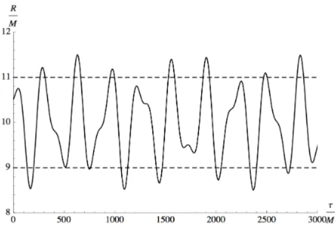
5.5.1 Planar orbits: double periodic, precession of periastron . . . . 72
5.5.2 Planar orbits: stability of circular orbits and the ISCO . . . 75
5.5.3 Non-planar orbits: Geodetic precession . . . 78
5.6 Circular motion: non-minimal gravitational Stern-Gerlach force . . . 79
6 Conclusion 85 A Deviation Equations in Schwarzschild space-time 87 A.1 The Orbital deviations: . . . 87
A.2 The spin-dipole deviations: . . . 88
Bibliography 91
Summary 101
Samenvatting 107
Publications 113
CONTENTS
Curriculum Vitae 115
Acknowledgements 117
List of Figures
Figure Page
1.1 Polarisation of gravitational waves . . . 9
1.2 Orbital decay of PSR B1913+16 . . . 10
1.3 Black Holes and Gravitational Waves . . . 11
1.4 GW150914 . . . 12
1.5 Coalescence of two supermassive black holes . . . 14
1.6 The Big Bang and The Early Universe . . . 14
1.7 Extreme Mass Ratio Systems . . . 14
3.1 Orbits of a test mass in the Schwarzschild space-time . . . 38
4.1 World-line of a spinning particle . . . 51
5.1 Radial deviation from circular orbit . . . 74
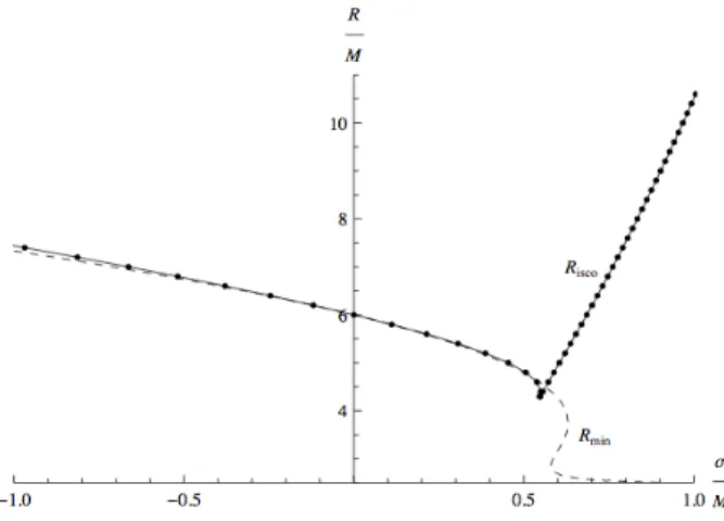
5.2 ISCO . . . 77
5.3 ISCO compared with minimal orbital angular momentum . . . 77
6.1 Circular orbit . . . 103
6.2 Periastron shift . . . 104
6.3 Geodetic Orbit . . . 105
6.4 Circulaire baan . . . 110
6.5 Periastronverschuiving . . . 110
6.6 Geodetische baan . . . 111
Overview
The gravitational two-body problem has been a subject of interest long before the origin of General Relativity. In Newtonian mechanics, an isolated system of two point particles interacting through gravity is readily solvable and the resulting motion is periodic. The energy and angular momentum are represented by two conserved integrals of motion. In General Relativity non-separable centre of mass co-ordinates require taking account of the internal structures of the bodies, and therefore it is extremely complicated. The problem has been investigated since the beginning of General Relativity through the pioneering works of Einstein, Lorentz, Droste and De Sitter. The equations of motion for comparable mass binaries have been computed with the Post-Newtonian expansion. Even after 100 years of Gen-eral Relativity the analysis is still incomplete. The Post-Newtonian description is sensible only in the weak field regime i.e., in-spiralling stage. When the two com-pact bodies are too close the gravity is so strong that the objects travel almost at the speed of light: the strong-field dynamical regime.
The dynamics of binaries is nonlinear in General Relativity and therefore the orbits are never periodic: as the system emits gravitational waves it continuously loses energy and angular momentum. Then the radiation back-reaction drives the objects closer and closer, eventually to merge. During the final stages of merger the analytical methods are ineffective and therefore the Numerical Relativistic treat-ment is used [1]. The reverse is also true; Numerical Relativistic methods are less efficient when the two objects are far apart, or when one of the components is much heavier than the other.
The latter type of system is known as theExtreme Mass Ratio System. Since the orbiting object is much smaller than the stable central one, the system can be analysed within the framework of black hole perturbation theory. If we neglect the internal structure and back reaction of the smaller compact object, we can treat it as a point particle moving on a world line, as described by Einstein [2] for test masses. In this limit many quantities which describe the evolution of the binaries can be solved quite precisely. Since all astrophysical objects spin, it is essential to include the internal angular momentum of compact objects. Such a
Overview
description of Extreme Mass Ratio binaries is important e.g. for low frequency space-based gravitational-wave detectors such as the evolved Laser Interferometer Space Antenna.
For more than eighty years, mathematical descriptions have aimed at keeping track of the centre of mass with various spin supplementary conditions; with the gravitating objects possessing quasi-rigid rotation along with orbital motion (ex-tended bodies), this defines the framework of the Mathisson-Papapetrou model. But in determining the overall motion of the body by following a detailed micro-scopic description of a material body is often too complicated and the correct spin supplementary condition is still in debate.
Therefore we have given a alternate complementary formalism to the subject. We construct effective equations of motion for point-like objects, which is an ideal-ization of a compact body, at the price of neglecting details of the internal structure by assigning the point-like object an overall position, momentum and spin. This is also known as the spinning-particle approximation, and is used for the semi-classical description of elementary particles as well. A detailed account on the qualitative connections and differences between the two formalisms have been given in section
4.4.
We have derived equations of motion for compact spinning bodies in curved space-time in an effective world-line formalism. The equations are obtained both from a hamiltonian formulation, without using any supplementary conditions and also from local energy-momentum conservation. The price to pay is that the world-line does not always coincide with that of a centre of mass but rather follows the spin, with the result that there is a mass dipole describing the displacement between the two in the presence of curvature. One of its strong points is that it does not require an a priori choice of hamiltonian. Since the closed set of Poisson-Dirac brackets is model independent, it can be applied to a large variety of models of relativistic spin dynamics. Using a minimal choice of hamiltonian we obtain the equations of motion by computing its bracket with this hamiltonian. The analysis has been extended with gravitational and electric Stern-Gerlach interactions by introducing the non-minimal hamiltonians. Also modified conservation laws emerge reflecting the spin-orbit coupling.
We have applied our formalism to study the dynamics of spinning particles in Schwarzschild space-time and established number of physical results. We obtain the simplest orbit: circular, for the particle in the equatorial plane. Method of geodesic deviation in General Relativity has been generalised to world lines of particles carrying spin. The complete first-order solution for the non-circular planar orbits are found starting from the circular orbit. The spin-influenced perturbations have double periods, and therefore the periastron and apastron behave in a complicated way (non-constant intervals) i.e., not only subject to an angular shift, but the point of closest approach shows radial variations as well. The presence of spin alters
Overview
the stability conditions and therefore the location of the Innermost Stable Circular Orbit. We have shown for over a wide range of spin values−0.5M < σ <0.5M, the Innermost Stable Circular Orbit is quite close to the orbit of minimal orbital angular momentum and coincides only for spineless particles. We have furthermore extended our analysis for a non-minimal hamiltonian to include Stern-Gerlach force of gravitational origin and determined circular orbits in the case of Schwarzschild. As a further generalisation we investigated non-planar eccentric orbits around a massive stable black hole. We have obtained an analytical formula for the orbital precession frequency.
1
Introduction
1.1
Gravitation
Of the four fundamental forces of nature, gravity is the weakest. For instance, the gravitational force between the proton and electron is1040 times smaller than the electric force that binds these particles together in atoms. However gravity is a universal force. Newton’s law of gravitation was the first major physical theory which attempts to describe gravity. According to Newton’s theory, two bodies, irrespective of whether they are on the Earth or in the heavens, whether they are in the state of motion or rest, always mutually attract each other with a force directly proportional to the product of their mass and inversely proportional to the square of their mutual distance
F =GmM
d2 , (1.1.1)
whereF is the force between the masses;Gis the universal gravitational constant, whose value is 6.674×10⁻¹¹N m2/kg2; m and M are two masses, and d is the distance between the centers of the masses. This implies, the gravitational force propagates in space at an infinitely great speed. This is the weak point of New-ton’s theory, because it means that something is simultaneously having an effect somewhere, where it is not present, and this is a physical impossibility. Despite this weakness, it still provides an excellent basis for explaining and calculating the planetary movements.
This absurd idea of "action at a distance" emerging in Newton’s theory was not resolved, until Einstein in 1915. Einstein described space and time as different aspects of reality in which matter and energy are ultimately the same. With this he describes gravitation very accurately in this 4-dimensional universe (3 spatial dimension + 1 time dimension) in which we are living in. The presence of large amounts of mass or energy distorts space-time – in essence causing the fabric to "warp" and we observe this as gravity.
Freely falling objects – whether a soccer ball, a satellite, or a beam of starlight – simply follow the shortest space-time path (geodesic) in this curved space-time.
1. Introduction
Therefore, the planets are moving in "straight lines" in the curvature produced by the sun and it appears as if they are in circular or elliptical motion around the sun. This is the central idea of general theory of relativity [3].
Thus the Newtonian idea of a gravitational force acting at a distance between bodies was replaced by the idea of a body moving in response to the curvature of space-time. Indeed Newton’s theory of gravity is not completely wrong. It is a correct approximation to Einstein’s theory when space-time curvature is negligible and the velocities of masses are much smaller than the velocity of light.
Newton’s theory forms an excellent basis for describing weak gravitational regimes like in earth or solar system. In this regimes the general relativistic cor-rections to the Newton’s theory are very small. But general relativity also predicts new strong gravitational phenomena like bending of light, black holes, gravitational waves and the big bang.
1.2
Gravitational Waves
Accelerated mass varies time and the change propagates as ripples in space-time curvature with the speed of light known as gravitational waves. Gravitational waves are analogous to the electromagnetic waves, the oscillations in the electric and magnetic fields produced by the accelerated charges.
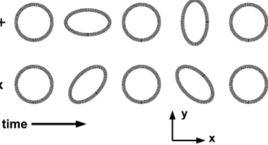
Mass in motion is the source of gravitational waves. In turn, gravitational waves can be detected through the motion of masses produced as the ripple in space-time curvature passes by. When a gravitational wave passes through a ring of particles it changes their relative positions, depending on the wave’s polarisation [4]. Here we have shown the particle’s motion produced by a wave with "+" polarisation (top line) and”×”polarisation (bottom line).
Fig.1.1implies that a single wave cycle of a gravitational wave changes the ring (R being the radius) into an ellipse with semi-major axisR+dR and semi-minor axis R−dR, back through a ring into the same ellipse rotated by90◦ and finally back to a ring. The strength of a gravitational wave is determined by how rapidly the quadrupole moment of its source is changing:
h' G
c4
d2Q/dt2
D (1.2.1)
where h is the strain, the strength of a gravitational wave, Q is the quadrupole moment of the source and D is the distance from source to observer and c is the speed of light.
In principle any accelerated mass produces gravitational waves, for example a falling apple. But the quantity cG4 = 8.26×10−
45kg−1(m/s2)−1 is very tiny, therefore we need very large masses undergoing extreme accelerations to produce detectable gravitational waves. Thus we look for most energetic phenomena in the universe like big bang, supernovae explosion or compact binary coalescence [5].
1.3. PSR B1913+16: Indirect Evidence of Gravitational Waves
Figure 1.1. The effect of a gravitational wave on a ring of particles. The wave is traveling in the z-direction (perpendicular to the page). The upper and lower parts are the effects of a "+" and”×”polarised wave, respectively.
1.3
PSR B1913+16: Indirect Evidence of Gravitational Waves
Even after several years of general relativistic predictions of gravitational waves, their existence was not universally believed. The very first convincing experimental evidence was given by Russell Hulse and Joseph Taylor in 1974 [6] in connection with the discovery of binary pulsar PSR B1913+16. The observed system must be composed of neutron stars, at least one of which is a pulsar. We observe a pulse of radio waves every time the bright spot sweeps around to face Earth [7]. The pulsar has a rotational period of 59 ms and its frequency varied with a period of 7.75 hours; apparently it is a member of a binary system with high eccentricity [8,9].
After several years of observation [10,11], a variety of relativistic effects has been recognized: orbital precession, advance of periastron, gravitational redshift, and the time-dilation and so on. It is found that both the objects in the system were neutron stars (incredibly dense objects the burned-out core often left behind after a supernovae) with masses around 1.4M (solar mass). But the most
excit-ing prediction was that they found the orbital period was decreasexcit-ing by about 75 millionths of a second per year. This could not be understood unless the dissipa-tive reaction force associated with gravitational waves produced is included. Thus the two neutron stars gradually fall closer to each other and their orbital speed increases steadily because it emits energy as gravitational waves and this is in ex-cellent agreement with the rate predicted by the general relativity as shown in the Fig.1.2.
The frequency of the gravitational waves from the Hulse-Taylor binary system are too low for the existing ground based detectors to detect the signal. But the rate of orbital decay as predicted by the general relativity is in perfect agreement with the experimental observation is the very first strong evidence for the existence of gravitational waves [12,13]. This discovery of Hulse and Taylor has opened a new window to study gravitation and they were awarded Nobel prize in 1993.
1. Introduction
Figure 1.2. The orbital period of binaries PSR B1913+16 decreases because the system loses energy as gravitational waves. Since the system is relativistic, the effect is very strong here. The measure of this decrease in orbital period is due to the steady shift over time of the time of the pulsar’s periastron (closest approach to its companion). The points are the observed data points over several decades and the solid line is the general relativity prediction.
1.4
GW150914: The Direct Detection of Gravitational Waves
According to general relativity, whenever a sufficient mass is compressed into a very small volume such that the gravitational pull at the surface is too large, even light cannot escape once it enters into the surface. Such objects are called black holes. Black holes can be identified with minimum number of properties like mass, spin and charge.
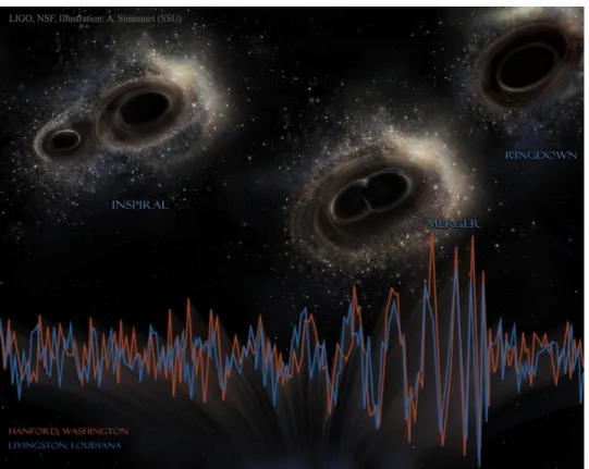
Coalescence of black hole binaries are the most promising sources of gravita-tional radiation [14,15]. According to general relativity the coalescence happens in three phases: in-spiral, merger and ringdown (Fig. 1.3). During the evolution there is loss in the energy and angular momentum of the system; as they are carried away by the gravitational waves. Therefore the orbit shrinks at the rate predicted by general relativity, and is already confirmed by the observation in the Hulse-Taylor binary system.
1.4. GW150914: The Direct Detection of Gravitational Waves
"The black holes of nature are the most perfect macroscopic objects there are in the universe: the only elements in their construction are our concepts of space and time. And since the general theory of relativity provides only a single unique family of solutions for their descriptions, they are the simplest objects as well."
–S. Chandrasekhar, The Mathematical Theory of Black Holes [16]
Figure 1.3. The evolution of binaries occur in three stages: in-spiral, merger and ring-down, as shown above. During the merger phase the system emits huge amount of grav-itational waves. The orange coloured wave is the gravgrav-itational wave pattern observed in LIGO - Hanford and similarly the blue coloured wave is the pattern obeserved in LIGO - Livingston. These observations are named as GW150914 to indicate that the gravita-tional waves passed the detectors on 2015 September 14 (EST). Credit: LIGO / NSF / A. Simonnet (SSU)
1. Introduction
After the completion of field equations in 1915, Einstein predicted the existence of gravitational waves in 1916. Historically searches for gravitational waves were started with the development of "Weber bar" detectors [17] and then Interferometric detectors since 1970 [18,19].
After five decades of work, advanced Laser Interferometer Gravitational-Wave Observatory (advanced LIGO) is in operation now and made thefirstdirect obser-vation of gravitational waves [20,21]. The event is named as GW150914 to indicate that the gravitational waves passed the detectors on 2015 September 14 (EST). The wave appeared first at Livingston, LIGO detector and then at Hanford, detector, a 7 ms later. This time difference is consistent with the fact thatgravitational wave travels at the speed of light. The gravitational wave stretched and squeezed space-time with the frequency sweeping from 40 Hz to 260 Hz over 0.2s in the pattern of two black holes merging together (Fig.1.4). The masses of two black holes are
Figure 1.4. Pictures from the paper [20] reporting the GW150914 discovery. The fre-quency of gravitational wave oscillation plotted vertical, as a function of time plotted horizontally. The colors show the strength of the waves. Green and yellow represents the oscillations of gravitational wave; yellow represents the very strong oscillations during the merger phase. Blue colour due to noise in the detector. At both Hanford and Livingston, the green-yellow oscillations have precisely the form that we expect for gravitational waves produced by binary black holes in-spiralling and colliding.
predicted to be 29Mand 36M. They merged to form a single black hole with a
mass of 62M. Thus the remaining 3M energy is released as gravitational waves
during the inspiral and merger phases of these black holes. Then the remnant black hole has spin at a rate of 100 rotations per second. Thus the discovery implies the following conclusions:
(i). First direct detection of gravitational waves
(ii). First direct evidence of existence of black holes
(iii). First observation of binary black holes.
1.5. Laser Interferometer Space Antenna (eLISA) and sources
This discovery give rise to a new branch of astrophysics: gravitational wave astron-omy [22,23]. Through which we can explore the dark side of the universe in the very broad spectrum which were inaccessible to us with electromagnetic astronomy. Black holes and/or neutron stars, composed of stellar mass binaries are opti-mistic sources for ground based network of detectors [24–27] like advanced-LIGO, VIRGO, KAGRA, GEO 600 and LIGO-India. The observation of gravitational waves from such binaries will bring various information: event rate, binary param-eters and even possible deviations from general relativity [28–30].
1.5
Laser Interferometer Space Antenna (eLISA) and sources
The existing ground based detectors are sensitive around 100 Hz. The universe is rich in strong sources of gravitational waves when we probe below these frequen-cies. But the seismic noise makes the ground based detectors insensitive for lower frequencies. Therefore we need observations from space. The space based detector eLISA is sensitive for frequencies from 0.1 mHz to 100 mHz [31,32], and it is planned to be launched by European Space Agency (ESA) in 2034. These frequencies cor-responds to wide range of gravitational wave sources and its direct detection with eLISA will answer the very fundamental questions; mapping the present universe to all the way shortly after the Big bang. The mission has been named with the science themeThe Gravitational Universe [33] by the ESA.
The electromagnetic observations clearly show that stars, black holes, and galaxies are ubiquitous components of the universe [34]. eLISA will study these objects in the gravitational wave spectrum. Thus it measures the amplitude of the strain in the space as a function of time. The following are the prospective sources (not limited to) of gravitational waves:
Supermassive Binary Black Holes Almost all bright galaxies (including our own Milky Way) host one or more massive central black holes. Their masses range from 104 M – 107 M and these are called as supermassive black holes. When
galaxies coalesce (Fig. 1.5), these black holes will merge eventually [35], releasing huge amount of gravitational radiation during the process. Thus detecting these signals will not only test theories of gravity and black holes, but also reveal infor-mation about the evolution and merger history of galaxies [36].
Ultra-Compact Binaries The components of binaries could be compact objects like stellar mass black holes, neutron star or white dwarf. The Milky Way is full of these sources [37], but only a small fraction is observable in the radio and X-ray spectrum. Since the maximum loss of energy from these systems are always through gravitational waves, and it lies in the frequency range of eLISA [38], it should be possible to map all these objects soon.
1. Introduction
Figure 1.5. Coalescence of two super-massive black holes. The expected grav-itational waveform has in-spiral, merger and ringdown phase. Merging galaxy NGC 6240 [35] has two giant black holes as re-ported by NASA’s Chandra X-ray observa-tory. Credit: NASA / ESA / the Hubble heritage / A. Evans.
Figure 1.6. The fossil gravitational waves are the only way to probe the early Uni-verse all the way immediately after the Big Bang. The expected gravitational waveform is stochastic background (ran-dom noise). Credit: NASA / WMAP sci-ence team.
Figure 1.7. An artist impression of EMRS; a small black hole inspiralling around a supermassive black hole. The modelled waveform would have many har-monics as shown. Credit: NASA.
1.5. Laser Interferometer Space Antenna (eLISA) and sources
The Big Bang and The Early Universe Since the universe was transparent to gravity moments after the Big Bang and long before light (remember the first light still present, Cosmic Microwave Background was produced only about 300,000 years after the Big Bang), gravitational waves will allow us to observe further back into the history of the universe than ever before. And since gravitational waves are not absorbed or reflected by the matter in the rest of the universe, we will be able to see them in the form in which they were created. Immediately after the Big Bang, when the Universe was very young it underwent a period of very rapid expansion, as a result space-time got distorted which in turn produced gravitational waves between approximately10−43to10−32seconds after the Big Bang (Fig.1.6). These relic gravitational waves from the early evolution of the universe may carry information about the origin and history of the universe.
Extreme Mass Ratio Systems The supermassive black holes in the galactic centres may be accompanied by one or more stellar mass compact objects like black hole, neutron star or white dwarf, of few solar masses are called Extreme Mass Ratio Systems (EMRS) (Fig.1.7). eLISA will track the complex relativistic orbits of the stellar companion around a central black hole in the mass interval between104M
< M <5×10⁶M
for upto104 –105cycles [39,40]. The waveforms emitted from
these systems would inform us about the stellar mass compact object populations, mass spectrum and their spin. It will also describe the properties of space-time geometry around the central black hole [41,42] and the formation of supermassive black holes at the galactic centers [43].
Infrared astronomy has given thebest empirical evidence for the existence of a 4 million solar mass black hole in our Milky Way. Observation has not only tracked the 28 stars orbiting a supermassive black hole [44,45]: Sagittarius A*, but also predicted its mass and distance (27,000 light years away from the solar system). The stellar orbits in the galactic centre show that the central mass concentration of four million solar masses must be a black hole, beyond any reasonable doubt [46].
Though most of the black holes in nature are spinning, we start modelling EMRS as a small spinning black hole or a neutron star orbiting around a static spherically symmetric - supermassive black hole. This is the subject of this thesis. The mass ratio between the smaller compact object and the central black hole is typically∼10−5. Because of this extreme mass ratio, the curvature produced by the smaller object can be neglected. I introduce the necessary general relativistic tools for modelling EMRS in chapter 2 & 3. After this I discuss EMRS: a test mass orbiting a Schwarzschild black hole in chapter 3. Then I discuss the formalism for a spinning compact object in Schwarzschild space-time in chapter 4, which we have developed recently [47]. In chapter 5, I discuss the applications of our formalism and important aspects of the dynamics of EMRS [48]. The theoretical model I present in the rest of the thesis is esentially the preparation for eLISA observations. The
1. Introduction
first direct observation of EMRS and therefore supermassive black holes, through gravitational wave detection is expected immediately after the launch of eLISA mission. The estimated detection rates based on the best available models are 50 events for a 2 year mission [49].
2
Gravity and General Relativity
2.1
The Equivalence Principle
The Equivalence Principle is a corner stone of Einstein’s theory of gravity, General Relativity (GR) [50].
In its original form it refers to the equivalence between gravitational and iner-tial mass, as demonstrated experimentally by various scientists from the late 16th century onward. This was the starting point for Newton’s theory of gravity in which the gravitational pull of the earth gives the same acceleration to an apple and to the moon. In GR it holds as the acceleration of objects results from the geometry of space-time, independent of mass or composition. In this context it is usually referred to as theWeak Equivalence Principle.
The Equivalence Principle formulated by Einstein, the Einstein Equivalence Principleis slightly stronger. It says that a reference system in free fall is a local Lorentz frame, in which the laws of special relativity hold. In such a system non-interacting objects fall at the same rate with no relative acceleration. It is alocal
Lorentz frame as these statements only hold in the limit that distances are small compared to the local scale of space-time curvature, otherwise there would be tidal accelerations.
There also exists a third version of the Equivalence Principle, which states that the equivalence of gravitational and inertial mass includes all possible contributions to the mass including gravitational binding energy (self-energy). This is called the
Strong Equivalence Principleand is most difficult to test, as usually gravitational binding energy is extremely weak. The only objects in which gravitational con-tribution to mass is significant are compact bodies like neutron stars and black holes.
2. Gravity and General Relativity
2.2
Coordinates, metric and motion
In the absence of gravity, in a local Lorentz frame, free particles move with constant velocities on straight trajectories. When different sections of these trajectories in overlapping Lorentz frames are glued together, one gets trajectories which are still in a generalized sense the "shortest path" between two space-time points: geodesics
[51].
An invariant measure of distance along a particle’s space-time trajectory, or
world line, is the proper timeτ. It is the time measured during any short sections of the worldline by a clock at rest w.r.t. the particle. Let(x) be a coordinates for the patch of space-time where the trajectory is located, and consider two points on the trajectory with coordinates(xµ)and(xµ+dxµ). Then the proper time interval
dτ is determined from a quadratic expression in the coordinate intervalsdxµ:
−dτ2=gµν(x)dxµdxν. (2.2.1)
The coefficientsgµν(x)define the metric for the coordinate systemxµ at the given point. As it is an invariant, the same quantity measured in terms of a different coordinate system(x0)is
−dτ2=gµν0 (x0)dx0µdx0ν. (2.2.2)
Now the diffeomorphism xµ → x0µ(x) if it is smooth allows us to write the last expression also as
g0µν(x0)
∂x0µ ∂xκ
∂x0ν ∂xλ dx
κdxλ. (2.2.3)
Comparing with expression (2.2.1) gives
gκλ(x) =gµν0 (x0)
∂x0µ
∂xκ
∂x0ν
∂xλ. (2.2.4)
This shows how the metric coefficients change between different coordinate systems. The inverse metric is written gµν(x), such that at the same point in the same coordinate system
gµλgλν =δνµ.
It changes between coordinate systems by the inverse transformation
gµν(x) =g0κλ(x0)∂x
µ
∂x0κ
∂xν
∂x0λ.
Now the total proper time along a curvexµ(τ)between two space-time points(a, b) with time-like separation is
Z b
a
dτ. (2.2.5)
2.3. Hamiltonian dynamics
Notice that we can introduce an arbitrary parameterλ labeling the points on the curve, as long as it is monotonic between(a, b). Therefore, the time interval
dτ =
−gµν
dxµ
dλ dxν
dλ
1/2
dλ, (2.2.6)
wheredλis the displacement on space-time. We are varying the paths
xµ(x)→xµ(x) +δxµ(x) (2.2.7) keeping the end-points fixed, and will denote theτ-derivatives by x(τ)˙ and ∂λ ≡
∂
∂xλ =,λ. By the standard variational procedure one then finds
δS = 1 2
Z
dλ
−gµν
dxµ
dλ dxν
dλ
−1/2
−δgµν
dxµ
dλ dxν
dλ −2gµν dδxµ dλ dxν dλ = 1 2 Z dτ
−gµν,λ x˙µx˙νδxλ+ 2gµνx¨νδxµ+ 2gµν,λx˙λx˙νδxµ
=
Z
dτ
gµν¨xν+
1
2(gµν,λ+gµλ,ν−gνλ,µ) ˙x
ν ˙ xλ δxµ (2.2.8)
Here the factor of 2 in the first equality is a consequence of the symmetry of the metric, the second equality follows from an integration by parts, the third from relabelling the indices in one term and using the symmetry in the indices ofx˙λx˙ν in the other.
We set the variation of action to zero,δS = 0. Further re-naming µ→κand multiplying bygµκ, we obtain the equations for a timelike geodesic in an arbitrary gravitational field:
d2xµ
dτ2 + Γ
µ νλ
dxν
dτ dxλ
dτ = 0, (2.2.9)
whereΓµνλ is the Christoffel connection or Levi-Civita symbol, which is symmetric in the second and third indices:
Γµλν = Γµνλ=1 2g
µκ(g
κλ,ν+gκν,λ−gλν,κ). (2.2.10)
2.3
Hamiltonian dynamics
The equation (2.2.9) for geodesic motion was derived from the geometric princi-ple of extremizing the amount of proper time along the curve. However the same equation of motion can also be obtained in a canonical phase-space approach with an appropriate hamiltonian. This approach introduces next to the particle’s co-ordinates xµ(τ) also the canonical momenta π
µ(τ). The appropriate hamiltonian is
H = 1 2mg
µν(x)π
µπν. (2.3.1)
2. Gravity and General Relativity
Hamilton’s equations then imply the following equations of motion:
˙
xµ= ∂H ∂πµ
= 1 mg
µνπ ν,
˙ πµ=−
∂H ∂xµ =
1 mgκλ,µg
κρgλσπ
ρπσ=mgκλ,µx˙κx˙λ.
(2.3.2)
These equations can be rewritten in the form
πµ=mgµνx˙ν, x¨µ+ Γµλνx˙
λx˙ν = 0. (2.3.3)
Thus equation (2.2.9) is reobtained. Although less geometric, this method is entirely equivalent and is useful if more interactions than just with the curved background geometry are to be included, like electric charge or spin. This will become clear in the chapters to follow.
2.4
Differential geometry
The quantities that appeared in the previous sections can be introduced in a more general way not only on curves (geodesics) but as fields of geometric objects on the space-time manifold at large [52]. Vector fields Aµ(x) are sets of functions transforming under a change of coordinates as
Aµ(x) =A0ν(x
0)∂x0ν ∂xµ,
and similarly for higher-rank tensors Aµν.... Taking the derivative of a vector or tensor is somewhat delicate, as in general it produces an new object which is not a tensor itself. However, one can define acovariantderivative using the Christoffel connection introduced before. Indeed one can construct a proper rank-2 tensor from a vector by taking
DλAµ=∂λAµ−ΓνλµAν. (2.4.1)
Similarly a rank-2 tensor is lifted to a rank-3 tensor by taking
DλAµν =∂λAµν −ΓκλµAκν−ΓκλνAµκ,
etc. To prove the statement one has to check the transformation properties of the connection coefficients:
Γµλν(x) = Γ0ρσκ(x0)∂x 0ρ
∂xλ
∂x0σ ∂xν
∂xµ ∂x0κ −
∂2x0κ ∂xλ∂xν
∂xµ ∂x0κ.
For proofs we refer to the literature [3,50].
2.4. Differential geometry
Clearly in contrast to ordinary partial derivatives, covariant derivatives do not commute. Indeed
[Dµ,Dν]Vλ =Dµ(∂νVλ−Γ ρ
νλVρ)−(µ↔ν)
=∂µ(∂νVλ−ΓρνλVρ)−Γσµν(∂σVλ−ΓρσλVρ)−Γσµλ(∂νVσ−ΓρνσVρ)
−(µ↔ν)
=−∂µ(ΓρνλVρ)−Γσµλ(∂νVσ−ΓρνσVρ)−(µ↔ν)
=−∂µΓ ρ
νλVρ+ ΓσµλΓ ρ
νσVρ−(µ↔ν)
=RµνλρVρ
(2.4.2) where
Rµνλρ=−∂µΓρνλ+∂νΓρµλ−ΓσνλΓ ρ
µσ+ Γ
σ µλΓ
ρ
νσ. (2.4.3)
Here although each single term inRµνλρis not a tensor, under a diffeomorphsim, we can prove the following transformation properties [3] for the resulting combination
R0σαξβ= ∂x
µ
∂x0σ
∂xν ∂x0α
∂xλ ∂x0ξ
∂x0β ∂xρ R
ρ
µνλ , (2.4.4)
and therefore, it is a (1, 3)-tensor; called as theRiemann tensor. It includes second-order derivatives of the metric: it does not vanish therefore in a locally inertial frame. It vanishes if and only if a manifold is flat. It is therefore the curvature tensor. In particular, if the Riemann tensor vanishes, we can always construct a coordinate system in which the metric components are constant.
The Riemann tensor (2.4.3) satisfies a number of symmetry properties. It is anti-symmetric in the first two or last two indices and symmetric in the first and last pairs of indices:
Rµνρσ=−Rµνσρ, Rµνρσ=−Rνµρσ, Rµνρσ =Rρσµν, (2.4.5)
and sum of cyclic permutation are zero:
Rµνρσ+Rµρσν+Rµσνρ= 0, (2.4.6)
where the first index has been lowered using the metric: Rµνρσ = gµηRηνρσ. It can be shown that these constraints reduce the number of independent components of the Riemann tensor in n dimensions from n4 to n2 n2−1
/12, i.e. 20 in 4 dimensions, and only 1 in two dimensions.
2. Gravity and General Relativity
Then the invariant parts of the Riemann tensor are defined as the Ricci tensor (a symmetric tensor)Rµν and Ricci or curvature scalarR:
Rµν ≡Rαµαν, R≡gµνRµν. (2.4.7)
In addition to these algebraic identities, the Riemann tensor obeys a differential identity:
∇γRµνρσ+∇σRµνγρ+∇ρRµνσγ= 0, (2.4.8)
also called as Bianchi identity. Further contracting the Bianchi identity gives
∇µR
µν =
1
2∇νR. (2.4.9)
This allows to define a "conserved" tensor, theEinstein tensor:
Gµν =Rµν−
1
2gµνR, (2.4.10)
i.e., the Bianchi identity implies that the divergence of this tensor vanishes identi-cally,
∇µGµν = 0. (2.4.11)
This is sometimes called the contracted Bianchi identity.
2.5
Einstein’s Field Equation
Einstein field equations [3,53] describe the physical universe as a 4-dimensional Lorentzian manifold. It is the relation between curvature and energy-momentum content in the universe. This allows us to view the curvature tensor as a physical property of the universe, as a function of mass, momentum and energy.
The curvature of the Lorentzian manifold of space-time is caused by energy-momentum. Since geodesics on this manifold are motions of particles in free fall; that is, only affected by the force of gravity, curvature and gravitation are linked. The source of gravity is energy-momentum, and the source of curvature in this manifold is gravity. The precise equation for this relation is formulated as
Rµν−
1
2gµνR=−
8πGTµν
c4 , (2.5.1)
where the left hand side is the Einstein tensorGµν as we defined in (2.4.10),G=
6.674×10⁻¹¹N m2/kg2 is the Newton’s constant,c=3×10⁸ is the speed of light andTµν is theEnergy-momentum tensor of all gravitating matter.
Now, number of observations can be made: As a consequence of Bianchi iden-tity, the Einstein’s tensor is covariantly conserved as shown in (2.4.11). Then the
2.5. Einstein’s Field Equation
consistency of the Einstein’s field equation (2.5.1) implies that the Energy momen-tum tensorTµν must also be covariantly conserved,
∇µT
µν = 0. (2.5.2)
Einstein’s field equations constitutes a set of non-linear coupled partial differential equations whose general solution is not known. Usually one makes some assump-tions, for instance spherical symmetry. Because the Ricci tensor is symmetric, the Einstein’s field equations constitute a set of 10 algebraically independent second order differential equations forgµν. Then the general covariant nature of Einstein equations makes us to expect only 6 independent equations for the metric.
Observe that the Riemann curvature tensor (2.4.3) contains terms, which are of the form a single derivative acting on the Christoffel connection, and terms which are quadratic forms in the connection. The Christoffel connection (2.2.10) is in turn expressed in terms of single derivatives acting on the metric tensor. This then implies that the Einstein’s field equation (2.5.1) contains derivatives of the metric tensor up to second order in space-time, and in that sense it resembles the Maxwell equations.
The principal difference between the electrodynamics and the dynamics of grav-itational field in GR are the nonlinear terms, contained in the quadratic forms in the Christoffel connection, which makes the theory more complicated. These terms are dynamically very relevant in strong gravitational fields. A second difference is that, in GR the dynamical field is the metric tensor, which is a rank two symmetric tensor field, while in the electrodynamics there are vector fields.
Finally, the coupling constant, 8πG/c4 ∼2×10−43s2kg−1m−1 is dimension-full, but extremely small on any other physical scale, such that only in the presence of matter under extreme conditions (large energy densities), the matter effects on space-time can be strong. Such extreme conditions are found in compact objects like black holes and neutron stars.
Thus, GR models the effects of gravity as the curvature of Lorentzian manifold. It of course also generalizes the special relativity by using an in general non-flat metric tensor, and in fact is required to approximate to special relativity locally. Special relativity is a special case of GR, where there is no gravitational force acting on the particle. Further, when the motion is non-relativistic and in the weak gravitational field, we can recover Newton’s theory of gravity: ∇2φ= 4πGρ(φ is the gravitational potential andρis the matter density).
3
Motion in Curved Space-time
3.1
Hamiltonian Formalism
The basic machinery of GR has been described in the previous chapter. Now we want to investigate the dynamics of test particles in curved space-time with in the Hamiltonian framework. Hamiltonian formalism includes three sets of ingredients: equations of motion, phase-space and the conserved quantities.
The equations describe test particle dynamics are so-called geodesic equations. We have derived geodesic equations of motion starting from the standard variational procedure and also from the Hamiltonian dynamics. In the following sections it is further shown that, it can be obtained from the principles of energy-momentum conservation.
The phase-space formulation of motion in curved space-time is being con-structed with the closed set of covariant Poisson-Dirac brackets, obeying Jacobi identities. It consists of the position co-ordinatexµ and the covariant momentum
πµ, and therefore its anti-symmetric bracket is:
{xµ, πν}=δνµ, (3.1.1)
all other possible brackets vanish. These brackets are independent of the specific Hamiltonian. Therefore, in principle we can use varieties of covariant Hamiltonians with the brackets to obtain the equation of motion. However, here we are interested in studying the geodesic motion of the test particle in curved space-time i.e., the particle’s interaction is strictly gravitational. Therefore as described in the previous chapter the appropriate Hamiltonian is
H = 1 2mg
µν(x)π
µπν. (3.1.2)
Then the proper-time evolution equations for phase-space co-ordinates are obviously generated by computing the brackets. It is important to note that this Hamiltonian describes the particle’s mass as a universal constant of motion for any space-time:
H =−m
2 ⇒ gµνu
µuν=−1. (3.1.3)
3. Motion in Curved Space-time
It is called the Hamiltonian constraint in the literature.
3.2
Symmetries, Killing vectors, and Constants of motion
In addition to the universal constants of motion eq. (3.1.3), there exists conserved quantities as a result of symmetries of space-time. Emmy Noether discovered that physical quantities such as energy, momentum, angular momentum, etc. which remain constant during the evolution of the system are related to symmetries of the dynamics. Thus symmetries lead to conservation laws, and knowing a conserved quantity of a dynamical system allows to reduce the dimension of the phase space in which the system is defined.
From special theory of relativity we know that suitable coordinate transforma-tions on the Minkowski metric leaves the metric invariant, giving rise to the Poincar´e group of symmetries. Similarly, the standard metrics on the two- or three-sphere have rotational symmetries because they are invariant under rotations of the sphere. We can describe this in two ways: either as an active transformation, in which we rotate the sphere and nothing changes, or as a passive transformation, in which we do not move the sphere, and we just rotate the coordinate system. These descrip-tions are equivalent.
In the context of geometry we definesymmetry as an invariance of the metric under a coordinate transformation. The symmetries of a metric are called isome-tries. Quantitatively, we start with a manifold M, with coordinates xµ. Let the metric in these coordinates begµν(x). Suppose we make an infinitesimal change of coordinates
xµ→x0µ=xµ−ξµ(x) (3.2.1) For detecting continuous symmetries we require the invariance of the line element under infinitesimal transformations. We know that the metric tensor transforms as
g0µν(x0) = ∂x
α
∂x0µ
∂xβ
∂x0νgαβ(x). (3.2.2)
Using the invariance of the metric under an isometry we can also write
g0µν(x0) =gµν(x0)'gµν(x)−ξλ∂λgµν(x). (3.2.3)
The infinitesimal coordinate transformation also implies
∂xα
∂x0µ 'δ α
µ+∂αξµ,
∂xβ
∂x0ν 'δ β
ν +∂αξν. (3.2.4)
Combining these results the Lie derivative of the metric w.r.t. the displacement vectorξµ must vanish:
Lξgµν ≡ξλ∂λgµν+∂µξλgλν+∂νξλgµλ= 0. (3.2.5)
3.2. Symmetries, Killing vectors, and Constants of motion
Using the metric postulate
∇λgµν = 0, (3.2.6)
this can be rewritten covariantly as
Lgµν =∇µξν+∇νξµ= 0. (3.2.7)
Vector fields satisfying these equations are called theKilling vectors. Now we will establish the conserved quantities associated with these Killing vectors.
3.2.1 Constants of motion
In classical mechanics, the angular momentum of a particle moving in a rotationally symmetric gravitational field is conserved. In GR the concept of symmetries of a newtonian gravitational field is replaced by symmetries of the metric, and we therefore expect conserved quantities associated with the presence of Killing vectors. Let us consider a massive particle moving along a geodesic of a spacetime which admits a Killing vectorξα. The geodesic equations written in terms of the particle’s four-velocityuα=dxα/dτ read
duα
dτ + Γ
α βνu
βuν= 0, (3.2.8)
by contracting the above equation withξα, we find
ξα
duα
dτ + Γ
α βνu
βuν
≡ d(ξαu
α)
dτ −u
αdξα
dτ + Γ
α βνu
βuνξ
α= 0 (3.2.9)
Since
uαdξα dτ =u
βuν∂ξβ
∂xν (3.2.10)
therefore eq. (3.2.9) becomes,
d(ξαuα)
dτ −u
βuν
∂ξ
β
∂xν −Γ α βνξα
≡ d(ξαu
α)
dτ −u
βuνξ
β;ν = 0. (3.2.11)
Sinceξβ;ν is antisymmetric inβandν, whileuβuν is symmetric, the termuβuνξβ;ν vanishes, and eq. (3.2.11) finally becomes
d(ξαuα)
dτ = 0 ⇒ ξαu
α=g
αµξµuα=const. (3.2.12)
Eq. (3.2.12) can re-written asξµπ
µ =constant≡J (let’s say), whereπµ=mgµνuν. It is also straight forward to check the quantityJis a constant of the particle motion, by demanding its brackets to vanish with the Hamiltonian:
{J, H}= 0 ⇒ Ji=ξiµπµ (3.2.13)
Thus, for every Killing vector there exists an associated conserved quantity.
3. Motion in Curved Space-time
3.3
Spherical symmetry
The Einstein Field Equations are a complicated set of non-linear equations with 10 unknown functions of space-time. These equations are most easily solved in space-times with a maximal number of symmetries as these give rise to a maximal number of constants of motion. This accessibility makes using spherically symmetric spacetimes all the more attractive as a starting point. Birkhoff’s theorem classifies all vacuum spherically symmetric spacetimes.
A spacetime is spherically symmetric if it admits an SO(3) group of isometries. In particular every point will lie on some round sphere, on which the rotation group acts transitively, which means that one can go from any point on the sphere to any other point by means of a rotation. Further a space-time is said to be stationary or static, if it exhibits the property of time-translation symmetry. Static spherically symmetric metrics admit four Killing vectors, one of which is timelike, while the remaining three are spacelike, representing the Lie algebra of the rotation group SO(3).
The most general, static and spherically symmetric metric can be expressed in spherical polar coordinates with the ansatz [16]
ds2=−f(r)dt2+g(r)dr2+r2 dθ2+sin2θdϕ2
. (3.3.1)
The coefficients f(r) and g(r) are fixed by requiring the asymptotic limit i.e., for
r→ ∞, the metric should be Minkowskian: ds2=−dt2+dr2+r2 dθ2+sin2θdϕ2
.
Due to isotopy and time independence these coefficients cannot depend on(t, θ, ϕ)
and no linear terms indθanddϕ.
Note that this metric is diagonal. Therefore the metric and its inverse has the following components only
gtt=−f(r) grr=g(r) gθθ=r2 gϕϕ=r2sin2θ
gtt=− 1
f(r) g
rr = 1
g(r) g
θθ= 1
r2 g
ϕϕ= 1
r2sin2θ.
(3.3.2)
The next steps are standard, we first compute the non-vanishing components of affine connectionsΓµλν= Γµνλ= 12gµκ(gκλ,ν+gκν,λ−gλν,κ):
Γttr= Γtrt =1 2 f0 f Γ r tt= 1 2 f0 g Γ r rr = 1 2 g0 g
Γθrθ= Γθθr=1
r Γ
r
θθ=−
r
g Γ
r
ϕϕ=−
r gsin
2θ
Γϕrϕ= Γϕϕr= 1
r Γ
ϕ
θϕ= Γ
ϕ
ϕθ=cot θ Γ θ
ϕϕ=−sin θ cos θ.
(3.3.3)
3.3. Spherical symmetry
where0 stands for ∂r∂ . Then the Riemann tensor contracted to get Ricci tensor
Rµν=∂νΓρρµ−∂ρΓρµν+ Γ σ ρµΓ
ρ
νσ−Γ
σ µνΓ
ρ
ρσ, (3.3.4)
and as a result
Rtt=
1 2 f00 g + 1 4
f02
f g − 1 4
f0g0 g2 +
1 2r
f0 g
Rrr =
1 2 f00 f + 1 4
f02 f2 −
1 4
f0g0 f g +
1 2r
g0 g
Rθθ=−1 +
1 g + r 2g f0 f − g0 g
Rϕϕ=sin2θ Rθθ
(3.3.5)
The non-diagonal componentsRµν withµ6=ν vanish. These geometric quantities are more general. Therefore it can be used for any static spherically symmetric space-time like Schwarzschild, Reissner-Nordstrøm etc.
3.3.1 The Schwarzschild solution
We now want to find an exact solution of Einstein’s equations in vacuumRµν = 0 (forµ6=ν), which is spherically symmetric and static. This will be the relativistic generalization of the newtonian solution for a pointlike massϕ=−M/rand it will describe the gravitational field in the exterior of a non-rotating body. The solution will be obviously in the form of eq. (3.3.1), where the coefficientsf andg are fixed in the following way:
The linear combination of time and radial equations of Ricci tensor implies
Rtt f + Rrr g = 1 r g0 g2 +
1 r
f0
gf = 0, (3.3.6)
which reveals a simple relation betweenf andg:
g0 g =−
f0
f ⇒ log(g) =−log(f) +constant, or g∝ 1
f. (3.3.7)
Now, we fix the proportionality constant betweenf and g as follows. Imagine we are extremely far away from the star (for example), then the metric should reduce to the Minkowski metric. So in the limitr→ ∞we have g=f = 1. This fixes the proportionality constant to be 1. Thereforeg= 1/f.
Then we only need to compute one of them from one of the differential equations (3.3.5). Let’s considerRθθ component and replaceg with1/f. We have
Rθθ= 1−rf0−f = 0 ⇒ f(r) = 1 +
C
r, (3.3.8)
3. Motion in Curved Space-time
where C is some constant we want to determine. We can fix the constant by resorting to the weak-field limit which should reproduce the Newtonian gravitational potentialϕ. In the weak-field limit we just have
f(r) = 1 + 2ϕ(r), where ϕ=−M
r , (3.3.9)
so the constantC=−2M. Then the complete line element in Droste co-ordinates; withM the mass,r the radius of the object,
ds2=−
1−2M
r
dt2+
1−2M
r
−1
dr2+r2 dθ2+sin2θdϕ2
. (3.3.10)
This is the famousSchwarzschild metric: a unique, static and spherically symmetric vacuum solution, according to Birkhoff’s theorem; obtained by the astronomer Karl Schwarzschild [54] in 1916, the very same year that Einstein published his field equations. It was apparently discovered independently by Johannes Droste [55], a student of Lorentz at Leiden University, around the same time.
The Schwarzschild metric (3.3.10) looks divergent atr= 2M, theSchwarzschild radius. As can be seen by switching to other ordinates this is actually a co-ordinate singularity, not a physical singularity of space-time. But the Schwarzschild radius defines a characteristic gravitational scale for any celestial object, related to the formation of a horizon. For the earth or even for the sun the radius is actually very smaller than the radius of the object itself. To compute the radius we need to insertGandc back to the expression and find
Rs=
2GM
c2 (3.3.11)
which is about 3km for the sun. So, for most astronomical objects this number is so small that we don’t need to consider it. However, objects smaller than their Schwarzschild radius disappear behind the horizon and become black holes.
3.3.2 Geodesic equations of motion and effective potential
We now want to consider the motion of a freely falling particle in the Schwarzschild space-time. The analysis can be simplified by using the constants of motion as im-plied by the Noether’s theorem; because of the spherical symmetry of the Schwarz-schild metric, there exists four constants associated with the Killing vectors (3.2.13):
Ji=ξiµπµ. Then
E=ξ0π0, Jj=ξjαπα (3.3.12)
where E is the particle’s energy;Jj = (J1, J2, J3)is the total angular momentum of the system. Without loss of generality we can choose the coordinate system such that θ =π/2 ⇒ uθ = 0, this way the trajectory lies on the plane perpendicular
3.3. Spherical symmetry
to the orbital angular momentum. Here the total angular momentum is strictly orbital, and the direction chosen to be z-axis. Then we write the equations of motion (3.2.8) in the component form [56]:
dut
dτ =− 2M r(r−2M)u
r
ut,
(3.3.13)
dur
dτ =−
M(r−2M) r3 u
t2+ M
r(r−2M)u
r2+ (r−2M)uϕ2,
(3.3.14)
duϕ
dτ =− 2 ru
ruϕ. (3.3.15)
Withz-axis being the choice of the angular momentum, the constants J1 and J2 turns out to be zero i.e., J1 =J2 = 0. Then we are left with the remaining two constants from (3.3.12); ε = E/m energy per unit mass and ` = J3/m angular momentum per unit mass,
ε=
1−2M
r
ut, `=r2sin2θ uϕ=r2uϕ. (3.3.16)
To establish the particle’s orbits, we investigate the equations (3.3.13), (3.3.14) and (3.3.15). Eq. (3.3.13) can be re-written as
d dτ
ln(ut) +ln
1−2M
r
= 0, (3.3.17)
which can be integrated asln
ut 1−2M r
=constant or
ut
1−2M
r
=constant (3.3.18)
Similarly eq. (3.3.15) is re-written as
1 r2
d dτ r
2uϕ
= 0, ⇒ r2uϕ=constant. (3.3.19)
From the Killing constants (3.3.16), we interpret (3.3.18) and (3.3.19) asε and`. This implies geodesic equations (3.3.13) and (3.3.15) doesn’t give any new result. Thus we are left with the radial geodesic equation (3.3.14) only. Upon using the Killing constants (3.3.16) forutanduϕ, it turns out be
dur dτ =−
M ε2 r(r−2M)+
M r(r−2M)u
r2+` 2
r4(r−2M). (3.3.20)
3. Motion in Curved Space-time
a relation for (ε, `). A second relation between these quantities are given by the Hamiltonian constraint: gµνuµuν = −1, similarly by using the Killing constants (3.3.16) we express
1−2M
r
ut2− u
r2
1−2M r
−r2uϕ2= 1 ⇒ ur2+
1−2M
r ∆ + l2
r2
=ε2.
(3.3.21) or
E=1 2u
r2+1
2
1−2M
r ∆ + l2 r2 −1 (3.3.22)
where,E= (ε2−1)/2is the total energy. Note,∆ is1for massive particles and0 for massless particles. If the particle is massless, the geodesic equation cannot be parametrized with the proper time. In this case the particle worldline has to be parametrized using an affine parameterλsuch that the geodesic equation takes the form (3.2.8), and the particle tangent vector isuα=dxα/dλ. The derivation of the constants of motion associated to a spacetime symmetry, i.e. to a Killing vector, is similar as for massive particles, recalling that by a suitable choice of the parameter along the geodesic J = {E, Ji}. Then since for massless particles m2 = 0, the Killing constantsεand`are identified as energy and angular momentum.
Eq. (3.3.22) has the form of an energy equation with a "kinetic energy" term,
˙
r2 plus a function of r, "potential energy" equalling a constant. Thus the motion in the radial coordinate is exactly equivalent to a particle moving in an effective potentialVef f(r)where
Vef f(r) =
1 2
1−2M
r ∆ + l2 r2 −1 . (3.3.23)
Then the simplest orbits one can start with are circular orbits i.e.,r=R, for which we can differentiate the potential and set it to zero: ∂rVef f(r) = 0,which results:
`2(R−3M) = ∆M R2 (3.3.24)
Thus we conclude, the circular geodesics exists only for R > 3M, for massive particles (∆ = 1) andR = 3M implies null geodesic which is interpreted as light ring for massless particles (∆ = 0). Further evaluating the second derivative of the potential yields
∂2Vef f(r)
∂r2 = 2∆
M R3
(R−6M)
(R−3M) (3.3.25)
we observe the circular orbits forR≥6M are stable and positive;R= 6M implies the flex point. Then the circular orbits between the radius 3M ≤ R < 6M are necessarily unstable.
3.3. Spherical symmetry
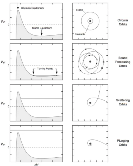
We show the above results qualitatively in Fig.3.1[50]. Massive test particles obey four kinds of orbits in Schwarzschild space-time. The Schwarzschild potential has one maximum and one minimum if`/M >12. The following 4 points describes the Fig.3.1from the top:
(i). The circular orbits exists at the radii, when the potential has minimum or maximum. The orbit at maximum will be in unstable equilibrium, because a small perturbation will through the particle to infinity or the particle will reach the singularity atr= 0.
(ii). For E < 0, the particle bounds between two turning points. The cross symbols are the turning points: the closest approach to the centre is the perihelion and the farthest approach is the aphelion.
(iii). WhenEis positive and less than the maximum of the effective potential, then the orbit is scattering. That is the particle comes from infinity and orbits the centre and then moves out to infinity.
(iv). IfE is greater than the maximum, then the particle comes from infinity and plunges into the centre.
Now re-writing eq. (3.3.24) forR results,
R= `
2
2M 1 +
r
1−12M
2
`2
!
(3.3.26)
which relates the radius of the orbits to angular momentum per unit mass`. Thus the minima of the potential lies at a special value of `= 2√3M, called as the In-nermost Stable Circular Orbit (ISCO).ISCOcan also be predicted through a more general method: stability criterion, obtained by evaluating the geodesic deviations between the neighbouring geodesics. This is presented in the next section.
Then returning to the radial geodesic equation (3.3.20); for circular orbits, it yields
ε2= `
2
M R
1−2M
R
2
⇔ u
ϕ
ut =
r
M
R3 (3.3.27)
which is a well known Kepler’s result. Thus the geodesic equation (3.2.8) can be viewed as a generalisation of the Kepler’s law. Finally, using the above result (3.3.27) along with the normalisation condition (3.3.21), we uniquely express, for circular orbits the Killing constants(ε, `)in terms of the massM and the radiusR
3. Motion in Curved Space-time
Figure 3.1. The effective potentialVef f(r)and its relation to the total energyEis shown in the left, where the vertical axis isVef f(r)and the horizontal axis isr/M. Horizontal lines indicate the vale ofE. The shapes of the corresponding orbits are plotted in polar coordinatesrandϕ, in the plane. The dark region (dot) in each plot isr <2M.
of the black hole
εcirc=
1−2M R
q
1−3M R
, `circ=
s
M R
1−3M
R .
. (3.3.28)
We conclude this section with re-writing (3.3.16); the angular frequency of the
3.3. Spherical symmetry
circular orbits in terms of(M, R)by using (3.3.28)
uϕ≡ωcirc=
1 R2
s
M R
1−3M R
. (3.3.29)
3.3.3 Geodesic Deviation: Tidal forces
The equivalance principle is only valid locally, at each point. Two neighbouring mass points which are each in free fall will fall differently. Hence if two such points are physically connected, they will feel a force coming from difference in the way that they free fall. These forces are known as tidal forces.
Thus we are interested in the rate of change of the displacement between the two curves along the geodesic, i.e. the acceleration of the separation [57,58]. Therefore, we consider two geodesic paths traced by the near by test particles, with coordinate vectors, xλ(τ) and x0λ(τ). Then δxλ(τ) =x0λ(τ)−xλ(τ)is the difference of two nearby geodesics. If vν = dxν/dτ is the tangent vector to a curve xν(τ), then
uλ=vνDνδxλis the velocity of the displacement. Thus from the geodesics analysis we have that
uλ=vνDνδxλ=
dδxλ dτ + Γ
λ
µνvνδxµ. (3.3.30)
This leads to the acceleration,
aλ=vνDν(uλ) =
d dτ
dδxλ
dτ + Γ
λ µνv
νδxµ
+ Γλµνuνvµ
= d
2δxλ
dτ2 +∂ρΓ
λ
µνvνvρδxµ−Γρσµ Γλµνδxµvρvσ
+Γλµνvνdδx
µ
dτ + Γ
λ µν
dδxν
dτ + Γ
ν ρσv
ρδxσ
vµ
(3.3.31)
where we have used the geodesic equation dvdτµ =−Γµρσvρvσ in the third term on the second line. Then expanding the geodesic equations
d2xλ
dτ2 + Γ
λ µν(x)
dxµ
dτ dxν
dτ = 0,
d2x0λ
dτ2 + Γ
λ µν(x0)
dx0µ
dτ dx0ν
dτ = 0,
(3.3.32)
to lowest order inx0ν(τ)−xν(τ) =δxν(τ)to find an equation forδxν(τ);
d2δxλ
dτ2 + 2Γ
λ νρv
νdδxρ
dτ +∂ρΓ
λ
νσδx
ρvνvσ= 0, (3.3.33)

![Figure 1.4. Pictures from the paper [20] reporting the GW150914 discovery. The fre- fre-quency of gravitational wave oscillation plotted vertical, as a function of time plotted horizontally](https://thumb-us.123doks.com/thumbv2/123dok_us/8307305.2200175/23.748.121.639.401.577/pictures-reporting-discovery-gravitational-oscillation-vertical-function-horizontally.webp)

![Figure 4.1. Compares the world lines [94] traced by effective hamiltonian formalism and MPD model](https://thumb-us.123doks.com/thumbv2/123dok_us/8307305.2200175/62.748.332.426.201.429/figure-compares-world-lines-traced-effective-hamiltonian-formalism.webp)