Systems of interacting diffusions with partial annihilation
through membranes
∗Zhen-Qing Chen and Wai-Tong (Louis) Fan
April 4, 2014
Abstract
We introduce an interacting particle system in which two families of reflected diffusions interact in a singular manner near a deterministic interface I. This system can be used to model the transport of positive and negative charges in a solar cell or the population dynamics of two segregated species under competition. A related interacting random walk model with discrete state spaces has recently been introduced and studied in [9]. In this paper, we establish the functional law of large numbers for this new system, thereby extending the hydrodynamic limit in [9] to reflected diffusions in domains with mixed-type boundary conditions, which include absorption (harvest of electric charges). We employ a new and direct approach that avoids going through the delicate BBGKY hierarchy.
AMS 2000 Mathematics Subject Classification: Primary 60F17, 60K35; Secondary 92D15
Keywords and phrases: hydrodynamic limit, interacting diffusion, reflected diffusion, anni-hilation, non-linear boundary condition, coupled partial differential equation, martingales
1
Introduction
With motivation to model and analyze the transport of positive and negative charges in solar cells, an interacting random walk model in domains has recently been introduced in [9]. In that model, a bounded domain in Rd is divided into two adjacent sub-domains D+ and D− by an
interfaceI. The subdomainsD+ andD−represent the hybrid medias which confine the positive
and the negative charges, respectively. At microscopic level, positive and negative charges are modeled by independent continuous time random walks on lattices inside D+ and D−. These
two types of particles annihilate each other at a certain rate when they come close to each other near the interface I. This interaction models the annihilation, trapping, recombination and separation phenomena of the charges. Such a stochastic system can also model population dynamics of two segregated species under competition near their boarder. Under an appropriate scaling of the lattice size, the speed of the random walks and the annihilation rate, we proved in [9] that the hydrodynamic limit is described by a system of nonlinear heat equations that are
∗
coupled on the interface and satisfy Neumann boundary condition at the remaining part of the boundary.
While the random walk model in [9] is more amenable to computer simulation, it is subject to technical restrictions associated with the discrete approximations of both the diffusions per-formed by the particles and the underlying domains D±. Furthermore, that model does not
consider harvest of charges.
In this paper, a new continuous state stochastic model is introduced and investigated. This model is different from that of [9] in three ways: the particles perform reflected diffusions on continuous state spaces rather than random walks over discrete state spaces, particles are ab-sorbed (harvested) at some regions (harvest sites) away from the interfaceI, and the annihilation mechanism near I is different. The model in this paper allows more flexibility in modeling the underlying spatial motions performed by the particles and in the study of their various proper-ties. In particular, it is more convenient to work with when we study the fluctuation limit (or, functional central limit theorem) of the interacting diffusion system, which is the subject of an on-going project [10].
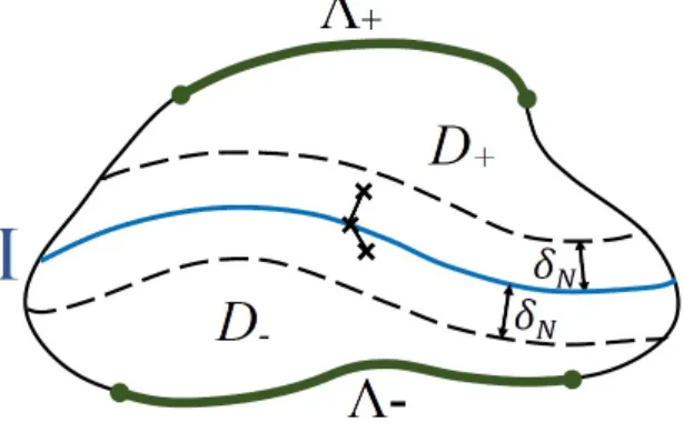
Here is a heuristic description of our new model (See figure 1): Let D± and I be as above.
Figure 1: I = Interface, Λ±= Harvest sites
There is a harvest region Λ±⊂∂D±\I that absorbs (harvests)±charges, respectively, whenever
it is being visited. LetN be the (common) initial number of particles in each ofD+andD−. For
simplicity, we assume here that each particle inD±performs a Brownian motion with drift in the
interior of D±. These random motions model the transport of positive (respectively, negative)
charges under an electric potential. When a particle hits the boundary, it is absorbed (harvested) on Λ±, and is instantaneously reflected on∂D±\Λ±along the inward normal direction ofD±. In
other words, we assume that each particle inD± performs a reflected Brownian motions (RBM)
with drift inD± that is killed upon hitting Λ±. In addition, a pair of particles of opposite signs
has a chance of being annihilated with each other when they are near I. Actually, when two particles of different types come within a small distanceδN (which must occur near the interface I), they disappear with intensity λ
N δNd+1. Here λ >0 is a given parameter modeling the rate of annihilation.
The choice of the scaling λ
particles in D+ near I, and each of them is near to N δdN number of particles in D−). With the above choice of per-pair annihilation intensity, the expected number of pairs killed withint
units of time is about (N2δdN+1) ( λ
N δdN+1t) = λN t when t > 0 is small. This implies that a non trivial proportion of particle is annihilated during [0, t] and accounts for the boundary term in the hydrodynamic limit.
1.1 Main result and applications We consider the normalized empirical measures
XN,t +(dx) := 1
N
X
α:α∼t 1X+
α(t)(dx) and X
N,−
t (dy) := 1
N
X
β:β∼t 1X−
β(t)(dy).
Here1y(dx) stands for the Dirac measure concentrated at the pointy, whileα∼t(resp. β ∼t) denotes the condition that particle X+
α (resp. X
−
β) is alive at time t.
Our main result (Theorem 5.2) implies the following: Suppose each particle in D± is a
RBM with gradient drift 12∇(logρ±), where ρ± is a strictly positive function on D±.
Sup-pose δN tends to zero and lim infN→∞N δdN ∈ (0,∞]. If (XN,0 +,XN,0 −) converges in
distribu-tion, then the random measures (XN,t +,XN,t −) converge in distribution to a deterministic limit (u+(t, x)ρ+(x)dx, u−(t, y)ρ−(y)dy) for any t >0, where (u+, u−) is the unique solution of the
coupled heat equations
∂u+
∂t =
1
2∆u++ 1
2∇(logρ+)· ∇u+ on (0,∞)×D+
u+= 0 on (0,∞)×Λ+
∂u+
∂~n+
= λ
ρ+
u+u−1{I} on (0,∞)×∂D+\Λ+
(1.1)
and
∂u−
∂t =
1
2∆u−+ 1
2∇(logρ−)· ∇u− on (0,∞)×D−
u−= 0 on (0,∞)×Λ−
∂u−
∂~n−
= λ
ρ−
u+u−1{I} on (0,∞)×∂D−\Λ−,
(1.2)
wheren~±is the inward unit normal vector field on∂D± ofD±and1{I}is the indicator function
on I. Note that ρ±= 1 corresponds to the particular case when there is no drift.
Remark 1.1. Generalizations and Applications: Actually, Theorem 5.2 is general enough to deal with any general symmetric reflected diffusions and covers the case when the constant λ
is replaced by any continuous function λ(x) on I. It is routine to generalize to any continuous time-dependent function λ(t, x) and the details are left to the readers. Moreover, it is likely that a further generalization to tackle multiple deletion of particles near the interface (similar to that in [17]) can be done in an analogous way. As an immediate application of Theorem 5.2, we obtain an analytic formula for the asymptotic mass of positive charges harvested during the time interval [0, T], which is
1−
Z
D+
u+(T, x)ρ+(x)dx−λ
Z T
0
Z
I
Remark 1.2. The condition lim infN→∞N δNd ∈(0,∞] is an upper bound for the rate at which
the annihilations distance δN tends to 0. Such kind of condition is necessary by the following reason: The dimension of I is d+ 1 lower than that of D+×D−. So we can choose δN small enough so that particles of different types cannot ‘see’ each other in the limitN → ∞, resulting a decoupled linear system of PDEs with Dirichlet boundary condition on Λ± and Neumann
boundary condition on∂D±\Λ±. See Example 5.3 for a rigorous statement and proof.
1.2 Key ideas
Theorem 3.2.39 of [22] from geometric theory asserts that
lim δ→0
H2d(Iδ) cd+1δd+1
=Hd−1(I), (1.3)
where Iδ :={(x, y) ∈D+×D− : |x−z|2+|y−z|2 < δ2 for somez ∈I}, cd+1 is the volume
of the unit ball in Rd+1, and Hm is the m-dimensional Hausdorff measure. In Lemma 7.2, we strengthen it to
lim δ→0
1
cd+1δd+1
Z
Iδ
f(x, y)dxdy =
Z
I
f(z, z)dHd−1(z) (1.4)
uniformly inf from any equi-continuous family in C(D+×D−). Property (1.4) leads us to the
following key observation that
lim δ→0Nlim→∞
1
cd+1δd+1E
Z T
0
XN,s +⊗XN,s −(Iδ)ds= lim N→∞δlim→0
1
cd+1δd+1E
Z T
0
XN,s +⊗XN,s −(Iδ)ds.
This interchange of limit in turn allows us to characterize the mean of any subsequential limit of (XN,+,XN,−) by comparing the integral equations (4.1) satisfied by the hydrodynamic limit with its stochastic counterpart (7.6) . Using a similar argument, we can identify the second moment of any subsequential limit, and hence characterize any subsequential limit of (XN,+,XN,−). We point out here that c 1
d+1δd+1 Rt
0X
N,+
s ⊗XN,s −(Iδ)ds quantifies the amount of interaction among the two types of particles, and is related (but different from) thecollision local time introduced in [20]. The direct approach developed in this paper to establish the hydrodynamic limit avoids going through the delicate BBGKY hierarchy as was done in [9].
1.3 Literature
Interacting diffusion systems have been studied by many authors and they continue to be the subject of active research. See [30] and [32] for such a system on a circle whose hydrodynamic limit is established using the entropy method. We also mention [16] for a recent large deviation result for a system of diffusions in R interacting through their ranks. This large deviation principle implies convergence of the system to the hydrodynamic limit. However, the methods in these papers do not seem to work (at least not in a direct way) for our annihilating diffusion model due to the singular interaction on the interface.
authors in both the discrete setting (particles perform random walks) and the continuous setting (particles perform continuous diffusions). For instance, for the caseR(u) is a polynomial inu, these systems were studied in [17, 18, 28, 29] on a cube with Neumann boundary conditions, and in [3, 4] on a periodic lattice. See also [7] for a survey of a class of discrete (lattice) models called the Polynomial Model which contains the Schl¨ogl’s model. Recently, perturbations of the voter models which contain theLotka-Volterra systems are considered in [13]. The authors showed that the hydrodynamic limits are R-D equations and established general conditions for the existence of non-trivial stationary measures and for extinction of the particles. Another stochastic particle systems which are related to our annihilation-diffusion model is the Fleming-Viot type systems ([5, 6, 24]). In [6], Burdzy and Quastel studied an annihilating-branching system of two families of random walks on a domain. In their model, when a pair of parti-cles of different types meet, they annihilate each other and they are immediately reborn at a site chosen randomly from the remaining particles of the same type. So the total number of particles of each type remains constant over the time, and thus this Fleming-Viot type system is different from the annihilating random walk model of [9]. The hydrodynamic limit of the model in [6] is described by a linear heat equation with zero average temperature. An elegant result obtained by P. Dittrich [17] is on a system of reflected Brownian motion on the unit interval [0,1] with multiple deletion of particles. More precisely, any k-tuples (2 ≤ k ≤ n) of particles with distances between them of order ε, say (xi1,· · ·, xik), disappear with intensity
ck(k−1)!εk−1
R
[0,1]p(ε2, xi1, y)· · ·p(ε2, xik, y)dy, where ck > 0 are constants and p(t, x, y) is
the transition density of the reflected Brownian motion on [0,1]. The hydrodynamic limit is a R-D equation with reaction term R(u) = −Pn
k=2ckuk and Neumann boundary condition. In contrast to [17], our model has two types of particles instead of one. Moreover, the interaction of our model is singular near the boundary and gives rise to a boundary integral term in the hydrodynamic limit.
The rest of the paper is organized as follows. Preliminary materials on setup, reflecting diffu-sions, and notations are given in Section 2. A rigorous description of the interacting stochastic particle system we are going to study in this paper is presented in Section 3. In section 4, we give an existence and uniqueness result of solution of a coupled heat equation with non-linear boundary condition, analogous to [9, Proposition 2.19]. The full statement of our main result (Theorem 5.2) of this paper is given in section 5. Section 6 is devoted to the proof of Theorem 5.2. The proof of a key proposition that identifies the first and second moments of subsequential limits of empirical distributions is given in Section 7.
2
Preliminaries
2.1 Reflected diffusions killed upon hitting a closed set Λ ⊂D
LetD⊂Rdbe a bounded Lipschitz domain, and
W1,2(D) ={f ∈L2(D;dx) :∇f ∈L2(D;dx)}.
Consider the bilinear form onW1,2(D) defined by
E(f, g) := 1 2
Z
D
where ρ ∈W1,2(D) is a positive function on D which is bounded away from zero and infinity, a = (aij) is a symmetric bounded uniformly elliptic d×d matrix-valued function such that
aij ∈W1,2(D) for each i, j. SinceDis Lipschitz boundary, (E, W1,2(D)) is a regular symmetric Dirichlet form onL2(D;ρ(x)dx) and hence has a unique (in law) associatedρ-symmetric strong Markov processX (cf. [8]).
Definition 2.1. Let (a, ρ) and X be as in the preceding paragraph. We call X an (a, ρ) -reflected diffusion. A special but important case is when a is the identity matrix, in which
X is called a reflected Brownian motion with drift 12∇(logρ). If in addition ρ = 1, then X is called a reflected Brownian motion (RBM).
Denote by~nthe unit inward normal vector ofDon ∂D. The Skorokhod representation ofX
tells us (see [8]) thatX behaves like a diffusion process associated to the elliptic operator
A:= 1
2ρ∇ ·(ρa∇) (2.1)
in the interior of D, and is instantaneously reflected at the boundary in the inward conormal direction ~ν := a~n. It is well known (cf. [2, 25] and the references therein) that X has a transition density p(t, x, y) with respect to the symmetrizing measure ρ(x)dx (i.e., Px(Xt ∈ dy) = p(t, x, y)ρ(y)dy and p(t, x, y) =p(t, y, x)), that p is locally H¨older continuous and hence
p ∈ C((0,∞)×D×D), and that we have the followings: for any T > 0, there are constants
c1 ≥1 andc2 ≥1 such that
1
c1td/2
exp
−
c2|y−x|2
t
≤p(t, x, y)≤ c1 td/2 exp
−|
y−x|2
c2t
(2.2)
for every (t, x, y)∈(0, T]×D×D. Using (2.2) and the Lipschitz assumption for the boundary, we can check that
sup x∈D
sup
0<δ≤δ0
1
δ
Z
Dδ
p(t, x, y)dy ≤ √C1
t+C2 fort∈(0, T] and (2.3)
sup x∈D
Z
∂D
p(t, x, y)σ(dy) ≤ √C1
t+C2 fort∈(0, T], (2.4)
whereC1, C2, δ0>0 are constants which depends only ond,T, the Lipschitz characteristics of
D, the ellipticity ofaand the lower and upper bound ofρ. HereDδ:={x∈D: dist(x, ∂D)< δ}. In fact (2.4) follows from (2.3) via Lemma 7.1.
Now we consider an (a, ρ)-reflected diffusion killed upon hitting a closed subset Λ of D. In particular, Λ can be subset of∂D (this is the case for Λ± in figure 1). Define
Xt(Λ):=
(
Xt, t < TΛ
∂, t≥TΛ,
(2.5)
where ∂ is a cemetery point and TΛ := inf{t >0 : Xt∈Λ} is the first hitting time of X on Λ. Since D\Λ is open in D, Theorem A.2.10 of [23] asserts that X(Λ) is a Hunt process on (D\Λ)∪∂ with transition function PtΛ(x, A) = Px(Xt ∈ A, t < TΛ). The characterization
on L2(D\Λ, ρ(x)dx). Clearly, X(Λ) has a transition density p(Λ) with respect to ρ(x)dx (i.e.
PtΛ(x, dy) =p(Λ)(t, x, y)ρ(y)dy). Note thatp(Λ)(t, x, y)≤p(t, x, y) for all x, y∈D and t >0. So far Λ is only assumed to be closed in D. We will also need the following regularity assumption.
Definition 2.2. Λ⊂Dis said to be regularwith respect toX if Px(TΛ = 0) = 1for allx∈Λ,
where TΛ:= inf{t >0 : Xt∈Λ}.
This regularity assumption implies thatp(Λ)(t, x, y) is jointly continuous inx andy up to the boundary. In particular,p(Λ)(t, x, y) is continuous forx and y in a neighborhood of I. We now gather some basic properties ofp(Λ)(t, x, y) for later use.
Proposition 2.3. LetXbe an(a, ρ)-reflected diffusion defined in Definition 2.1, andp(Λ)(t, x, y) be the transition density, with respect toρ(x)dx, ofXΛ defined in (2.5). SupposeΛ is closed and regular with respect to X. Then p(Λ)(t, x, y) ≥0 and p(Λ)(t, x, y) =p(Λ)(t, y, x) for all x, y∈D
and t >0. Moreover, p(Λ)(t, x, y) can be extended to be jointly continuous on (0,∞)×D×D. The last property implies that the semigroup {PΛ
t }t≥0 of XΛ is strongly continuous on the
Ba-nach spaceC∞(D\Λ) :={f ∈C(D) : f vanishes on Λ} equipped with the uniform norm onD.
The domain of the Feller generator of{Pt(Λ)}t≥0, denoted byDom(A(Λ)), is dense inC∞(D\Λ).
Proof Define, for all (t, x, y)∈(0,∞)×D×D,
q(Λ)(t, x, y) :=p(t, x, y)−r(t, x, y), wherer(t, x, y) :=Ex[p(t−TΛ, XTΛ, y);t≥TΛ].
Using the fact that x 7→ Px(T
Λ < t) is lower semi-continuous (cf. Proposition 1.10 in Chapter
II of [1]), it is easy to check that if Λ is closed and regular, then
lim n→∞P
xn(T
Λ< t) = 1 (2.6)
whenever t > 0 and xn ∈ D converges to a point in Λ. Recall that p(t, x, y) is symmetric in (x, y), has two-sided Gaussian estimates (2.2), and is jointly continuous on (0,∞)×D×D. Using these properties of p together with (2.6), then applying the same argument of section 4 of Chapter II in [1], we have
(a) q(Λ)(t, x, y) is a density for the transition functionXΛ.
(b) q(Λ)(t, x, y)≥0 andq(Λ)(t, x, y) =q(Λ)(t, y, x) for allx, y∈Dand t >0.
(c) q(Λ)(t, x, y) is jointly continuous on (0,∞)×D×D.
From (c), the semigroup{Pt(Λ)}ofX(Λ)is strongly continuous by a standard argument. C
∞(D\
Λ) is a Banach space since it is a closed subspace ofC(D). The Feller generator Dom(A(Λ)) of
{Pt(Λ)}is dense inC∞(D\Λ) because anyf ∈C∞(D\Λ) is the strong limit limt↓0 1t
Rt
0P (Λ)
s f ds inC∞(D\Λ), and
Rt
0P (Λ)
s f ds∈Dom(A(Λ)).
2.2 Assumptions and notations
absorption on Λ±⊂∂D±\I. If a particle is absorbed (in Λ±) rather than annihilated (nearI),
it is considered to be harvested.
The following assumptions are in force throughout this paper.
Assumption 2.4. (Geometric setting) Suppose D+ and D− are given adjacent bounded
Lip-schitz domains in Rd such that I := D+ ∩D− = ∂D+ ∩∂D− is Hd−1-rectifiable. Λ± is a
closed subset of D± \I which is regular with respect to the (a±, ρ±)-reflected diffusion X±,
whereρ±∈W(1,2)(D±)∩C(D±) is a given strictly positive function,a±= (aij±) is a symmetric,
bounded, uniformly ellipticd×dmatrix-valued function such that aij± ∈W1,2(D
±) for each i, j.
Assumption 2.5. (Parameter of annihilation) Suppose λ ∈ C+(I) is a given non-negative
continuous function on I. Let bλ∈C(D+×D−) be an arbitrary but fixed extension of λin the
sense that bλ(z, z) =λ(z) for all z∈I. (Such bλalways exists.)
Assumption 2.6. (The annihilation distance)lim infN→∞N δNd ∈(0,∞], where{δN} ⊂(0,∞) converges to 0 as N → ∞.
Assumption 2.7. (The annihilation potential) We chooseannihilation potential functions
{`δ: δ >0} ⊂C+(D+×D−) in such a way that `δ≤ c bλ
d+1δd+11Iδ on D+×D− and
lim δ→0
`δ−
b
λ cd+1δd+1
1Iδ
L2(D +×D−)
= 0 (2.7)
Assumption 2.7 is natural in view of (1.3). Intuitively, ifN is the initial number of particles, thenδN is the annihilation distance andIδN controls the frequency of interactions. As remarked in the introduction, we need to assume that the annihilation distance δN does not shrink too fast. This is formulated in Assumption 2.6.
Convention: To simplify notation, we suppress Λ± and write X± in place of XΛ± for a
(a±, ρ±)-reflected diffusions on D± killed upon hitting Λ±. We also use p±(t, x, y),Pt± andA±
to denote, respectively, the transition density w.r.t. ρ±, the semigroup associated top±(t, x, y)
and theC∞(D±\Λ±)-generator (called the Feller generator) ofX±=XΛ±. Under Assumption
2.4, X± is a Hunt (hence strong Markov) process on
D∂±:=D±\Λ±
∪ {∂±},
where∂± is the cemetery point forX± (see Proposition 2.3).
For reader’s convenience, we list other notations that we will adopt here:
B(E) Borel measurable functions onE
Bb(E) bounded Borel measurable functions onE B+(E) non-negative Borel measurable functions on E
C(E) continuous functions onE
Cb(E) bounded continuous functions onE C+(E) non-negative continuous functions onE
Cc(E) continuous functions onE with compact support D([0,∞), E) space ofcadl` `ag paths from [0,∞) to E
C∞(D\Λ) {f ∈C(D) : f vanishes on Λ}
C∞(n,m) Φ∈C(D
n
+×D
m
−) : Φ vanishes outside (D+\Λ+)n×(D−\Λ−)m ,
see Subsection 7.2
Hm m-dimensional Hausdorff measure
Iδ {(x, y)∈D+×D−: |x−z|2+|y−z|2< δ2 for somez∈I},
cd+1 the volume of the unit ball in Rd+1
`δ the annihilating potential functions in Assumption 2.7
X(tN) the configuration process defined in Subsection 3.1
SN ∪Nm=1 D∂+(m)×D∂−(m)
∪ {∂}, the state space of (X(tN))t≥0
(XN,t +,XN,t −) the normalized empirical measure defined in Subsection 3.2
EN ∪NM=1EN(M)∪ {0∗}, the state space of (XN,t +,XN,t −)t≥0
M+(E) space of finite non-negative Borel measures on E, with weak topology
M≤1(E) {µ∈M+(E) : µ(E)≤1}
M M≤1(D+\Λ+)×M≤1(D−\Λ−), see Section 5
{FX
t : t≥0} filtration induced by the process (Xt), i.e. FtX =σ(Xs, s≤t) 1x indicator function atx or the Dirac measure atx
(depending on the context)
L
−→ convergence in law of random variables (or processes) hf, µi R
f(x)µ(dx)
x∨y max{x, y} x∧y min{x, y}
3
Annihilating diffusion system
In this section, we fixN ∈Nand construct the normalized empirical measure process (XN,+,XN,−) and the configuration process X(N) for our annihilating particle system. In the construction, we will label (rather than annihilate) pairs of particles to keep track of the annihilated parti-cles. This provides acoupling of our annihilating particle system and the corresponding system without annihilation.
Let m ∈ {1,2,· · ·, N} (in fact, m can be any positive integer). Starting with m points in each ofD∂+ and D−∂, we perform the following construction:
Let{Xi± =XΛ±
i }mi=1 be (a±, ρ±)-reflected diffusions on D± killed upon hitting Λ±, starting
from the given points inD∂±. These 2m processes are constructed to be mutually independent.
In case Xi± starts at the cemetery point ∂±, we haveXi±(t) =∂±for all t≥0. Let{Rk}mk=1 be
i.i.d. exponential random variables with parameter one which are independent of{Xi+}m i=1 and
{Xi−}m j=1.
Define the first time of labeling (or annihilation) to be
τ1 := inf
t≥0 : 1 2N
Z t
0
m
X
i=1
m
X
j=1
`δN(X
+
i (s), X
−
j (s))ds≥R1
In the above, `δN(x, y) = 0 if either x = ∂
+ or y = ∂−. Hence particles absorbed at Λ ± do
not contribute to rate of labeling (or annihilation). At τ1, we label exactly one pair in {(i, j)}
according to the probability distribution given by
`δN(X
+
i (τ1−), Xj−(τ1−))
Pm
p=1
Pm
q=1`δN(X
+
p (τ1−), Xq−(τ1−))
assigned to (i, j).
Denote (i1, j1) to be the labeled pair at τ1 (think of the labeled pair as begin removed due to
annihilation of the corresponding particles).
We repeat this labeling procedure using the remaining unlabeled 2(m−1) particles. Precisely, fork= 2,3,· · ·, m, we define
τk:= inf
t≥0 : 1 2N
Z τ1+···+τk−1+t
τ1+···+τk−1
X
i /∈{i1,···,il−1}
X
j /∈{j1,···,jl−1}
`δN(X
+
i (s), X
−
j (s))ds≥Rk
.
At σk := τ1 +τ2 +· · ·+τk−1+τk, the k-th time of labeling (annihilation), we label exactly one pair (ik, jk) in {(i, j) : i /∈ {i1,· · · , ik−1}, j /∈ {j1,· · ·, jk−1} } according to the probability
distribution given by
`δN(X
+
i (σk−), Xi−(σk−))
P
i /∈{i1,···,ik−1} P
j /∈{j1,···,jk−1}`δN(X
+
i (σk−), X
−
i (σk−))
assigned to (i, j).
We will study the evolution of the unlabeled (or surviving particles, which is described in detail below.
3.1 The configuration process X(N)
We denote D∂±(m) the space of unordered m-tuples of elements in D±∂ :=
D±\Λ±
∪ {∂±}. Theconfiguration space for the particles is defined as
SN :=∪Nm=1
D+∂(m)×D−∂(m)
∪ {∂}, (3.2)
where∂ is a cemetery point (different from∂±).
We define X(tN) ∈SN to be the following unordered list of (the position of) unlabeled (sur-viving) particles at timet. That is,
X(tN) :=
{X1+(t),· · ·, Xm+(t)}, {X1−(t),· · · , Xm−(t)}
, ift∈[0, σ1=τ1);
{Xi+(t)}i /∈{i1,···,i
k−1}, {X
−
j (t)}j /∈{j1,···,jk−1}
, ift∈[σk−1, σk), fork= 2,3,· · ·, m;
∂, ift∈[σm,∞).
By definition,X(tN)∈D+∂(m−k+ 1)×D−∂(m−k+ 1) whent∈[σk−1, σk), andX(tN) =∂if and only if all particles are labeled (annihilated) at time t(in particular, none of them is absorbed at Λ±). We callX(N)= (Xt(N))t≥0 theconfiguration process.
Denote (Ω,F, ℘) the ambient probability space on which the above random objects{Xi+}m i=1,
{Xi−}m
j=1, {Ri}mi=1 and {(i1, j1),· · ·,(im, jm)} are defined. For any z∈SN, we definePz to be the conditional measure℘ · |X(0N) =z
Proposition 3.1. {X(N)} is a strong Markov processes under{
Pz : z∈SN}.
The key is to note that the choice of (ik, jk) depends only on the value of X(σNk)−, and that
τk+1 = inf{t≥0 : A (k)
t > Rk+1}, where A (k)
t = 1 2N
Z σk+t
σk X
i=1
X
j=1
`δN(X
+
i (s), X
−
j (s))ds.
Hence X(N) is obtained through a patching procedure reminiscent to that of Ikeda, Nagasawa and Watanabe [26]. The proof is standard and is left to the reader.
3.2 The normalized empirical process (XN,+,XN,−)
Next, we considerEN :=∪NM=1E (M)
N ∪ {0∗}, where
E(NM):=
1
N M
X
i=1
1xi, 1
N M
X
j=1
1yj
: xi ∈D∂+, yj ∈D∂−
and 0∗ is an abstract point isolated from ∪NM=1EN(M). We define the normalized empirical
measure(XN,+,XN,−) by
(XN,t +,XN,t −) :=UN(X(tN)), (3.3) whereUN : SN →EN is the canonical map given byUN(∂) :=0∗ and
UN : (x, y) = (x1,· · ·, xm, y1,· · · , ym)7→
1
N m
X
i=1
1xi, 1
N m
X
j=1
1yj
For comparison, we also consider the empirical measure for the independent reflected diffusions without annihilation:
(XN,+,XN,−) :=
1
N m
X
i=1
1X+ i (t),
1
N m
X
j=1
1X−
j(t)
. (3.4)
For anyµ∈EN, we definePµto be the conditional measure℘ · |(XN,0 +,X
N,−
0 ) =µ
. From Proposition 3.2, we have
Proposition 3.2. {(XN,+,XN,−)} is a strong Markov processes under{Pµ: µ∈E N}.
4
Coupled heat equation with non-linear boundary condition
Denote byC∞([0, T];D\Λ) the space of continuous functions on [0, T] taking values inC∞(D\
Λ) := {f ∈ C(D) : f vanishes on Λ}. We equip the Banach space C∞([0, T];D+ \Λ+)×
C∞([0, T];D−\Λ−) with norm k(u, v)k := kuk∞+kvk∞, where k · k∞ is the uniform norm.
Proposition 4.1. LetT >0andu±0 ∈C∞(D±\Λ±). Then there is a unique element(u+, u−)∈
C∞([0, T];D+\Λ+)×C∞([0, T];D−\Λ−) that satisfies the coupled integral equation
(
u+(t, x) =PΛ
+
t u+0(x)−12
Rt
0
R
IpΛ
+
(t−r, x, z)[λ(z)u+(r, z)u−(r, z)]dσ(z)dr
u−(t, y) =PΛ −
t u
−
0(y)− 1 2
Rt
0
R
Ip
Λ−(t−r, y, z)[λ(z)u
+(r, z)u−(r, z)]dσ(z)dr.
(4.1)
Moreover, (u+, u−) satisfies
u+(t, x) =Ex
h
u+0(XtΛ+) exp−
Z t
0
(λ·u−)(t−s, XΛ
+
s )dLI,s+
i
u−(t, y) =Ey
h
u−0(XtΛ−) exp−
Z t
0
(λ·u+)(t−s, XΛ
−
s )dLI,s−
i
,
(4.2)
where LI,± is the boundary local time of XΛ± on the interface I, i.e. the positive continuous additive functional having Revuz measure σ|I, the surface measure σ restricted to I.
It can be shown that continuous functions (u+, u−) satisfying (4.1) is weakly differentiable
and satisfies the following PDE (4.3)-(4.4) in the distributional sense.
Definition 4.2. We call the unique solution(u+, u−)∈C∞([0, T];D+\Λ+)×C∞([0, T];D−\
Λ−) of (4.1)the weak solution to the following coupled PDEs starting from (u+0, u−0):
∂u+
∂t =A
+u
+ on(0,∞)×D+
u+= 0 on(0,∞)×Λ+
∂u+
∂ ~ν+
= λ
ρ+
u+u−1{I} on(0,∞)×∂D+\Λ+
(4.3)
and
∂u−
∂t =A
−
u− on (0,∞)×D−
u−= 0 on (0,∞)×Λ−
∂u−
∂ ~ν−
= λ
ρ−
u+u−1{I} on (0,∞)×∂D−\Λ−,
(4.4)
where ν~± := a±~n± is the inward conormal vector field on ∂D±. Here 1{I} is the indicator
function ofI.
5
Main result: rigorous statement
Denote byM≤1(D±\Λ±) the space of non-negative Borel measures on D±\Λ± with mass at
most 1 and set
M:=M≤1(D+\Λ+)×M≤1(D−\Λ−),
equipped with the topology of weak convergence.
Remark 5.1. M is in fact a Polish space. Let {fn;n ≥ 1} and {gn;n ≥ 1} be sequences of continuous functions with |fn| ≤1 and |gn| ≤ 1 whose linear span are dense in C∞(D+\Λ+)
and C∞(D−\Λ−), respectively. For µ= (µ+, µ−) and ν = (ν+, ν−) in M, define
%(µ, ν) :=
∞
X
n=1
2−n
Z
D+
fn(x)(µ+−ν+)(dx)
+
Z
D−
gn(y)(µ−−ν−)(dy)
It is well known thatM is a complete separable metric space under the metric%.
Regard 1∂± as 0± and 0∗ as (0+,0−), where 0± is the zero measure on D±, respectively.
Clearly,EN ⊂Mfor allN, and the processes (XN,+,XN,−) have sample paths inD([0,∞),M), the Skorokhod space ofcadl` `ag paths in M.
We can now rigorously state our main result. In what follows, −→L denotes convergence in law.
Theorem 5.2. (Hydrodynamic Limit) Suppose that Assumptions 2.4 to 2.7 hold. If asN → ∞, (XN,0 +,XN,0 −)−→L (u0+(x)ρ+(x)dx, u−0(y)ρ−(y)dy) in M, where u0±∈C∞(D±\Λ±), then
(XN,+,XN,−)−→L (u+(t, x)ρ+(x)dx, u−(t, y)ρ−(y)dy) in D([0, T],M)
for any T > 0, where (u+, u−) is the unique weak solution of (4.3)-(4.4) with initial value
(u0 +, u0−).
As mentioned in Remark 1.2 in the introduction, an assumption on the rate at which δN tends to zero, such as Assumption 2.6, isnecessary for Theorem 5.2 to hold. Below is a counter-example.
Example 5.3. Suppose that {Xi+(t)}∞i=1 and {Xj−(t)}∞j=1 are RBMs on D+ and D−,
respec-tively, and they are all mutually independent. Note thatXi+ and Xj− never meet in the sense that
P
Xi+(t) =Xj−(t) for some t∈[0,∞) and i, j ∈ {1,2,3,· · · }= 0. (5.1)
This implies that there exists{δN}so that P∞N=1αN <∞, where
αN :=P
(Xi+(t), Xj−(t))∈IδN for somet∈[0,∞) andi, j ∈ {1,2,· · ·, N}
. (5.2)
Hence by Borel-Cantelli lemma, we know that with probability 1, there will be no annihila-tion for the particle system (which occurs only when a pair of particles are in IδN) whenN is sufficiently large. In this case, (XN,t +,XN,t −) converges to (Pt+u+0(x)dx, Pt−u−0(y)dy) in distri-bution inD([0, T],M) instead, provided that (XN,0 +,X0N,−) converges to (u+0(x)dx, u−0(y)dy) in distribution inM.
Question. We will see from Theorem 6.6 below that the tightness of (XN,t +,XN,t −) holds without Assumption 2.6. Can we characterize all limit points of (XN,t +,XN,t −) without Assumption 2.6? Is lim infN→∞N δNd ∈(0,∞] the sharpest condition for Theorem 5.2 to hold?
6
Hydrodynamic limit
Recall that Assumptions 2.4 to 2.7 are in force throughout this paper.
6.1 Martingales and tightness
6.1.1 Martingales for reflected diffusions
We will need the following collection of fundamental martingales, together with their quadratic variations, for reflected diffusions.
Lemma 6.1. SupposeXΛis an(a, ρ)-reflected diffusion in a bounded Lipschitz domainDkilled upon hittingΛ. Suppose all assumptions in Proposition 2.3 hold, and f is in the domain of the Feller generator Dom(A(Λ)). Then we have
M(t) :=f(XΛ(t))−f(XΛ(0))−
Z t
0
A(Λ)f(XΛ(s))ds (6.1)
is anFXΛ
t -martingale that is bounded on each compact time interval and has quadratic variation
Rt
0(a∇f · ∇f) (X
Λ(s))dsunder
Px for any x∈D\Λ. Moreover, if X1 and X2 are independent
copies of XΛ, and if Mi is the above M with XΛ replaced by Xi, then the cross variation hM1, M2it= 0.
Proof Forf ∈Dom(A(Λ)),M(t) defined in (6.1) is anFXΛ
t -martingale that is bounded on each compact time interval. Since D is bounded, f is clearly in the domain of the L2-generator of
XΛ. Hence it follows from the Fukushima decomposition off(XtΛ) (see [11, Theorems 4.2.6 and 4.3.11] that M(t) is a martingale additive functional of XΛ of finite energy having quadratic variationhM(t)it=R0t(a∇f· ∇f)(XΛ(s))ds. IfX1 and X2 are independent copies of XΛ, then
M1 and M2 are independent and sohM1, M2i= 0.
An immediate consequence of Lemma 6.1 is
Z t
0
PsΛ(a∇f· ∇f)(x)ds=Ex[M(t)2]≤8(kfk2+kA(Λ)fk2t2) forx∈D, (6.2)
wherekgkis the uniform norm of g onD.
6.1.2 Martingales for annihilating diffusion system
Theorem 6.2. Fix any positive integer N. Suppose F ∈ Cb(EN) is a bounded continuous function and G∈ B(EN) is a Borel measurable function onEN such that
Mt:=F(X N,+
t ,X N,−
t )−
Z t
0
G(XN,s +,XN,s −)ds
is an F(X
N,+
,XN,−)
t -martingale under Pµ for any µ∈EN. Then
Mt:=F(XN,t +,X N,−
t )−
Z t
0
(G+KF)(XN,s +,XN,s −)ds
is a Ft(XN,+,XN,−)-martingale under Pµ for any µ∈EN, where
KF(ν) :=− 1 2N
M
X
i=1
M
X
j=1
`δN(xi, yj)
F(ν) − F ν+−N−11{xi}, ν
−−N−11
{yj}
(6.3)
whenever ν =
1
N
PM
i=11{xi},
1
N
PM
j=11{yj}
Remark 6.3. (i) Theorem 6.2 indicates the infinitesimal generator of (XN,+,XN,−) onCb(EN) is given by L+K, where L is the infinitesimal generator of (XN,+,XN,−) on Cb(EN). Note thatGis merely assumed to be Borel measurable, the above provides us with a broader class of martingales (such asN(φ+,φ−)
t in Corollary 6.4) than from using theCb(EN)-generator.
(ii) Theorem 6.2 can be generalized to deal with time-dependent functions Fs ∈ Cb(EN) (s≥0). See Theorem 7.6 in subsection 7.2.
Proof of Theorem 6.2. We adopt the abbreviationX:= (XN,+,XN,−) when there is no confusion. In particular, we write FX
t in place of F
(XN,+,XN,−)
t . By Markov property for X, it suffices to show that for all t≥0 and ν∈EN,
Eν
h
F(Xt)−F(X0)−
Z t
0
(G+KF)(Xs)dsi= 0. (6.4)
The idea is to spit the time interval [0, t] into pieces according to the jumping times ofF(Xs) (s∈ [0, t]) caused by annihilation (excluding the jumps caused by absorbtion at the harvest sites Λ±), then applyM in each piece and take into account the jump distributions.
Suppose ν = (ν+, ν−) = (N1 Pm i=11xi,
1
N
Pm
j=11yj) ∈ E
(m)
N . Recall that σi := τ1 +· · ·τi (i= 1,2,· · ·, m) is the time of thei-th labeling (annihilation) of particles. write
F(Xt)−F(X0) =
m
X
i=0
F(X(t∧σi+1)−)−F(Xt∧σi)
+ m
X
j=1
F(Xt∧σj)−F(X(t∧σj)−)
, (6.5)
whereσ0 := 0,σm+1:=∞ and Xs−:= limr%sXr. Hence it suffices to show that
Eν
h
F(X(t∧σi+1)−)−F(Xt∧σi)−
Z t∧σi+1
t∧σi
G(Xs)ds
i
= 0 and (6.6)
Eν
h
F(Xt∧σj)−F(X(t∧σj)−)− Z t∧σj
t∧σj−1
KF(Xs)dsi = 0 (6.7)
fori∈ {0,1,2,· · · , m} and j∈ {1,2,· · · , m}.
The left hand side of (6.6) equals
Eν
Eν
h
F(X(t∧σi+1)−)−F(Xt∧σi)−
Z t∧σi+1
t∧σi
G(Xs)ds
F
X t∧σi
i
= Eν
EXσi
h
F(X(t∧σ
i+1−σi)−)−F(X0)−
Z t∧σi+1−σi
0
G(Xs)dsi1t>σi
= Eν
EXσi
h
F(X((t−σ
i)∧τi+1)−)−F(X0)−
Z (t−σi)∧τi+1
0
G(Xs)dsi1t>σi
.
The first equality follows from the strong Markov property ofX (applied to the stopping time
σi) and the fact that the expression inside the expectation vanishes when t ≤ σi. Note that σi is regarded as a constant w.r.t. the expectation EXσi, because FσXi contains the sigma-algebra generated by σi. The second equality follows from the easy fact that (t∧σi+1)−σi = (t−σi)∧(σi+1−σi) = (t−σi)∧τi+1 on t > σi. Therefore, to establish (6.6), it is enough to show that for any η∈EN and w≥0, we have
Eη
h
F(X(w∧τ)−)−F(X0)−
Z w∧τ
0
G(Xs)ds
i
whereτ is the time of the first annihilation forXstarting fromη (i.e. τ =τ1 underPη whereτ1
is defined by (3.1)).
(6.8) obviously holds if η is the zero measure since both sides vanish. Suppose η ∈ EN(n). Observe that τ is a stopping time for ˜FX
t := σ(FtX,{Ri; 1 ≤ i ≤ n}) and that Mt is a ˜FtX -martingale underPη since{Ri} is independent ofXunderPη. Hence, by the optional sampling theorem, (6.8) is true, and so is (6.6).
Following the same arguments as above, the left hand side of (6.7) equals
Eν
EXσj−1 h
F(X(t−σj−1)∧τj)−F(X((t−σj−1)∧τj)−) +
Z (t−σj−1)∧τj
0
KF(Xs)ds
i
1t>σj−1
,
whereσj−1 is regarded as a constant w.r.t. the expectationEXσj−1. Therefore, (6.7) holds if for
any η∈EN and θ≥0, we have
Eη
h
F(Xθ∧τ)−F(X(θ∧τ)−)−
Z θ∧τ
0
KF(Xs)dsi= 0, (6.9)
whereτ is the time of the first killing forXstarting from η.
Supposeη= (N1 Pn
i=11xi,
1
N
Pn
j=11yj)∈E
(n)
N andXτ−= (
1
N
Pn
i=11X+i (τ−), 1
N
Pn
j=11Xj−(τ−)),
where {Xk± : k = 1,· · · , n} are reflected diffusions killed upon hitting Λ± in the construc-tion of X. At time τ, one pair of particles among {(Xi+,X−j) : 1 ≤ i, j ≤ n} is labeled (annihilated), where the pair (Xi+,X−j ) is chosen to be labeled (annihilated) with probability
`δN(Xi+(τ−), Xj−(τ−))
Pn p=1
Pn
q=1`δN(Xp+(τ−), Xq−(τ−)). Hence
Eη
h
F(X(θ∧τ)−)−F(Xθ∧τ)
i
(6.10)
= Eη
Eη
h
F(Xτ−)−F(Xτ)
F
X τ−
i
;τ < θ
= Eη
n
X
i=1
n
X
j=1
`δN(X
+
i (τ−), X
−
j (τ−))
Pn
p=1
Pn
q=1`δN(X
+
p (τ−), Xq−(τ−))
(6.11)
F(Xτ−) − F
Xτ−−(
1
N1Xi+(τ−),
1
N1Xj−(τ−))
;τ < θ
= Eη
−(2N)KF(Xτ−)
Pn
p=1
Pn
q=1`δN(X
+
p (τ−), Xq−(τ−))
;τ < θ
= Eη
hZ θ
0
−KF(Xs)ds
i
.
The last equality follows from the fact that
τ = inf
n
t≥0 : 1 2N
Z t
0
n
X
p=1
n
X
q=1
`δN(X
+
p (s), X
−
q (s))ds ≥R
o
,
whereRis an independent exponential random variable of parameter 1 underPη(see Proposition 2.2 of [12] for a rigorous proof). Hence (6.9) is established and the proof is complete.
The following corollary is the key to the tightness of (XN,+,XN,−). Recall that A± is the Feller generator of the diffusionX±=XΛ± on D
Corollary 6.4. Fix any positive integerN. For any φ±∈Dom(A±), we have
M(φ+,φ−)
t := hφ+,XtN,+i+hφ−,X N,−
t i
−
Z t
0
hA+φ+,XN,s +i+hA
−
φ−,XN,s −i − 1
2h`δN(φ++φ−),X
N,+
s ⊗XN,
−
s ids
is an Ft(XN,+,XN,−)-martingale under Pµ for any µ∈EN, where
hf(x, y), µ+(dx)⊗µ−(dy)i:= 1
N2
X
i
X
j
f(xi, yj) whenever µ= (N−1
X
i
1xi, N
−1X
j 1yj).
Moreover, M(φ+,φ−)
t has quadratic variation
[M(φ+,φ−)]
t = 1
N
Z t
0
ha+∇φ+· ∇φ+,XN,s +i+ha−∇φ−· ∇φ−,XN,s −i
+1
2h`δN(φ++φ−)
2,XN,+
s ⊗XN,s −i
ds (6.12)
and supt∈[0,T]Eµ[(Mt(φ+,φ−))2]≤ NC for some constant C that is independent of N and µ.
Proof From Lemma 6.1, we have the following twoF(X
N,+
,XN,−)
t -martingales forφ±∈Dom(A±):
M(tφ+,φ−) := hφ+,X
N,+
t i+hφ−,X N,−
t i −
Z t
0
hA+φ+,X
N,+
s i+hA
−
φ−,XN, −
s ids and
N(tφ+,φ−) := (hφ+,X
N,+
t i+hφ−,X
N,−
t i)2 −
Z t
0
2hφ+,X
N,+
s i+hφ−,X
N,−
s i
hA+φ+,X
N,+
s i+hA−φ−,X
N,−
s i
+1
N
ha+∇φ+· ∇φ+,X
N,+
s i+ha−∇φ−· ∇φ−,X N,−
s i
ds.
Note that F1(µ) = F1(µ+, µ−) := hφ+, µ+i +hφ−, µ−i is a function in C(EN), with the convention thatφ±(∂±) := 0 andF1(0∗) := 0. A direct calculations shows that
KF1(µ) =
−1
2 h`δN(φ++φ−), µ
+⊗µ−i
Therefore, by Theorem 6.2,M(φ+,φ−)
t is anF
(XN,+,XN,−)
t -martingale. Similarly,F2(µ) := (hφ+, µ+i+
hφ−, µ−i)2 ∈C(EN) and
KF2(µ) =− hφ+, µ+i+hφ−, µ−i
h`δN(φ++φ−), µ
+⊗µ−i+ 1
2Nh`δN(φ++φ−)
2, µ+⊗µ−i.
Hence Theorem 6.2 asserts that
N(φ+,φ−)
t :=
hφ+,XN,t +i+hφ−,X N,−
t i
2
−
Z t
0
2
hφ+,XN,s +i+hφ−,XN,s −i
hA+φ+,XN,s +i+hA
−
φ−,XN,s −i
+1
N
ha+∇φ+· ∇φ+,XN,s +i+ha−∇φ−· ∇φ−,XN,
−
s i
−(hφ+,XN,s +i+hφ−,XsN,−i)h`δN(φ++φ−),X
N,+
s ⊗XN,
−
s i
+ 1
2Nh`δN(φ++φ−)
2,XN,+
s ⊗XN,s −ids
is anFt(XN,+,XN,−)-martingale. Since
M(φ+,φ−)
t
2
−N(φ+,φ−)
t is equal to the right hand side of (6.12), which is a continuous process of finite variation, it has to be [M(φ+,φ−)]
t. This proves (6.12). Therefore,
Eµ[(Mt(φ+,φ−))2] =Eµ
h
[M(φ+,φ−)]
t
i
≤ 1 N
Z t
0
hPs+ a+∇φ+· ∇φ+
,XN,0 +ids+
Z t
0
hPs− a−∇φ−· ∇φ−,XN,0 −ids
+1
2k(φ++φ−)
2k
Z t
0
h`δN,X
N,+
s ⊗XN,s −i
ds
≤ 1 N
8 kφ+k2+kA+φ+k2t2
+ 8 kφ−k2+kA−φ−k2t2
+1
2k(φ++φ−)
2k
Z t
0
h`δN,X
N,+
s ⊗XN,
−
s i
ds,
where we have used (6.2) in the last inequality. Finally, we show that
sup µ∈EN
Z t
0
Eµ[h`δN,X
N,+
s ⊗XN,s −i]≤1. (6.13)
Let ( ˜XN,+,X˜N,−) be the normalized empirical measure corresponding to the case Λ± being
empty sets. By applying the martingale M(φ+,φ−)
t to the case Λ± being empty sets and φ± = 1 (now 1 is in the domain of the Feller generator), we have
Z t
0
E[h`δN,X˜
N,+
s ⊗X˜N,
−
s i]ds=
h1,X˜N,0 +i −E[h1,X˜N,t +i]
≤1.
We then obtain (6.13) by a coupling of (XN,+,XN,−) and ( ˜XN,+,X˜N,−). The idea is that ( ˜XN,+,X˜N,−) dominates (XN,+,XN,−). This coupling can be constructed by labeling (rather than killing) particles which hit Λ±, using the same method of subsection 3.1. Hence we obtain
the desired bound forEµ[(Mt(φ+,φ−))2].
6.1.3 Tightness
The proof of tightness for (XN,+,XN,−) is non-trivial because E
h
h`δN,X
N,+
s ⊗XN,s −i2
i
blows
up nears= 0 in such a way that limN→∞R0tE
h
h`δN,X
N,+
s ⊗XN,s −i2
i
ds=∞. To deal with this singularity at s = 0, we will use the following lemma whose proof is based on the Prohorov’s theorem. We omit the proof here since it is simple. A proof can be found in [21].
Lemma 6.5. Let {YN} be a sequence of real-valued processes such that t 7→
Rt
0YN(r)dr is
(i) There exists q >1 such that limN→∞E[RhT |YN(r)|qdr]<∞ for any h >0,
(ii) limα&0limN→∞P(R0α |YN(r)|dr > ε0) = 0 for anyε0 >0.
Then{Rt
0 YN(r)dr}N∈N is tight in C([0, T],R).
Here is our tightness result for (XN,+,XN,−). Note that it does not require Assumption 2.6.
Theorem 6.6. (Tightness) Suppose{δN}tends to 0. Then{(XN,+,XN,−)}is tight inD([0, T],M) and any of subsequential limits is carried on CM[0, T]. Moreover, {JN} is tight in C([0, T]), where JN(t) :=
Rt
0h`δN,X
N,+
s ⊗XN,s −ids.
Proof Recall from Remark 5.1 thatM is a complete separable metric space. Since Dom(A±)
is dense in C∞(D±\Λ±), we only need to check a ”weak tightness criteria” (cf. Proposition
1.7 of [27]), i.e. it suffices to check that {(hφ+,XN,+i,hφ−,XN,−i)}N is tight in D([0, T],R2) for any φ± ∈ Dom(A±). By Prohorov’s theorem (see Theorem 1.3 and Remark 1.4 of [27]),
{(hφ+,XN,+i,hφ−,XN,−i)}N is tight inD([0, T],R2) if the following two properties (a) and (b) hold:
(a) For allt∈[0, T] andε0 >0, there exists a compact set K(t, ε0)⊂R2 such that
sup N P
(hφ+,XN,t +i,hφ−,X N,−
t i)∈/K(t, ε0)
< ε0.
(b) For allε0 >0,
lim
γ→0Nlim→∞P
sup
|t−s|<γ
0≤s,t≤T
hφ+,XN,t +i,hφ−,XN,t −i
−hφ+,XN,s +i,h φ−, XsN,−i
R2
> ε0
= 0.
Property (a) is true since we can always takeK = [−kφ+k∞,kφ+k∞]×[−kφ−k∞,kφ−k∞]. To
verify property (b), we only need to focus on XN,+. Note that (writing φ=φ+ for simplicity)
by Corollary 6.4, we have
hφ,XN,t +i − hφ,XN,s +i=
Z t
s
hA+φ, XN,r +idr−1 2
Z t
s
h`δNφ, X
N,+
r ⊗XN,
−
r idr+ (MN(t)−MN(s)), (6.14) whereMN(t) is a martingale. So we only need to verify (b) withhφ,XN,t +i − hφ,X
N,+
s i replaced by each of the three terms on the right hand side of (6.14).
The first term of (6.14) is obvious sincehA+φ, XN,+
r i ≤ kA+φk. For the third term of (6.14), recall that limN→∞EMN(t)2
= 0 by Corollary 6.4. Hence, by applying Chebyshev’s inequality and then Doob’s maximal inequality, we see that (b) is satisfied by the third term of (6.14).
For the second term of (6.14), we show that
lim
γ→0Nlim→∞P
sup
|t−s|<γ
0≤s,t≤T
Z t
s
h`δN,X
N,+
r ⊗XN,r −idr > ε0
Observe that, sinceh`δN,X
N,+
r ⊗XN,r −i is non-negative, it suffices to prove (6.15) for the domi-nating case where Λ± are empty. We now prove this together with the tightness of{JN}at one stroke by applying Lemma 6.5 to the special case q= 2 and YN(r) =h`δN,X
N,+
r ⊗XN,r −i. Using the Gaussian upper bound (2.2) for the heat kernel of the reflected diffusions, we have
lim N→∞
Z T
h
E[h`δN,X
N,+
s ⊗X N,−
s i
2
]ds≤C(d, D+, D−)kρ+k kρ−k
Z T
h
s−2dds <∞.
The hypothesis (i) of Lemma 6.5 is therefore satisfied, since (XN,+,XN,−) dominates (XN,+,XN,−). It remains to verify hypothesis (ii) of Lemma 6.5, that is, to prove that for any ε0 > 0,
limα→0limN→∞P(Jn(α)> ε0) = 0. By Corollary 6.4 again, for any φ∈Dom(A+), we have
1 2
Z t
0
h`δNφ,X
N,+
s ⊗XN,
−
s ids=hφ,X N,+
0 i − hφ,X
N,+
t i+
Z t
0
hA+φ,XN,s +ids+MN(t), (6.16)
where MN(t) is a martingale and limN→∞E
h
(MN(t))2
i
= 0 for all t > 0. Note that the left
hand side of (6.16) is comparable to JN(t) whenever we pick φ ∈ Dom(A+) in such a way that `δNφ≈ `δN. The idea is to pick φ ≈1(D+)r, then let r → 0 to bound JN(t) from above. Here 1(D+)r is the set of points in D+ whose distance from the boundary is less than r. More specifically, for anyr >0, letψr∈C(D+) be such thatψr= 1 on (D+)r,ψr= 0 onD+\(D+)2r and 0≤ψ≤1. Letφr∈Dom(A+)∩C+(D+) be such that kφr−ψrk∞=o(r). Suchφr exists sinceDom(A+) is dense inC(D
+). Then (6.16) implies
0 ≤ JN(α)
≤
Z α
0
h`δN −`δNφr,X
N,+
s ⊗XN,s −ids
+hφr,X
N,+
0 i − hφr,X
N,+
α i+kA+φrkα+|MN(α)|
≤ o(r)JN(α) +hφr,XN,0 +i+kA+φrkα+|MN(α)| whenever r >2δN.
This is because whenr >2δN,φr(x) is close to 1 on (D+)δN. Hence we have, for r >2δN,
(1−o(r))JN(α)≤ hφr,X0N,+i+kA+φrkα+|MN(α)|.
From this, we have
lim
α→0Nlim→∞P(JN(α)>3ε0)≤Nlim→∞P
hφr,XN,0 +i> ε0(1−o(r))
.
Note that 0≤φr≤1(D+)2r+o(r). So forr >0 small enough,
P
hφr,XN,0 +i> ε0(1−o(r))
≤P(h1(D+)2r,XN,0 +i> ε0/2).
Moreover, sinceXN,0 +−→L u+0(x)dxwithu+0 ∈C(D), we have
lim
r→0Nlim→∞P(h1(D+)2r,X
N,+
0 i> ε0/2) = 0.
6.2 Identifying subsequential limits
Recall that we have already established tightness of {(XN,+,XN,−);N ≥ 1} in Theorem 6.6. Hence any subsequence has a further subsequence which converges in distribution inD([0, T],M). LetP∞be the law of an arbitrary subsequential limit (X∞,+,X∞,−). ThenP∞((X∞,+,X∞,−)∈ C([0,∞),M)) = 1 by Theorem 6.6. Our goal is to show that
(X∞,+,X∞,−) = (u+(t, x)ρ+(x)dx, u−(t, y)ρ−(y)dy) P∞−a.s.
An immediate question is whetherX∞,+ and X∞,− have densities with respect to the Lebesque measure. For this, we can compare (XN,+,XN,−) with (XN,+,XN,−) to get an affirmative an-swer. The construction in subsection 3.1 provides a natural coupling between {(XN,+,XN,−)} and {(XN,+,XN,−)}. We summarize some preliminary information about (X∞,+,X∞,−) in the following lemma. Its proof can be found in [21].
Lemma 6.7.
P∞
hX∞t ,+, φ+iρ+ ≤ hPt+u+0, φ+iρ+ and hX∞t ,−, φ−iρ−≤ hPt−u
−
0, φ−iρ−
for t≥0 and φ±∈C∞(D±\Λ±)
= 1.
In particular, bothX∞t ,+andX∞t ,−are absolutely continuous with respect to the Lebesque measure for t ≥ 0. Moreover, (X∞t ,+,X∞t ,−) = (v+(t, x)ρ+(x)dx, v−(t, y)ρ−(y)dy) for some v±(t) ∈
Bb(D±) with v+(t, x)≤Pt+u+0(x) and v−(t, y)≤P
−
t u
−
0(y) for a.e. (x, y)∈D+×D−.
The characterization (X∞,+,X∞,−) will be accomplished by the following result of
“mean-variance analysis”:
Proposition 6.8. For all φ±∈C∞(D±\Λ±) and t≥0, we have
E∞[hv±(t), φ±iρ±] = hu±(t), φ±iρ±, (6.17)
E∞[hv±(t), φ±i2ρ±] = hu±(t), φ±i2ρ±. (6.18)
where v± is the density of X∞,±, w.r.t. ρ±(x)dx, stated in Lemma 6.7.
We postpone the proof of Proposition 6.8 to Section 7, and proceed to present the proof of Theorem 5.2.
6.3 Proof of Theorem 5.2
Proof Tightness of {(XN,+,XN,−)} was proved in Theorem 6.6. It remains to identify any subsequential limit. We conclude from (6.17) and (6.18) that
hX∞t ,+, φ+i=hu+(t), φ+iρ+ and hX
∞,−
t , φ−i=hu−(t), φ−iρ− P ∞-a.s.
for any fixed t > 0 and φ± ∈ C∞(D±\Λ±). Recall that (X∞,+,X∞,−) ∈ C([0,∞),M) by
Theorem 6.6 and that C∞(D± \ Λ±) is separable. Hence through rational numbers and a
countable dense subsets ofC∞(D±\Λ±) to strengthen the previous statement to
P∞
(X∞t ,+,Xt∞,−) = (u+(t, x)ρ+(x)dx, u−(t, y)ρ−(y)dy) ∈M for everyt≥0
= 1.
7
Characterization of the mean and the variance
The goal of this last section is to prove Proposition 6.8. We first strengthen a result from Geometric Measure Theory .
7.1 Minkowski content for {(z, z) : z ∈I}
We first look at a single domain and prove a related result.
Lemma 7.1. Let D ⊂Rd be a bounded Lipschitz domain. If F ⊂C(D) is an equi-continuous and uniformly bounded family of functions on D, then
lim ε→0fsup∈F
1 ε Z Dε
f(x)dx−
Z
∂D
f(x)σ(dx)
= 0.
Proof The result holds trivially when d = 1, by the uniform continuity of f. We will only consider d≥ 2. The idea is to cut ∂D into small pieces so that f is almost constant in each piece, and then apply (1.3) in each piece.
Fix η > 0. There exists δ > 0 such that |f(x)−f(y)| < η whenever |x−y| ≤ δ. Since D
is bounded and Lipschitz (or by a more general result by G. David in [14] or [15, Section 2]), we can reduce to local coordinates to obtain a partition{Qi}Ni=1 of ∂D in such a way that for
any i, Qi is the Lipschitz image of a bounded subset of Rd−1 (hence it is (Hd−1)-rectifiable), diam(Qi) ≤ δ and ∂Qi is (Hd−2)-rectifiable. Here ∂Qi is the boundary of Qi with respect to the topology induced by∂D.
Let (Qi)ε := {x ∈ D : dist(x, Qi) < ε} and (∂Qi)ε := {x ∈ D : dist(x, ∂Qi) < ε}. Since {(Qi)ε\(∂Qi)ε}Ni=1 are disjoint and∪Ni=1(Qi)ε\(∂Qi)ε ⊂ Dε ⊂ ∪Ni=1(Qi)ε, we have
N X i=1 Z
(Qi)ε
f dx−
Z Dε f dx ≤ N X i=1 Z
(∂Qi)ε
|f|dx. (7.1)
Therefore, we have
1 ε Z Dε
f dx−
Z ∂D f dσ ≤ 1 ε Z Dε
f dx− 1 ε
N
X
i=1
Z
(Qi)ε
f dx + 1 ε N X i=1 Z
(Qi)ε
f dx−
Z ∂D f dσ ≤ 1 ε N X i=1 Z
(∂Qi)ε
|f|dx+ N X i=1 1 ε Z
(Qi)ε
f dx−
Z
Qi
f dσ
by (7.1)
≤ N
X
i=1
kfk∞
|(∂Qi)ε|
ε + 1 ε Z
(Qi)ε
f−f(ξi)dx
+|f(ξi)|
|(Qi)ε|
ε −σ(Qi)
+ Z Qi
f−f(ξi)dσ
≤ η N X i=1 |
(Qi)ε|
ε +σ(Qi)
+kfk∞
N
X
i=1
|
(∂Qi)ε|
ε +
|(Qi)ε|
ε −σ(Qi)
Since ∂Qi and (Qi)ε are (Hd−2)-rectifiable and (Hd−1)-rectifiable, respectively, [22, Theorem 3.2.39] tells us that
lim ε→0
|(∂Qi)ε| c2ε2
=Hd−2(∂Qi) and lim ε→0
|(Qi)ε| ε =H
d−1(Q
i),
wherecm :=|{x∈Rm : |x|<1}|. Thus,
lim ε→0
1
ε
Z
Dε
f dx−
Z
∂D f dσ
≤2η
X
i
σ(Qi) = 2σ(∂D)η.
Sinceη >0 is arbitrary and the above estimate is uniform overf ∈ F, we get the desired result.
Now we prove an analogous result for the interfaceI.
Lemma 7.2. Under our geometric setting in Assumption 2.4, if F ⊂C(D+×D−) is an
equi-continuous and uniformly bounded family of functions onD+×D−, then
lim δ→0 supf∈F
(cd+1δ
d+1)−1
Z
Iδ
f(x, y)dx dy−
Z
I
f(z, z)dσ(z)
= 0.
Proof By the same argument as in the proof of Lemma 7.1, we can construct a nice partition {Qi}Ni=1 ofI and apply [22, Theorem 3.2.39 (p. 275)]. The only essential difference is that now
we require∂Qi\∂I to be (Hd−2)−rectifiable, where∂I is the boundary ofI with respect to the topology induced by ∂D+, or equivalently by ∂D−. Moreover, instead of (7.1), we now have
N
X
i=1
Z
(Qi)δ
f dxdy−
Z
Iδ
f dxdy
≤
N
X
i=1
Z
(∂Qi\∂I)δ
|f|dxdy. (7.2)
Note that we do not need any assumption on∂I.
Corollary 7.3. SupposeF ⊂C(D+×D−)is a family of equi-continuous and uniformly bounded
functions onD+×D−. Then
lim ε→0 fsup∈F
Z
D+ Z
D−
`ε(x, y)f(x, y)dxdy−
Z
I
f(z, z)σ(dz)
= 0.
Remark 7.4. Following the same proof as above, clearly we can strengthen Lemma 7.2 and Corollary 7.3 by only requiring F to be equi-continuous and uniformly bounded on a neigh-borhood of the interface I. We can also generalize Lemma 7.1 to deal with R
Jf(x)dσ(x) for any closed Hd−1-rectifiable subset of J of ∂D, and by requiring F to be equi-continuous and
uniformly bounded on a neighborhood ofJ.
7.2 Martingales for space-time processes
Lemma 7.5. SupposeXΛis an(a, ρ)-reflected diffusion in a bounded Lipschitz domainDkilled upon hitting a closed subsetΛ of ∂D that is regular with respect to X. Then for any T >0 and bounded measurable function φ onD\Λ, we have
PTΛ−sφ(XsΛ) is a FXΛ
s -martingale for s∈[0, T], (7.3)
underPxfor anyx∈D\Λ. Moreover, its quadratic variation isR0sa∇PTΛ−rφ·∇PTΛ−rφ(XΛ(r))dr.
Proof (7.3) follows from the Markov property ofXΛ. Denote byL(Λ)theL2-generator ofX(Λ).
Then for every t ∈ [0, T), PTΛ−sφ ∈ Dom(L(Λ)). It follows from the spectral representation of
L(Λ) that
∂PTΛ−sφ ∂s
L2 =k − L
(Λ)PΛ
T−sφkL2 ≤
kφkL2
T−s.
Thus (s, x) 7→ PTΛ−sφ(x) for s ∈ [0, T) and x ∈ D\Λ is in the domain of the Dirichlet form for the space-time process (s, Xs(Λ)). By an application of the Fukushima decomposition in the context of time-dependent Dirichlet forms, one concludes that the quadratic variation of the martingale s7→PΛ
T−sφ(XsΛ) is
Rs
0 a∇PTΛ−rφ· ∇PTΛ−rφ(XΛ(r))dr; see [31, Example 6.5.6]. As mentioned in Remark 6.3, a time-dependent version of Theorem 6.2 is valid. We now state it precisely. A proof can be obtained by following the same argument in the proof of Theorem 6.2, but now to the time dependent process (t, (XN,t +,XN,t −)). The detail is left to the reader.
Theorem 7.6. Let T >0, andfs∈Cb(EN) and gs∈ B(EN) for s∈[0, T]. Suppose
Ms:=fs(X N,+
s ,X N,−
s )−
Z s
0
gr(X N,+
r ,X N,−
r )dr
is a F(X
N,+
,XN,−)
s -martingale for s∈[0, T], underPµ for any µ∈EN. Then
Ms:=fs(XsN,+,XN,s −)−
Z s
0
(gr+Kfr)(XrN,+,XN,r −)dr
is a Fr(XN,+,XN,−)-martingale for s∈[0, T], under Pµ for any µ∈EN, where the operator K is given by (6.3).
Consider X(n,m) := (X1+,· · ·, X+
n, X
−
1,· · · , Xm−) ∈(D+∂)n×(D∂−)m, which consists of
inde-pendent copies ofX±’s. The transition density ofX(n,m) w.r.t. ρ(n,m) isp(n,m), where
p(n,m)(t,(~x, ~y),(x~0, ~y0)) := n
Y
i=1
p+(t, xi, x0i) m
Y
j=1
p−(t, yj, yj0)
ρ(n,m)(~x, ~y) :=
n
Y
i=1
ρ+(xi) m
Y
j=1
ρ−(yj).
The semigroup ofX(n,m), denoted by P (n,m)
t , is strongly continuous on
C∞(n,m):=
Φ∈C(Dn+×Dm−) : Φ vanishes outside (D+\Λ+)n×(D−\Λ−)m (7.4)
Corollary 7.7. Let n and m be any non-negative integers, T >0 be any positive number and Φ∈C∞(n,m). Consider the functionf : [0, T]×EN →Rdefined as follows: f(s,0∗) := 0and for
an arbitrary element µ∈ EN \ {0∗}, we can write µ= (N1 Pi∈A+1xi,
1
N
P
j∈A−1yj) for some index sets A+ and A−, then
f(s, µ) := X i1,···,in distinct
X
j1,···,jm distinct
PT(n,m−s)Φ(xi1,· · ·, xin, yj1,· · ·, yjm),
where the first summation is on the collection of all n-tuples (i1,· · · , in) chosen from distinct elements of A+, the second summation is on the collection of all m-tuples (j1,· · · , jm) chosen from distinct elements of A−. Then we have
f s, (XN,s +,XN,s −)
−
Z s
0
Kf(r, ·)(XN,r +,XN,r −)dr
is a Fs(XN,+,XN,−)-martingale for s∈[0, T], underPν, for anyν ∈EN.
Proof Clearly, f(s,·) ∈ Cb(EN) for s ∈ [0, T]. By Lemma 7.5, we have f(s,Xs) is a FsX -martingale for s∈[0, T] for all T ≥0. Hence we can take gr to be constant zero and fr to be f(r,·) in Theorem 7.6 to finish the proof.
As an immediate consequence, we obtain the Dynkin’s formula for our system: For 0≤t≤T, we have
E
h
f T,(XN,T +,XN,T −)−f t,(XN,t +,XN,t −)−
Z T
t
Kf(r, ·)(XN,r +,XN,r −)dr
i
= 0 (7.5)
Corollary 7.7 is the key to obtain the system of equations satisfied by the correlation functions of the particles in the annihilating diffusion system. This system of equations, usually called BBGKY hierarchy, will be formulated in the forthcoming paper [10]. The specific integral equations that we need to identify subsequential limits of {(XN,+,XN,−)} are stated in the following lemmas. These equations are a part of the BBGKY hierarchy.
Lemma 7.8. For any φ±∈C∞(D±\Λ±) and 0≤t≤T <∞, we have
E
h
hφ+,XN,T +i+hφ−,XN,T −i
i
−E
h
hPT+−tφ+,XN,t +i+hP
−
T−tφ−,X N,−
t i
i
(7.6)
= −1 2
Z T
t
Eh`δN(P
+
T−rφ++P
−
T−rφ−),X N,+
r ⊗XN,r −i
dr
and
E
h
hφ+,XN,T +i2
i
−EhhPT+−tφ+,XN,t +i
2i
(7.7)
= −
Z T
t
EhPT+−rφ+,XN,r +i h`δN(P
+
T−rφ+),XrN,+⊗XN,r −i
dr+ +o(N),
where o(N) is a term which tends to zero as N → ∞. A similar formula for (7.7) holds for