A Closed Form Formulation for the Build Up Factor and Absorbed Energy for Photons and Electrons in the Compton Energy Range in Cartesian Geometry

A Closed-Form Formulation for the Build-Up Factor and

Absorbed Energy for Photons and Electrons in the

Compton Energy Range in Cartesian Geometry

Volnei Borges, Julio Cesar Lombaldo Fernandes, Bardo Ernest Bodmann, Marco Túllio Vilhena, Bárbara Denicol do Amaral Rodriguez

Department of Applied Math, Universidade Federal do Rio Grande do Sul, Porto Alegre, Brazil Email: {borges, julio.lombaldo, bardo.bodmann, vilhena}@ufrgs.br

Received October 5, 2011; revised November 26, 2011; accepted December 8, 2011

ABSTRACT

In this work, we report on a closed-form formulation for the build-up factor and absorbed energy, in one and two di- mensional Cartesian geometry for photons and electrons, in the Compton energy range. For the one-dimensional case we use the LTSN method, assuming the Klein-Nishina scattering kernel for the determination of the angular radiation intensity for photons. We apply the two-dimensional LTSN nodal solution for the averaged angular radiation evaluation for the two-dimensional case, using the Klein-Nishina kernel for photons and the Compton kernel for electrons. From the angular radiation intensity we construct a closed-form solution for the build-up factor and evaluate the absorbed energy. We present numerical simulations and comparisons against results from the literature.

Keywords: Build-Up Factor; Compton Energy; Cartesian Geometry; Fokker-Plank Equation

1. Introduction

In radiological protection the effectiveness of a material as a biological shield is related to its cross-section for scat- tering and absorption which is cast into physical parame- ters. The determination of those parameters require the so- lution of a systems of linear transport equations, i.e. the fluence for photons and electrons. Established methods that solve the transport equations are the PN approximation [1], the discrete ordinate method and their variants [2]. The SN method has been used successfully in photon transport calculation, whereas recently the PN approximation was applied to electron transport. In this work we present the solution of a couple system of linear transport equations, using the LTSN method for a rectangular domain consid- ering the Klein-Nishina scattering kernel and a multi-group model for photons. The electron contribution to energy de- position induced by incident photons is quantified solv- ing the two-dimensional Fokker-Planck equation for elec- tron transport [3,4] by the PN approximation in the angu- lar variable followed by applying the Laplace Transform to one of the spatial variables (here x). This procedure leads to a closed-form formulation for the build-up factor and absorbed energy, in one and two dimensional Cartesian geometry for photons and electrons, in the energy range where Compton scattering is dominant [5].

2. The LTS

N

Nodal Solution in Two

Dimensional for Photons

The two-dimensional SN nodal problem for photons, as- suming Klein-Nishina scattering kernel and a multi-group model is

 

 









 

   

1

0 1

1

, ,

2 1 ₁

3 2

,

n jn n jn j jn

L G

l r r rj l r j l

N

i l i ri i

,

n

I x y I x y I x y

x y

l _{c k P P}

P I x y w

  

   



 



 

 

 

 

 











(1)

subject to vacuum boundary conditions in a rectangle 0 x a and 0 y b. Where n = 1,_, N;

1, , ;

j _ G



2 2



NM M

lj

is the cardinality of the discrete ordi- nate set, M represents the order of the angular quadrature, G is the number of energy groups in units of wavelengths,  is the linear attenuation coefficient,

 

,



, , ,Ω



jn j

I x y I x y  _n is the angular flux into the discrete direction Ωn 



 n, n



i

w are the Lewis-Miller quadrature weights and for the j-th energy group,



,



rj r j

k k   is the Klein-Nishina scattering kernel, defined as

2 2 3

sin sin 8

j r r rj

j j r

k    

  

 

 _   _

  (2)

 





 





 

   

0 1 1 , 0,

2 1 ₁

3 2

,

n

n jny jn jn lj jny

L G

l r r rj l r j l

N

i l i riy i

n

I y I a y I y I

y a

l _{c k P P}

P I x y w

            _{ }  _  _      











(3)

For j1, ,_ G and 1, ,_ N. Here Ijn



a y, and



0,

jn



I y

0,

are the angular fluxes at the boundary edges with x x a and the average angular flux is

 

 

0 1 , d a jny jn

I y I x y

a



_

x (4) Further,

 

 





   

0 1 1

,0 ( , )

2 1 _{1 (}

3 2

n

n jnx jn jn lj jnx

L G

l r r rj l r j l

N

i l i rix i

) n

I x I x I x b I

x b

l _{c k P P}

P I x w

            _{ }  _  _      







 G (5)

For j1, ,_ and N. In Equation (5),



1, ,



,

jn

I x b and I xjn( ,0) are the angular fluxes at the bound-

ary edges with y = 0, y = b and the average angular flux is

 

 

0

1b _{, d}

jnx jn

I x I x y

b



_

y (6) Application of the LTSN method consists in Laplace transform of the set of SN equations and solving the re- sulting algebraic equations by matrix diagonalization and subsequent inversion of the transformed angular flux by standard procedures of integral transform theory. The La- place transform of Equation (3) is

 

 

 

   

 

 

1 1 1 3 2 1 2

0 [ , (0, )]

lj L

jny jny l

n n

G N

r r rj l n i l i riy i n

jny jn jn

n

sI s I s

l

c k P P I s w

I I a s I s

a                   







(7)

For and n which can be cast

in matrix form, 1, ,

j _ G 1, ,_ N



sI B jny



Ijny

 

s Ijny

 

0 Zj1y

 

s Sjny

 

s (8) Here, jny

 

 

1

 

, 2

 

, ,

 

T jny s j y s j y s jNy s

I _{ }I I _ I _ (9)

and

 

0 1

 

0 , 2

 

0 , ,

 

0 T

jny j y j y jNy

I _{ }I I  I _ (10)

The components of the matrix B_jny are given by,





   

   

1 0 ,

2 1 _,

3 2

2 1 _,

3 2

y

lj L

l j jj l p l p p

p p

L

l j jj l p l q p

p b p q

l _{c k P P w p q}

l _{c k P P w p q}

                      _{ }  _ 





The scattering term is,

 1

 

1

 

1

j i ij iny j y

Z s H I



 



s (11)

with the components of matrix Hij (see the equation below). The vector Sjny

 

s has the components,

 

lj

 

,

 

0,

jiy ji ji

i

S s I a s I s

a



  

  _  _ (12)

A similar methodology in the x variable leads to the linear algebric system which can be matrix form,



sI A jnx



Ijnx

 

s Ijnx

 

0 Zj1x

 

s Sjnx

 

s (13) where Ijnx

 

s has the following form,

 

1

 

, 2

 

, ,

 

T jnx s j x s j x s jNx s

I _{ }I I _ I _ (14)

The matrix elements of Ajnx are,





   

   

0 0 ,

2 1 _,

3 2 2 1 , 3 2 x lj L

l j jj l p l p p

p p

L

l j jj l p l q p

p a p q

l _{c k P P w p q}

l

c k P P w p q

                      _{ }  _ 





and the scattering term is

 1

 

1

 

1

j i ix inx j x

Z s H I



 



s (15)

where the matrix elements of Hix are given





   

   

0 0 ,

2 1 _{(1 )}

3 2

2 1 _{(1 )}

3 2

x

L

l j ij i j l p l p p

p

L

l j jj i j l p l q

p h p q

l _{c k P P P w}

l _{c k P P P w}

                 _{ }     _{ }    





I s are the N componentes of the Laplace transformed angular flux in the y variable and jny

 

0

are the respective components of the angular flux at the edge y = 0. The components have the following forms,

I p







    



    

0 0 2 1 1 , 3 2 , 2 1 1 , 3 2 L

l j ij i j l p l p p

p y

L

l j jj i j l p l q p

p l

c k P P P w p q

h p q

l

c k P P P w p q

and the vector Sjnx

 

x is

 

i

 

,

 

,

jix ji ji

i

I I

S s s b s

b

 

  _  0 _ (16) The LTSN solution for Equations (8) and (16) are given by

 





 1

 

 

 

( 1)

0

jny s sI Bjny Ijny Zj y s Sjny

I        s (17)

and

 





 

 

 

 

1

1

0 0 T

jnx sI Ajnx Ijnx Z j x s Sjnx s

I    _  _  _ (18)

Taking the Laplace inversion by applying the Heavis-ide expansion yields

 

 

 

 

















1 1

1 1

1 1

0 *

( )*

k jn

s y

jny k jny j y jny

k

jny jny

I y e I Z y sI B

S y sI B

  

 

 

  

 







(19) and

 

 

 

 









 









1 1

1 1

1 1

0 *

*

k jn

s x

jnx k jny j x jnx

k

jnx jny

I x e I Z x sI A

S x sI A

  

 

 

  

 







(20) For the fluxes at boundary one may use reasonable approximation [6]

 

_,0 sign nΛx

jn jn

I x F e  (21)

 

_0, sign nΛy

jn jn

I y G e  (22)

 

_, sign nΛx

jn jn

I x b O e  (23)

 

_, sign nΛy

jn jn

I a y P e  (24) Here the signal function follows the usual definition

for

 

1

sign   0 and sign

 

  1 for 0

and represents an attenuation parameter, here the macroscopic absorption crosssection.

Λ

The generalization of the LTSN nodal solution for a he- terogeneous rectangular geometry assuming the Klein-Ni- shina scattering kernel and a multi-group model may be implemented in a completely analogue procedure. In such a problem the LTSN solution is determined for each sub- domain and the integration constants are evaluated upon applying the boundary and interface.

3. The Two-Dimensional Fokker-Planck

Equation Solution for Electrons

The purpose of radiation transport is to determine how particles move through materials and what effects their propagation have on the material through the mechanisms of deposited energy and charge deposition. The angular flux of electrons in a rectangular domain can be deter-

mined by solving the following two-dimensional, time independent electron transport equation, in a rectangle

0 x a and 0 y b, subject to vacuum boundary conditions.









_{ }

_

_



 



t 4π

, , ,

, , ,

, , ,

d s , , ,

x y E x x y E

E x y E

y

E E x y E

 



  

 

 



 

 



,



  



_

     

(25)

Here, the angular flux , , ,



x y E Ω



, represents the flux of particles at position (x, y), with energy E travelling in direction Ω



 ,



. The quantity s in Equation (25) is the differential scattering cross-section, in this work, we focus on screened Rutherford scattering which is





 





* *

0 * 2

0

( 1 ,

π 1 2

t s

E

E   

  )

 

 

  (26)

where is typically a small constant called the screening parameter parameter is given by

* ₀

 

  



2 2 3 *

2 2

4 H e

h Z a m v

  (27)

with Z the atomic number of the nucleus, mv the relativ-istic momentum of the scattered electron and

2 2

4 H h C

a

 (28) which h is Planck’s constant and aH is the Bohr radius.

We assume that the Fokker-Planck (FP) scattering de-scription is appropriate, so that the transport problem (25) is given by,











2







, , , , , ,

1 , , ,

2

FP FP

FP tr

x y E x y E

x y

x y E

 

 

 _{ }

 

 

   



 

 

  _

 _  _ 

 _  _

(29)

Here the coefficient tr is he transport cross-sec- tionand defined as,







1 1

1 0 0 0 0

2π , 1 d d

tr s E

 

_{ }

_      (30) Upon multiplying Equation (29) by PN

 

 , integrat- ing over  and using the recursion formula, as well as general properties of Legendre polynomials leads to the following PN equations



















1 1

1 _{, , , ,}

2 1 2 1

2 1 _{, , 1 , ,}

2

FP FP

n n

FP tr FP

n n n

n _{x y E} n _{x y E}

n x n x

n _{x y E T n n x y E}

_

n y

 



 

 

  _ 

   

 

  _  _



The angular flux moments in discrete ordinates may be expressed using a quadrature approximation,





0



 

2 1

, , , ,

2

FP L FP

l n n

l

x y E x y E P



  



_    (32)

For with in the PN

approximation and Tn represented by an integral term which can be solved analytically,

0, ,

n _ N NFP1



x y E, ,



0

  2

 

 

 

1

1 1 1 d

n n n

T 

_

_  P  P _   (33) After applying the Laplace transform in Equation (31) in the spatial variable x, we came out with the linear al-gebric system,

























1 1

1 1

1

, , 0, ,

2 1

, , 0, ,

2 1 2 1

, , 1

2 2

FP FP

n n

FP FP

n n

FP tr

n n

n

s s y E y E

n n

s y E y E

n n

s y E T n n

y

 

 

 FP

n

 

 

 

  _

 



 _ 

  

  _ _



 

 



N

(34)

For n0, ,_ and where FP₁



, ,



, FP



, ,

n x y E n x y E



 _ 

and FP₁



, ,

n x y E



 are the transformed angular fluxes in the spatial x variable. Equation (36) can be cast in matrix form,





 











, ,

, , 0, , 0

FP n n

FP FP

n n n n

A s y E

B s s y E C y E



 



   (35)

where FP n

  _{are the N components of the derivative of} the Laplace transformed angular flux in the x variable.



, ,





, ,



, ,



, ,



T

FP FP FP

n s y E n s y E n s y E

  _   

   (36)

The components of matrices A B_N, _N

 

s and CN are for i{1, 2, , }_ N , respectively

j





2

2 1 , 0,

i ij

i T i

a

i j

 _{ }

  

 



1 2 1





,

2 , 1

0, otherwise

tr ij

i i i i j

b is i j



  

 

_  

 

2 , 1

0, otherwise

ij

i i j c _{ }  



The solution of Equation (35) is





 

 

 









1

( )

1

1

, ,

0, ,

n n B s A FP

n

FP

n n n

s y E c s e

C B s y E













 (37)

where is an arbitrary constant determined by

ap-plying the boundary and interface conditions. Due to the linear character of the inverse Laplace transform operator, the solution is composed by

 

1 c s







 

 



 













1

( ) 1

1

1 1

, ,

0, , n n

B s A FP

n

FP

n n n

x y E c s e

C B s y







 

 



  



 E

(38)

4. Numerical Results

In the following we apply the closed-form formulation to the build-up factor and absorbed energy for photons and electrons in the Compton energy range and in Cartesian geometry. Moreover, we the one-dimensional, two-dimen- sional problem for photons and two-dimensional problem for photons and electrons. To this end we evaluate the exposure build-up factor, considering a scalar flux of the photons with energy 1 MeV, incident in a multi-layered slab with two regions, composed of water and lead, water and iron, lead and iron. Assuming that the kernel is de- scribed by the Klein-Nishina differential scattering cross- section and the energy variables may be simplified in form of a multi-group model in the wavelength (energy) variable.

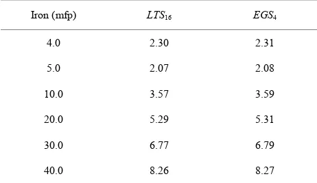
Here the exposure build-up factor is defined as the sum of the product of the attenuation coefficient of the air with the scalar flux for all photons, including the incident flux, divided by the attenuation coefficient of the air for the in- cident flux multiplied by the incident scalar flux. The nu- merical results for three problems are shown in Table 1

for water and lead, in Table 2 for water and iron and in

Table 3 for lead and iron. In Table 1 we present the

LTSN numerical simulations for the exposure build-up factor and comparisons with results from the EGS4 code

[7] generated for the one-group model. We consider a multi-layered slab with two regions, composed of water (μij = 0.0707 cm2/g and 1.0 mpf) and lead (μij = 0.06848 cm2_{/g and depth in multiples of the mean free path, 4.0,}

[image:4.595.307.538.598.732.2]

5.0, 10.0, 20.0, 30.0 and 40.0 mfp) together with the afore mentioned vacuum boundary conditions.

Table 1. Numerical exposure buildup factor simulations for a multilayered slab composed of water (1.0 mfp) and lead.

Iron (mfp) LTS16 EGS4

[image:5.595.56.288.112.245.2]

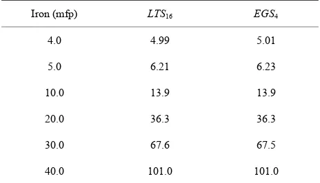
Table 2. Numerical exposure buildup factor simulations for a multilayered slab composed of water (1.0 mfp) and iron.

Iron (mfp) LTS16 EGS4

[image:5.595.55.287.284.423.2]

4.0 4.99 5.01 5.0 6.21 6.23 10.0 13.9 13.9 20.0 36.3 36.3 30.0 67.6 67.5 40.0 101.0 101.0

Table 3. Numerical exposure buildup factor simulations for a multilayered slab composed of lead (1.0 mfp) and iron.

Iron (mfp) LTS16 EGS4

4.0 4.87 4.86 5.0 6.34 6.28 10.0 15.4 15.3 20.0 41.5 41.4 30.0 78.4 78.3 40.0 118.0 117.0

In Table 2 we present the LTSN numerical simulations

for the exposure build-up factor and comparisons with the results from EGS4 generated for the one-group model.

We consider a multi-layered slab with two regions, composed of water (μij = 0.0707 cm2/g with depth of 1.0 mpf) and iron (μij = 0.0596 cm2/g with depth 4.0, 5.0, 10.0, 20.0, 30.0 and 40.0 mfp) and vacuum boundary con- ditions.

From the analysis of the results encountered in Tables 1-3, one realizes a fairly good agreement between the

LTS16 and EGS4 results. The numerical convergence of

the LTSN results showed for increasing N a coincidence of six significant digits for N = 14 and N = 16. For two-dimensional problems for photons and electrons, we applied the LTSN method, for N = 8, in the transport equation for photons and used N = 9 in the PN approxi-mation for the angular variable of the Fokker-Planck equa- tion for electrons. We considered homogeneous rectangu- lar geometries composed of water liquid (Z/A = 0.55508,

ρ = 1 g/cm2_{), soft tissue (ICRU44, Z/A = 0.54996, ρ =}

1.06 g/cm2_{) and cortical bone (ICRU44, Z/A = 0.51478, ρ}

= 1.92 g/cm2_{). Further, we assumed a mono-energetic (E}

= 1.25 MeV) and monodirectional photon beam incident on the edge of a rectangle with dimension 20 cm × 20 cm and vacuum boundary conditions. The incoming photons

were tracked until their whole energy was deposited and/ or they left the domain of interest. In this problem also the energy deposited by the secondary electrons, gener- ated by the Compton Effect, were considered. Other pos- sible effects, however with small or spurious contributions were not taken into account. The numerical results en- countered for absorbed energy in the domain were com- pared with simulations obtained with the program Geant4 v8 [8], using the low energy libraries and are presented in

Tables 4 and 5.

The numerical convergence of the LTSN results showed for increasing N a coincidence of three significant digits for N = 4, 6 and 8. Notice, the coincidence of four sig- nificant digits for the PN approximation with N = 7 and 9. These results were obtained in the homogeneous domain with dimension 20 cm × 20 cm that was composed of water. In Table 4 we present the LTS8 nodal numerical

simulations for the absorbed energy induced by photons incident on a homogeneous rectangular domain, that is composed of a variety of different materials. In Table 5

we present numerical simulations for absorbed energy by the P9 approximation, due to free electrons, arising from

Compton scattering in a homogeneous rectangular do- main composed of different materials. These results were compared with simulations obtained by Geant4.

In spite of the fact, that two different methods were used to simulate energy deposition, the Monte Carlo me- thod with Geant4 and our closed form solution the results

in Tables 4 and 5 show a fairly good agreement. From

[image:5.595.308.538.556.622.2]

the results, we notice that the maximum discrepancy found is 3.4% in the simulations for photons and 8.3% for electrons. The difference of our numerical results in comparison to the Geant simulations, that contain a cata- logue of processes, demonstrate that other effects shall be taken into account. As the material density increases, the Table 4. Absorved energy (KeV/photon emitted from the source) by the photons incident in a homogeneous domain dimension 20 cm × 20 cm, composed of materials different.

Domain composition LTSN Geant4 Discrepancy (%) Water liquid 0.00457 0.00468 2.3

[image:5.595.309.538.672.736.2]

Soft tissue 0.00531 0.00542 2.0 Cortical bone 0.0987 0.09487 3.4

Table 5. Absorved energy (KeV/photon emitted from the source) by the free electrons in a homogeneous domain di-mension 20 cm × 20 cm, composed of materials different.

Domain composition LTSN Geant4 Discrepancy (%) Water liquid 0.03379 0.03609 6.4

number of interactions increases as well as the possibility of other production processes involving secondary elec- trons, responsible for more than 86% of the total energy absorbed in domain.

5. Conclusion

Concluding, we were successful in determinig the LTSN solution in closed form forenergy deposition induced by photons in Cartesian geometry. From the solution we ob- tained the buildup factor and absorbed energy, for pho-tons and electrons, in the Compton energy range. It is worth mentioning, that the LTSN procedure maintains an analytical character of the solution and the unique appro- ximation made was in the leakage angular flux at the boundary. The PN solution of the Fokker-Planck equation remains analytical in the sense that no approximation is made along its derivation from PN equations, except for the truncation. Finally, a variety of additional numerical experiments have shown us that the presented method is robust for problems of the considered transport equation type.

6. Acknowledgements

The authors are gratefully to CNPq (Conselho Nacional de Desenvolvimento Científico e Tecnológico) for the partial financial support of this work. A special acknow- ledgment for the project INCT (Instituto Nacional de Ci- encia e Tecnologia—Reatores Nucleares Inovadores) for financial support.

REFERENCES

[1] C. F. Segatto, M. T. Vilhena and R. P. Pazos, “On the Con- vergence of the Spherical Harmonics Approximations,” Nu-clear Science and Engineering, Vol. 134, No. 1, 2000, pp. 114-119.

[2] M. T. Vilhena, C. F. Segatto and L. B. Barichello, “A Par- ticular Solution for the SN Radiative Transfer Problems,” Journal of Quantitative Spectroscopy and Radiative Tran- sfer, Vol. 53, No. 4, 1995, pp. 467-469.

doi:10.1016/0022-4073(95)90020-9

[3] C. Borges and E. W. Larsen, “The Transversely Inte- grated Scalar Flux of a Narrowly Focused Particle Beam,” SIAM Journal on Applied Mathematics, Vol. 55, No. 1, 1995, pp. 1-22.

[4] C. Borges and E. W. Larsen, “On the Accuracy of the Fokker-Planck and Fermi Pencil Beam Equation for Charged Particle Transport,” Medical Physics, Vol. 23, No. 10, 1996, pp. 1749-1759. doi:10.1118/1.597832 [5] B. D. A. Rodriguez, M. T. Vilhena, V. Borges and G. Hoff,

“A Closed Form Solution for the Two-Dimensional Fok-ker-Planck Equation for Electron Transport in the Range of Compton Effect,” Annals of Nuclear Energy, Vol. 35, No. 5, 2008, pp. 958-962.

doi:10.1016/j.anucene.2007.09.002

[6] B. D. A. Rodriguez, M. T. Vilhena and V. Borges, “A So- lution for the Two-Dimensional Transport Equation for Photons and Electrons in a Rectangular Domain by the Laplace Transform Technique,” International Journal of Nuclear Energy Science and Technology, Vol. 5, No. 1, 2010, pp. 25-40. doi:10.1504/IJNEST.2010.030304 [7] H. Hirayama and K. Shin, “Application of the EGS4 Monte

Carlo Code to a Study of Multilayer Gamma-Ray Expo- sure Buildup Factors,” Journal of Nuclear Science and Technology, Vol. 35, No. 11, p. 816.

doi:10.3327/jnst.35.816

[8] D. H. Wright, “Physics Reference Manual,” 2001. http://cern.ch/geant4

[9] G. C. Pomraning, “Flux-Limited Diffusion and Fokker- Planck Equations,” Nuclear Science and Engineering, Vol. 85, No. 2, 1983, p. 116.

[10] J. Wood, “Computational Methods in Reactor Shielding,” Pergamon Press, Oxford, 1982.

[11] S. Agostinelli, et al., “Geant4: A Simulation Toolkit,” Nu- clear Instruments and Methods in Physics Research A, Vol. 506, No. 3, 2003, pp. 250-303.

[12] DOORS 3.1, “One, Two and Three Dimensional Discrete Ordinates Neutron Photon Transport Code System,” Ra- diation Safety Information Computational Center (RSICC), Code Package CCC-650, Oak Ridge, Tennessee, 1996. [13] B. D. A. Rodriguez, M. T. Vilhena and V. Borges, “The

Determination of the Exposure Buildup Factor Formula- tion in a Slab Using the LTSN Method,” Kerntechnik, Vol.