Exploiting GPU Hardware Saturation for Fast Compiler Optimization

Exploiting GPU Hardware Saturation for Fast Compiler

Optimization

Alberto Magni

[email protected]

Christophe Dubach

[email protected]

Michael O’Boyle

[email protected]

ABSTRACT

Graphics Processing Units (GPUs) are efficient devices capa-ble of delivering high performance for general purpose com-putation. Realizing their full performance potential often requires extensive compiler tuning. This process is partic-ularly expensive since it has to be repeated for each target program and platform.

In this paper we study the utilization of GPU hardware re-sources across multiple input sizes and compiler options. In

this context we introduce the notion of hardwaresaturation.

Saturation is reached when an application is executed with a number of threads large enough to fully utilize the available hardware resources. We give experimental evidence of hard-ware saturation and describe its properties using 16 OpenCL kernels on 3 GPUs from Nvidia and AMD. We show that in-put sizes that saturates the GPU show performance stability across compiler transformations.

Using the thread-coarsening transformation as an exam-ple, we show that compiler settings maintain their relative performance across input sizes within the saturation region. Leveraging these hardware and software properties we pro-pose a technique to identify the input size at the lower bound of the saturation zone, we call it Minimum Saturation Point (MSP). By performing iterative compilation on the MSP input size we obtain results effectively applicable for much large input problems reducing the overhead of tuning by an order of magnitude on average.

Categories and Subject Descriptors

D.3.4 [Programming languages]: Processors —

Compil-ers, Optimization

General Terms

Experimentation, Measurement, Performance

Keywords

OpenCL, GPGPU, iterative compilation, optimization

1.

INTRODUCTION

Graphic Processing Units (GPUs) are now widely used due to their ability to deliver high performance for a large class of parallel applications. Such devices are most suited to solve problems larger in size than traditional multicore CPUs, taking advantage of the hundreds of cores available. Writing efficient code for GPUs is challenging due to the complexity of the underlying parallel hardware. Achieving high levels of performance requires expensive tuning by the programmer either evaluating manually multiple code ver-sions or using semi-automatic tools. This effort has to be replicated for every target program and architecture. Given the variety of devices now available and the high rate of hardware update the tuning cost is a significant problem.

To reduce tuning time, application programmers often evaluate many different compiler or code transformations on problem sizes smaller than their target. The aim is to have quick feedback on what are the most effective optimization options. This methodology assumes that code transforma-tions that work well on a small problem size will work well on the larger target size. The testing input size must be chosen with care: too small and it might not match the behaviour of the larger target size, too large and it makes tuning too expensive. Finding the right input size on which to perform tuning is a crucial issue.

To tackle this problem we introduce the concept of

satu-ration of hardware resources for graphics processors.

Satu-ration is achieved when an application is run with an input

size (i.e. number of threads) sufficiently large to fully utilize

hardware resources. Programs running in such a region of the input size space usually scale according to the complexity of the problem and show performance stability across pro-gram optimizations. This means that code transformations effective for a small input size in the saturation zone are usually effective for very large input sizes too. We develop a search strategy that exploits the Minimum Saturation Point (MSP) to reduce reduce the total tuning time necessary to find good optimization settings.

In this work we describe the property of saturation in

terms of the throughput metric: the amount of work

per-formed by a parallel program per unit of time, showing how this reaches stability in the saturation zone. In summary the paper makes the following contributions:

• We show the existence of saturation for 16 OpenCL

benchmarks on three GPU architectures: Fermi and

Kepler by Nvidia andTahitiby AMD.

• We show that the hardware saturation can be

success-fully exploited to speedup iterative tuning of applica-tions leading to a reduction of search space of an order of magnitude.

The rest of the paper is organized as follows: section 2 motivates the problem with an example. Section 3 describes our experimental setup and section 4 introduces the con-cept of saturation point. Section 5 describes a technique to identify the lower bound of the saturation area using the throughput metric while section 6 presents detailed results. Section 7 presents the related work, finally section 8 con-cludes the paper.

2.

MOTIVATING EXAMPLE

This section introduces the problem by showing how an OpenCL program reacts when performing iterative compi-lation on multiple input sizes. As an example we use the

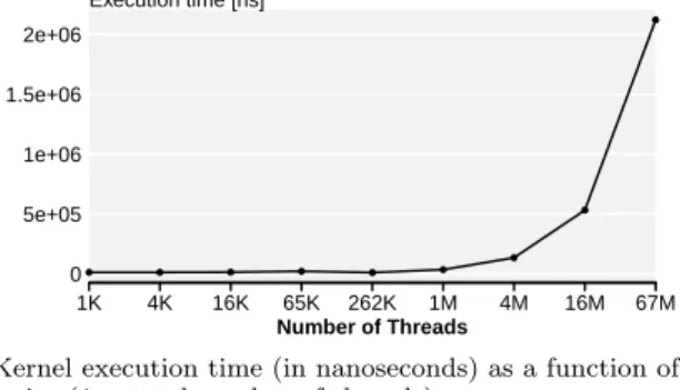
floydWarshallprogram running on the AMD Tahiti GPU and the optimization space of the thread coarsening trans-formation [6]. Figure 1 shows the behavior of our benchmark as a function of its input size. For OpenCL workloads there is direct mapping between the input size and the overall number of instantiated threads. We measure the problem size using the total number of instantiated threads.

Figure 1a shows the execution time of the application as

a function of the input size. The largest data size, with

67 million threads is the input size we want to optimize for. Unsurprisingly this leads to the longest execution time. If we were to tune this application by evaluating multiple versions, the time required to search the optimization space would be directly proportional to the execution time. As a results, it would be preferable to tune the application on the smallest possible input size.

However, the performance of the best optimization

set-tings for a given problem size does not transfer across all

input sizes as shown in figure 1b. The best optimization settings for the smallest input size achieves only a third of the performance of the best one corresponding to the largest input size. This means, that if the application were tuned for the smallest input size, it would run three times slower than the best achievable on the large input size. A good trade-off is an input size of 1M threads achieving perfor-mance within few percents of the largest input size. This

represents a savings of 67×in search time (67M/1M). The

question is how can we find the optimal input size without having to conduct the search for all input sizes in first place. One way to solve this problem is to look at the through-put metric, which is typically expressed as the number of operations executed per second (the formal definition of this metric is given in section 4). Figure 1c shows the throughput of the application as a function of the problem size. As can be seen, the throughput starts very low and increases with the problem size. It flattens out at around 4M threads which corresponds to the saturation of the hardware resources. We

call this point theminimum saturation point (MSP), given

that passed this point throughput remains constant. Coin-cidentally, the MSP is smaller than the target input size and leads to performance on par with the best achievable when searching on the largest input size.

● ● ● ● ● ● ● ● ● 0 5e+05 1e+06 1.5e+06 2e+06 Execution time [ns] 1K 4K 16K 65K 262K 1M 4M 16M 67M Number of Threads

(a) Kernel execution time (in nanoseconds) as a function of the input size (i.e.total number of threads).

Performance 0 0.2 0.4 0.6 0.8 1 1K 4K 16K 65K 262K 1M 4M 16M 67M Number of Threads

(b)Normalized performance attaibable when performing the tuning on a given input size and evaluating the best performing configuration found on the largest one (67M). For example the best performing configuration for input size 1K achieves only 30% of the maximum attainable by tuning coarsening directly on input size 67M. 0 5 10 15 20 25 30 ● ● ● ● ● ● ● ● ● Throughput 1K 4K 16K 65K 262K 1M 4M 16M 67M Number of Threads

(c)Throughput as a function of the problem input size.

Figure 1. Execution time a, relative performance b and

throughput c of the program floydWarshall running on

AMD Tahiti as a function of the input size (expressed as

total number of threads). Notice the log-scale of the x-axes.

The remainder of the paper characterizes hardware satu-ration using the throughput metric and shows that it can be used successfully to reduce tuning time.

3.

EXPERIMENTAL SETUP

3.1

Benchmarks and Platforms

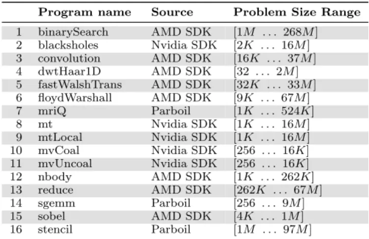
In this paper, we use 16 OpenCL benchmarks from vari-ous sources, as shown in Table 1. In the case of programs

from theParboil benchmark suite we used theopencl base

version. The table reports the range of sizes for the input problem, these are reported in terms of the total number of launched threads. For the rest of the paper we will consider

the largest problem size as the target one,i.e. the one that

plat-Program name Source Problem Size Range 1 binarySearch AMD SDK [1M . . . 268M] 2 blacksholes Nvidia SDK [2K . . . 16M] 3 convolution AMD SDK [16K . . . 37M] 4 dwtHaar1D AMD SDK [32 . . . 2M] 5 fastWalshTrans AMD SDK [32K . . . 33M] 6 floydWarshall AMD SDK [9K . . . 67M] 7 mriQ Parboil [1K . . . 524K] 8 mt Nvidia SDK [1K . . . 16M] 9 mtLocal Nvidia SDK [1K . . . 16M] 10 mvCoal Nvidia SDK [256 . . . 16K] 11 mvUncoal Nvidia SDK [256 . . . 16K] 12 nbody AMD SDK [1K . . . 262K] 13 reduce AMD SDK [262K . . . 67M] 14 sgemm Parboil [256 . . . 9M] 15 sobel AMD SDK [4K . . . 1M] 16 stencil Parboil [1M . . . 97M]

Table 1. OpenCL programs with the range of input sizes used for our experiments

Name Model GPU OpenCL Linux

Driver version kernel Tahiti AMD Tahiti 7970 1084.4 1.2 SDK 1084.4 3.1.10 Fermi Nvidia GTX 480 304.54 1.1 CUDA 5.0.1 3.2.0 Kepler Nvidia K20c 331.20 1.1 CUDA 5.0.1 3.7.10

Table 2. OpenCL devices used for our experiments.

forms described in Table 2. In all our experiments we only measure the kernel execution time. To reduce measurement noise each experiment has been repeated 50 times aggregat-ing the results usaggregat-ing the median.

3.2

Optimization Space

The parameters of the thread-coarsening transformation

define our search space. Coarsening can be thought as loop unrolling for the OpenCL parallel loop. It works by increas-ing the amount of work performed by a sincreas-ingle thread by merging multiple threads of the original application and con-sequently reducing the overall number of running threads. As a convention, for the remainder of the paper we refer to input size the number of threads of the original uncoarsened application. Coarsening is controlled by a three parameters:

• factor: define how many threads to merge together,

i.e. by how much to reduce the thread space,

• stride: define how to remap threads after the

transfor-mation so to preserve coalescing of memory accesses,

• local–work–group size: define how many threads are

scheduled concurrently onto a single core.

We tuned the transformation by considering all combination of our parameters leading to about 150-300 configurations for one dimensional kernels and 1000-2000 configuration for two dimensional kernels depending on the device limitation and the problem size. These add up to about 160000 config-urations evaluated across all input sizes, programs and de-vices. This large evaluation of the coarsening transformation is made possible by the our portable compiler toolchain [6].

4.

THROUGHPUT AND HARDWARE

SATURATION

This section defines the concept of hardware saturation and presents its features.

Graphics processors are highly parallel machines contain-ing a large amount of computcontain-ing cores. To harness the com-puting power of GPUs applications must run large amount of threads to fully exploit all the hardware resources. Pro-grams running a small number of threads might show a be-havior which is not representative of larger ones due to un-der utilization of the hardware resources. We describe this behavior using the notion of throughput which we formally defined as :

throughput= units of work

execution time (1)

where units of workis a metric which depends on the

al-gorithmic complexity of the application. In case of linear benchmarks, this corresponds to the number of input

ele-ments processed by the kernel : units of work=input size.

In case of non-linear programs the input size is scaled

accord-ing to the complexity. For example the nbody program is

quadratic in complexity andunits of work= (input size)2.

Note that in our benchmarks the total number of threads is

a linear function of theinput size.

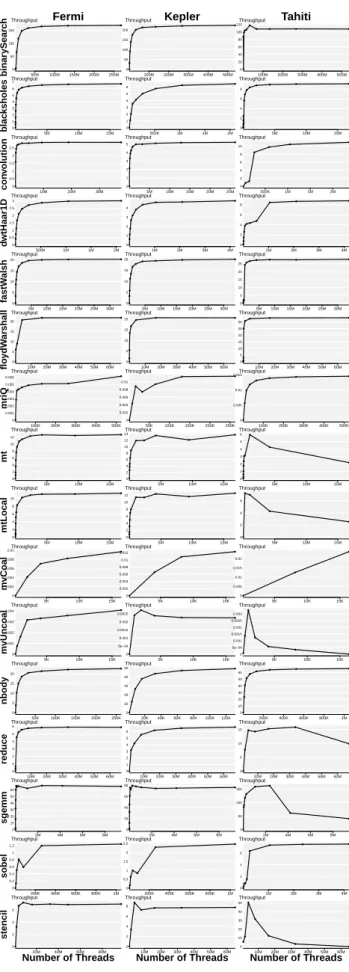
Figure 2 shows the throughput as a function of the to-tal number of running threads for each benchmark and our three platforms. Consider, for example, the first plot in

fig-ure 2,binarySearchrunning onFermi. This graph clearly

shows that the throughput increases along with the problem

size (i.e. total number of threads) until 50 million threads.

Passed this size the throughput reaches a plateau and

sta-bilizes at around 180 billionunits of workper second. We

call this region of the input space saturation region. From

the shape of the plot we can make two observations. The first one is that a program run with a small number of threads does not behave in the same way as with a large number. In particular small input sizes are in proportion slower than large ones, showing very low throughput val-ues. Second, the fact that the throughput stabilizes for suf-ficiently large input sizes shows that we hit the hardware saturation limit of the GPUs and that applications scale close to the theoretical algorithmic complexity.

4.1

Outliers Analysis

TheTahiti column in figure 2 shows a number of outliers

which do not show a plateau. Examples of these are:

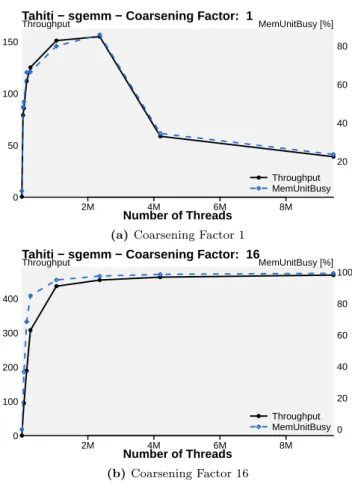
mvUn-caol,sgemm,stencil,mtandmtLocal. Notice that all these programs are memory bound. We investigate these cases us-ing performance counters. Figure 4 reports the results of our

analysis for sgemm. The top sub-figure shows the

through-put performance along with the value of the performance

counterMemUnitBusy as a function of the total number of

threads. MemUnitBusy is the hardware counter that

mea-sures the percentage of execution time that the memory unit is busy processing loads and stores. We can see that there is a very high correlation between the two curves. This sig-nifies that performance for large input sizes is limited by the memory functional unit, which is unable to handle ef-ficiently a large amount of requests coming from different threads. As shown in figure 4b the coarsening transforma-tion mitigates this problem, leading to much higher per-formance. The throughput curve still follows the hardware

0 50 100 150 ●● ● ● ● ● ● ● ● Throughput 50M 100M 150M 200M 250M binar ySear c h Fermi 0 50 100 150 200 ● ● ● ● ● ● ● ● ● ● Throughput 100M 200M 300M 400M 500M Kepler 0 20 40 60 80 100 120 ● ● ● ●● ● ● ● ● ● Throughput 100M 200M 300M 400M 500M Tahiti 0 1 2 3 4 5 6 7 ● ● ● ● ● ● ● ● ● ● ● ● ● ● Throughput 5M 10M 15M b lac ksholes 0 1 2 3 4 5 6 ● ● ● ● ● ● ● ● ● Throughput 500K 1M 1M 2M 0 2 4 6 8 ●● ● ● ● ● ● ● ● ● ● ● ● ● ● Throughput 5M 10M 15M 0 0.5 1 1.5 2 2.5 ● ● ● ● ●● ●● ● ● ● Throughput 10M 20M 30M con v olution 0 1 2 3 4 5 ● ● ● ● ● ● ●● ● ● ● Throughput 5M 10M 15M 20M 25M 0 2 4 6 8 10 ● ●● ● ● ● ● Throughput 500K 1M 1M 2M 0 0.5 1 1.5 2 2.5 3 ● ● ● ● ● ● ● ● ● ● ● Throughput 500K 1M 1M 2M d wtHaar1D 0 1 2 3 4 ● ● ● ● ● ● ● ● ● ● ● Throughput 1M 2M 3M 4M 0 2 4 6 8 ●● ● ● ● ● ●● ● ● ● ● Throughput 1M 2M 3M 4M 0 5 10 15 20 ● ● ● ● ● ● ● ● ● ● ● Throughput 5M 10M 15M 20M 25M 30M fastW alsh 0 5 10 15 20 ● ● ● ● ● ● ● ● ● ● ● Throughput 5M 10M 15M 20M 25M 30M 0 5 10 15 20 25 ● ●●● ● ●● ● ● ● ● Throughput 5M 10M 15M 20M 25M 30M 0 5 10 15 20 ● ● ● ● ● ● Throughput 10M 20M 30M 40M 50M 60M flo ydW ar shall 0 5 10 15 20 ● ● ● ● ● ● ● ● Throughput 10M 20M 30M 40M 50M 60M 0 5 10 15 20 25 30 ●●● ● ● ● ● ● ● Throughput 10M 20M 30M 40M 50M 60M 0 0.001 0.002 0.003 0.004 0.005 0.006 ● ● ● ● ● ● ● ● ● Throughput 100K 200K 300K 400K 500K mriQ 0 0.002 0.004 0.006 0.008 0.01 ● ● ● ● ● ● ● Throughput 50K 100K 150K 200K 250K 0 0.005 0.01 0.015 ● ● ● ● ● ● ● ● Throughput 100K 200K 300K 400K 500K 0 2 4 6 8 10 12 ● ● ● ● ● ● ● ● ● ● ● ● ● Throughput 5M 10M 15M mt 0 2 4 6 8 10 12 14 ● ● ● ● ● ● ● ● ● ● ● Throughput 5M 10M 15M 0 1 2 3 4 5 6 ● ● ● ● ● ● ●● ● ● ● Throughput 5M 10M 15M 0 2 4 6 8 10 ● ●● ● ● ● ● ● ● ● ● ● ● Throughput 5M 10M 15M mtLocal 0 2 4 6 8 10 12 ● ● ● ● ● ● ● ● ● ● ● ● Throughput 5M 10M 15M 0 2 4 6 ● ●● ● ● Throughput 5M 10M 15M 0 0.002 0.004 0.006 0.008 0.01 ● ● ● ● ● Throughput 5K 10K 15K mvCoal 0 0.002 0.004 0.006 0.008 0.01 0.012 ● ● ● ● Throughput 5K 10K 15K 0 0.005 0.01 0.015 0.02 ● ● ● Throughput 5K 10K 15K 0 0.001 0.002 0.003 0.004 ● ● ● ● ● ● ● Throughput 5K 10K 15K mvUncoal 0 5e−04 0.001 0.0015 0.002 0.0025 ● ● ● ● ● ● Throughput 5K 10K 15K 0 5e−04 0.001 0.0015 0.002 0.0025 0.003 ● ● ● ● ● ● ● Throughput 5K 10K 15K 0 5 10 15 20 ● ● ● ● ● ● ● ● ● Throughput 50K 100K 150K 200K 250K nbod y 0 10 20 30 40 50 ● ● ● ● ● ● ● Throughput 20K 40K 60K 80K 100K 120K 0 10 20 30 40 50 60 ● ● ● ● ● ● ● ● ● Throughput 200K 400K 600K 800K 1M 0 1 2 3 4 5 6 ● ● ● ● ● ● ● ● ● ● Throughput 10M 20M 30M 40M 50M 60M reduce 0 1 2 3 4 5 6 ● ● ● ● ● ● ● Throughput 10M 20M 30M 40M 50M 60M 0 5 10 15 ● ● ● ● ● ● ● Throughput 10M 20M 30M 40M 50M 60M 0 10 20 30 40 50 60 ● ● ● ● ● ● ●●● ● ● ● ● Throughput 2M 4M 6M 8M sg emm 0 20 40 60 80 ●● ● ● ● ● ● ● ●●● ● ● ● Throughput 2M 4M 6M 8M 0 50 100 150 ● ● ● ● ● ● ● ● ● Throughput 2M 4M 6M 8M 0 0.2 0.4 0.6 0.8 1 1.2 ● ● ● ● ● ● ● Throughput 200K 400K 600K 800K 1M sobel 0 0.5 1 1.5 2 2.5 ● ● ● ● ● ● ● Throughput 200K 400K 600K 800K 1M 0 2 4 6 ● ● ●● ● ● ● ● ● Throughput 1M 2M 3M 4M 0 2 4 6 ● ● ● ● ● ● ● ● Throughput 20M 40M 60M 80M stencil Number of Threads 0 2 4 6 8 ● ● ● ● ● ● ● Throughput 10M 20M 30M 40M 50M 60M Number of Threads 0 10 20 30 40 50 ● ● ● ● ● ● ● Throughput 10M 20M 30M 40M 50M 60M Number of Threads

Figure 2. Throughput, defined as billions units of work processed per unit of time (see formula 1), as a function of

the total number of threads (i.e. the problem input size) for

all the programs and the three devices.

0 0.2 0.4 0.6 0.8 1●●● ●●● ● ● ● Performance 50M 100M 150M 200M 250M binar ySear c h Fermi 0 0.2 0.4 0.6 0.8 1 ●● ● ● ●● ● ● ● ● Performance 100M 200M 300M 400M 500M Tahiti 0 0.2 0.4 0.6 0.8 1 ●● ● ● ● ● ● ● ● ● Performance 100M 200M 300M 400M 500M Kepler 0 0.2 0.4 0.6 0.8 1 ● ●● ● ● ● ●● ●● ● ● ● ● Performance 5M 10M 15M b lac ksholes 0 0.2 0.4 0.6 0.8 1 ● ● ● ● ●● ● ●● ●● ● ● ● ● Performance 5M 10M 15M 0 0.2 0.4 0.6 0.8 1 ● ● ●●●● ● ● ● Performance 500K 1M 1M 2M 0 0.2 0.4 0.6 0.8 1●●● ●●●● ● ● ● ● Performance 10M 20M 30M con v olution 0 0.2 0.4 0.6 0.8 1 ● ●● ● ● ● ● Performance 500K 1M 1M 2M 0 0.2 0.4 0.6 0.8 1 ● ●●●● ●●● ● ● ● Performance 5M 10M 15M 20M 25M 0 0.2 0.4 0.6 0.8 1 ● ● ● ● ●● ● ● ● ● Performance 500K 1M 1M 2M d wtHaar1D 0 0.2 0.4 0.6 0.8 1 ● ● ●●● ● ● ● ● ● ● ● Performance 1M 2M 3M 4M 0 0.2 0.4 0.6 0.8 1 ● ● ●● ● ●● ● ● ● Performance 1M 2M 3M 4M 0 0.2 0.4 0.6 0.8 1 ● ●● ● ● ●● ● ● ● ● Performance 5M 10M 15M 20M 25M 30M fastW alsh 0 0.2 0.4 0.6 0.8 1●●● ● ● ●● ● ● ● ● Performance 5M 10M 15M 20M 25M 30M 0 0.2 0.4 0.6 0.8 1 ● ●●●●●●● ● ● ● Performance 5M 10M 15M 20M 25M 30M 0 0.2 0.4 0.6 0.8 1 ● ● ●● ● ● Performance 10M 20M 30M 40M 50M 60M flo ydW ar shall 0 0.2 0.4 0.6 0.8 1 ●● ●●● ●● ● ● Performance 10M 20M 30M 40M 50M 60M 0 0.2 0.4 0.6 0.8 1 ● ● ● ● ● ● ● ● Performance 10M 20M 30M 40M 50M 60M 0 0.2 0.4 0.6 0.8 1 ●●● ● ● ● ● ● ● Performance 100K 200K 300K 400K 500K mriQ 0 0.2 0.4 0.6 0.8 1 ● ● ●● ● ● ● ● Performance 100K 200K 300K 400K 500K 0 0.2 0.4 0.6 0.8 1 ● ● ● ● ● ● ● Performance 50K 100K 150K 200K 250K 0 0.2 0.4 0.6 0.8 1 ● ●● ● ● ● ● ●● ● ● ● ● Performance 5M 10M 15M mt 0 0.2 0.4 0.6 0.8 1 ●● ●● ● ●● ● ● ● ● Performance 5M 10M 15M 0 0.2 0.4 0.6 0.8 1 ● ●● ● ● ● ● ● ● ● ● Performance 5M 10M 15M 0 0.2 0.4 0.6 0.8 1 ● ● ● ● ● ● ● ● ● ● ● ● ● Performance 5M 10M 15M mtLocal 0 0.2 0.4 0.6 0.8 1 ● ● ● ● ● Performance 5M 10M 15M 0 0.2 0.4 0.6 0.8 1 ● ● ● ● ● ● ● ● ● ● ● ● Performance 5M 10M 15M 0 0.2 0.4 0.6 0.8 1 ● ● ● ● ● Performance 5K 10K 15K mvCoal 0 0.2 0.4 0.6 0.8 1● ● ● Performance 5K 10K 15K 0 0.2 0.4 0.6 0.8 1 ● ● ● ● Performance 5K 10K 15K 0 0.2 0.4 0.6 0.8 1● ● ●● ● ● ● Performance 5K 10K 15K mvUncoal 0 0.2 0.4 0.6 0.8 1 ● ●● ●●● ● ● Performance 100K 200K 300K 0 0.2 0.4 0.6 0.8 1 ● ● ● ● ● ● Performance 5K 10K 15K 0 0.2 0.4 0.6 0.8 1● ●● ●●● ● ● ● Performance 50K 100K 150K 200K 250K nbod y 0 0.2 0.4 0.6 0.8 1 ● ●● ●● ● ● ● ● Performance 200K 400K 600K 800K 1M 0 0.2 0.4 0.6 0.8 1● ●● ● ● ● ● Performance 20K 40K 60K 80K 100K 120K 0 0.2 0.4 0.6 0.8 1●●● ● ●●● ● ● ● Performance 10M 20M 30M 40M 50M 60M reduce 0 0.2 0.4 0.6 0.8 1● ●● ● ● ● ● Performance 10M 20M 30M 40M 50M 60M 0 0.2 0.4 0.6 0.8 1● ●● ● ● ● ● Performance 10M 20M 30M 40M 50M 60M 0 0.2 0.4 0.6 0.8 1 ●● ●●● ● ● ● ● ● ● ● ● Performance 2M 4M 6M 8M sg emm 0 0.2 0.4 0.6 0.8 1 ●●● ● ● ● ● ● ● Performance 2M 4M 6M 8M 0 0.2 0.4 0.6 0.8 1 ● ●●●● ● ● ●● ●● ● ● ● Performance 2M 4M 6M 8M 0 0.2 0.4 0.6 0.8 1● ● ●● ● ● ● Performance 200K 400K 600K 800K 1M sobel 0 0.2 0.4 0.6 0.8 1● ● ● ● ● ● ● ● ● Performance 1M 2M 3M 4M 0 0.2 0.4 0.6 0.8 1 ●● ● ● ● ● ● Performance 200K 400K 600K 800K 1M 0 0.2 0.4 0.6 0.8 1 ● ● ● ● ● ● ● ● Performance 20M 40M 60M 80M stencil Number of Threads 0 0.2 0.4 0.6 0.8 1 ● ● ● ● ● ● ● Performance 10M 20M 30M 40M 50M 60M Number of Threads 0 0.2 0.4 0.6 0.8 1 ● ● ● ● ● ● ● Performance 10M 20M 30M 40M 50M 60M Number of Threads

Figure 3. Performance of the best optimizations settings found for a given input size evaluated on the largest input size.

0 50 100 150 ● ● ● ● ● ● ● ● ● Throughput

Tahiti − sgemm − Coarsening Factor: 1

2M 4M 6M 8M

Number of Threads_globalSize

v alues 20 40 60 80 MemUnitBusy [%] ● _Throughput MemUnitBusy

(a) Coarsening Factor 1

0 100 200 300 400 ● ● ● ● ● ● ● ● Throughput

Tahiti − sgemm − Coarsening Factor: 16

2M 4M 6M 8M

Number of Threads_globalSize

v alues 0 20 40 60 80 100 MemUnitBusy [%] ● _Throughput MemUnitBusy (b)Coarsening Factor 16

Figure 4. Correlation between throughput and

MemUnit-Busyhardware counter forsgemmonTahitiusing coarsening

factor 1 and 16. MemUnitBusy is the percentage of time in

which the memory unit is busy processing memory requests. We can see that the coarsened configuration does not suffer of low memory utilization leading much higher throughput.

counter without dropping for higher input sizes. A similar

analysis can be performed for programs such as mvUncoal

where the uncoalesced memory access pattern highlights the

problem even more. ThemvUncoalbenchmark is described

in more detail in section 6.

5.

THROUGHPUT-BASED TUNING

Taking advantage of the saturation properties described earlier, this section introduces a methodology to accelerate iterative compilation.

5.1

Tuning Across Input Sizes

We now show how the best compiler settings found for a given input size perform on the largest input size. Figure 3 shows this performance on all benchmarks and devices for the full compiler transformation space described in section 3.

For example a value of 1 for input size x means that the

best performing coarsening configuration forxis the best for

the target size as well. A value of 0.5 means that the best

configuration onxgives half of the maximum performance

when evaluated on the target. By definition the line reaches 1 for the largest input size.

0 10 20 30 40 1 2 4 8 ● ● ● ● ● 16● 32 Throughput floydWarshall 9K 262K 1M 4M 16M 67M Number of Threads

Figure 5. Throughput as a function of problem input size

(i.e. the total number of threads) for five different values of

the coarsening factor (on the right) for floydWarshallon

Kepler. Note the log-scale of the x-axis, this to highlight

the throughput of small input sizes.

The overall trend for performance is to increase as the tuning input size gets close to the target one. After a cer-tain input size, performance reaches a plateau and stabilizes in most cases. Small input sizes tends to have low and un-predictable performance while large input sizes have perfor-mance close to that of the largest input size. This means that for input sizes in that saturate the device performance reaches stability. This can be clearly seen when compar-ing figure 2 and 3; when throughput saturates, so does the performance.

5.2

Throughput and Coarsening Factor

Before introducing our search technique, we consider the impact of the thread coarsening factor on the throughput as shown in figure 5. This figures shows the throughput for five different values of the factor parameter for the coarsen-ing transformations (labeled on the right). The relative per-formance of the different coarsening factors changes across input sizes until saturation is reached between 1M and 4M threads. For all coarsening factors, the throughput reaches a plateau and stabilizes after 1M threads. In this example the factors 8 and 16 are the best parameters for problem sizes of about 4 million threads remaining stable up to 67 million threads.

This signifies that performing a search for the best param-eter at the left of the saturation point will probably lead to bad choices when evaluating on the largest input size. On the contrary, performing beyond the saturation should lead to good choices when evaluated on the largest input size.

5.3

Throughput Based Input Size Selection

We now propose a tuning technique that takes advantage of the saturation plateau that exists for both performance and throughput. We first build the throughput curve by (1) running the benchmark using the default compiler parame-ters on multiple input sizes within the range given in table 1. Once the throughput curve is built, (2) we select the smallest input size that achieves a throughput within a given thresh-old of the maximum one. The threshthresh-old is used to deal with noise in the experimental data and small fluctuations in ex-ecution time around the throughput plateau. The resulting selected input size is our Minimum Saturation Point (MSP)

Program name Fermi Kepler Tahiti 1) binarySearch 8M 16M 8M 2) blacksholes 1M 1M 1M 3) convolution 262K 802K 1M 4) dwtHaar1D 262K 524K 1M 5) fastWalshTrans 2M 2M 1M 6) floydWarshall 4M 4M 1M 7) mriQ 524K 131K 65K 8) mt 2.3M 4M 1M 9) mtLocal 1M 1M 262K 10) mvCoal 16K 16K 16K 11) mvUncoal 16K 1K 1K 12) nbody 32K 65K 131K 13) reduce 1M 1M 2M 14) sgemm 36K 65K 1M 15) sobel 262K 262K 1M 16) stencil 4M 4M 4M

Table 3. Minimum Saturation Point identified by the tech-nique presented in section 5 for all the benchmarks and ar-chitectures. MSP is expressed in number of threads.

and are presented in table 3 for all benchmarks and devices. The last step consist of (3) conducting the tuning or search at the MSP. Following this methodology, we expect that the best optimization settings found at the MSP leads to per-formance in par with the best for the largest input size. We refer to this searching technique as MSP-Tuning.

The next section presents the results obtained applying the proposed tuning technique.

6.

RESULTS

This section provides detailed results for the speedups in kernel execution time and in search time given by MSP-Tuning

6.1

Search Speedup Definition

In our experiments the baseline to compute kernel speedups is represented by the execution time of the application run

without applying the coarsening transformation (i.e.

coars-ening factor 1) and with the default local work group size by the benchmark suite. In all our experiments the prob-lem size we are optimizing for is the largest of the range

we record in table 1, we call this the target problem size.

Figure 6 summarizes the results of MSP-Tuning described in section 5 for our three OpenCL devices. Consider the top barplot in each subfigure. It reports the speedup over the baseline attainable using MSP-Tuning compared to the maximum speedup attainable with thread-coarsening. The second barplot reports the speedup in the search optimal configuration. The speedup is computed using this formula:

Search speedup= T imetarget

T imeM SP+T imethroughput

(2) HereT imetargetis the time spent exhaustively searching for

the best configuration on thetargetinput size,T imeM SP is

the search time on the MSP input size andT imethroughput

is the time spent building the throughput curve.

Maximum Speedup MSP-Tuning Speedup 0 1 2 3 4Speedup 1 5 10 50 100 500 1000 binar ySearch blacksholes con volution dwtHaar1D fastW alsh floydW arshall mr iQ mt mtLocal mvCoal mvUncoal

nbody reduce sgemm sobel stencil geoMean

Search time speedup

(a)Fermi 0 1 2 3 4Speedup 1 5 10 50 100 500 1000 binar ySearch blacksholes con volution dwtHaar1D fastW alsh floydW arshall mr iQ mt mtLocal mvCoal mvUncoal

nbody reduce sgemm sobel stencil geoMean

Search time speedup

(b)Kepler 0 1 2 3 4 Speedup 5.75.6 7.0 11.9 1 2 5 10 20 50 100 200 binar ySearch blacksholes con volution dwtHaar1D fastW alsh floydW arshall mr iQ mt mtLocal mvCoal mvUncoal

nbody reduce sgemm sobel stencil geoMean

Search time speedup

(c)Tahiti

Figure 6. Summary of the tuning results for the three architectures. In each subfigure, the top plot represents the kernel execution speedup attainable with MSP-Tuning in comparison with the maximum available speedup given by coarsening. The bottom plot shows the search-time speedup given by MSP-Tuning, notice that in this plot the y-axis is in log-scale.

6.2

Result Description

The kernel speedups achieved onFermi,KeplerandTahiti

are respectively: 1.35×, 1.24×and 1.55×. Which represent

82%, 73% and 53% of the maximum performance. On the other hand the search time speedup given by MSP-Tuning is about one order of magnitude for the three devices. To fully understand the savings results we have to take into account the algorithmic complexity of the application. A

program likesgemmensures very large tuning savings (even

in the order of thousands) thanks to its cubic complexity: halving the input size leads to a factor of eight in tuning time saving. The overall results are very similar for the two

Nvidia GPUs,FermiandKeplerdemonstrating the

similar-ities of the two architectures. On the other hand the Tahiti results show significant differences with higher speedups on average. The search fails to achieve good performance due onmtLocal,mvUncoalandstencildue to the erratic shape of throughput and performance lines for these benchmarks.

Of particular interest is the application mvCoal. This is

a matrix-vector multiplication benchmark from the Nvidia SDK. Considering the search time speedup barplots (and comparing tables 1 and 3) we can see that no reduction on

the input size is attainable, i.e. the selected MSP

corre-sponds to the largest input size. This is because no satu-ration plateau is reached, check the corresponding plot in figure 2. The reason for this behavior lies in the structure of the algorithm: one thread processes one row of the input matrix and the whole input vector producing a single ele-ment of the output. Thus we have only a thread for each matrix row: very few with respect to the complexity of the problem. Scaling the problem to larger sizes is prohibitive, running 16K threads means to work with about 1GB of data, scale to 32K means to work with 4GB, hitting device hard-ware constraints. In summary our target GPUs cannot full

express the throughput potential of mvCoal due to

limita-tions in the available memory resources. Similar

considera-tions can be made for mvUncoal, a different version of the

same program.

6.3

Noise Threshold

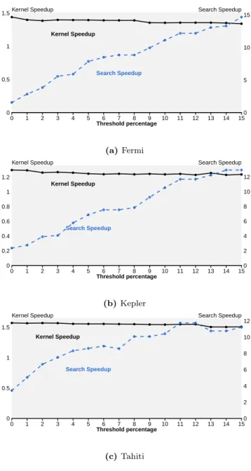
Figure 7 shows how the choice of the noise threshold de-scribed in section 5.3 affects the performance of our strat-egy. For the values of percentages between 0 and 15 it plots the achievable kernel speedup by implementing the search technique and the saving in search time. As expected the search speedup increases with the threshold percentage, this because the higher threshold values allows the selection of smaller input sizes as MSP. The kernel speedup slightly de-creases increasing the percentage. Based on this data, we se-lected a threshold of 10%, leading to marginal performance

degradation with respect to 0% and more than 10×

improve-ment in search speed across platforms.

7.

RELATED WORK

7.1

Performance Prediction for Parallel

Ap-plications and Systems

Reducing the cost of program tuning has been widely con-sidered in the literature. Yang et al. [10] concon-sidered running just a small fraction of a parallel application on a testing architecture using the results to tune it on a different one. Other works [4, 1] have made use of performance modeling.

0 0.5 1 1.5● ● ● ● ● ● ● ● ● ● ● ● ● ● ● ● 0 5 10 15

Kernel Speedup Search Speedup

0 1 2 3 4 5 6 7 8 9 10 11 12 13 14 15 Threshold percentage Search Speedup Kernel Speedup (a)Fermi 0 0.2 0.4 0.6 0.8 1 1.2 ● ● ● ● ● ● ● ● ● ● ● ● ● ● ● ● 0 2 4 6 8 10 12

Kernel Speedup Search Speedup

0 1 2 3 4 5 6 7 8 9 10 11 12 13 14 15 Threshold percentage Search Speedup Kernel Speedup (b)Kepler 0 0.5 1 1.5 ● ● ● ● ● ● ● ● ● ● ● ● ● ● ● ● 0 2 4 6 8 10 12

Kernel Speedup Search Speedup

0 1 2 3 4 5 6 7 8 9 10 11 12 13 14 15 Threshold percentage Search Speedup Kernel Speedup (c)Tahiti

Figure 7. Plots showing the attainable kernel speedup and the search-time speedup as a function of the noise threshold. A threshold of 0% means that we select the input size giving the maximum throughput. We can see that by increasing the threshold we can improve the search speedup with small degradation of the kernel speedup.

The first [4] predicts performance for various application-specific parameters such as working-set size and processors topology. The second [1] predicts the scalability of an appli-cation on a various number of processors. However, both techniques require significant amount of training and do not consider the problem of finding the hardware saturation point. Other researchers have looked at using techniques such as deterministic replay coupled with clustering to select representative replays [11]. A trace of the application is ex-tracted from a host machine and is then replayed locally on a single node. Interestingly, it is possible to use this technique to execute multiple replays on the same machine node in

or-der to estimate resource contention and predict performance of the whole system. This prior work has focused on extrap-olating performance of the whole system using just a few nodes. In our case, we are addressing a different problem,

i.e. determining what is the minimum application workload

that saturates the machine. Once this point has been found, we can use this to extrapolate performance on a larger input size problem.

Fursin and Chen [3, 2] have studied the sensitivity of opti-mizations to the program input for sequential applications. They have shown that it has little effect on the results of iterative compilations. This is a different conclusion from our results and is probably due to the benchmarks used (embedded programs) not stressing the underlying machines enough and the differences between sequential an parallel GPU hardware.

7.2

Optimization Space Exploration on GPUs

There has been a large amount of work dedicated to opti-mization space pruning. We focus on the most recent work applied to GPU compiler space optimization.

Ryoo et al. [8] developed an analytical model to predict the performance of compiler optimization for a CUDA architec-ture. Liue et al. [5] built a model to predict which optimiza-tion to apply for a given input size. While these approaches have the potential to speedup the exploration of the design space, they still rely on large data collection in order to build a model. Samadi et al. [9] have looked at using StreamIt and automatically generate optimised for high-level opera-tors such a reduction. They use a performance model to determine which version to use on the target system. Our technique is orthogonal to these since we present a method-ology to speed up empirical search of the optimization space by reducing the problem input size on which to perform the search. Finally, some recent work [7] looked at the effect on input size on the optimisation space. They use a simple clustering technique to group input-sizes based that share a common optimization configuration that lead to the best performance.

8.

CONCLUSION AND FUTURE WORK

8.1

Conclusion

This paper has introduced the concept of hardware satu-ration for GPUs. Satusatu-ration is reached when the device runs a problem large enough (in number of threads) so to fully utilize its hardware resources. We have provided experimen-tal evidence of saturation on three devices from Nvidia and AMD. We have showed that the thread coarsening compiler transformation has stable performance across problem sizes that saturate hardware resources. Leveraging this insight we propose a technique to identify the lower–bound of the saturation area in the input space (called MSP). We use this input size for fast tuning of the parameters of the coarsening transformation. The proposed tuning technique has shown to reduce the impact of searching by over an oder of mag-nitude on average and up to hundred times reaching 83%, 72% and 54% of the maximum attainable performance with

coarsening onFermi,Kepler andTahiti respectively.

8.2

Future Work

For future work we will investigate the possibility to esti-mate the throughput curve without running multiple

ver-sions of a benchmark. This could be done running few

versions of a program with small problem sizes and then use extrapolation to estimate the remaining ones. Such an improvement would increase the savings in the search and making the technique more widely applicable. Another pos-sible extension would be to use throughput to study the per-formance bottlenecks of graphics devices. Related to this,

programs deviating from the characteristic curve (likesgemm

onTahiti) are of interest for further study as they expose

hardware limitations. MSP-Tuning has proved to be a valu-able technique to speedup iterative compilation. The same underlying idea can be applied to other types of searches.

9.

REFERENCES

[1] B. J. Barnes, B. Rountree, D. K. Lowenthal, J. Reeves, B. de Supinski, and M. Schulz. A regression-based approach to scalability prediction. ICS, 2008.

[2] Y. Chen, Y. Huang, L. Eeckhout, G. Fursin, L. Peng, O. Temam, and C. Wu. Evaluating iterative

optimization across 1000 datasets. PLDI, 2010. [3] G. Fursin, J. Cavazos, M. O’Boyle, and O. Temam.

Midatasets: creating the conditions for a more realistic evaluation of iterative optimization. HiPEAC, 2007. [4] B. C. Lee, D. M. Brooks, B. R. de Supinski,

M. Schulz, K. Singh, and S. A. McKee. Methods of inference and learning for performance modeling of parallel applications. PPoPP, 2007.

[5] Y. Liu, E. Zhang, and X. Shen. A cross-input adaptive framework for gpu program optimizations. IPDPS, 2009.

[6] A. Magni, C. Dubach, and M. O’Boyle. A large-scale cross-architecture evaluation of thread-coarsening. SC, 2013.

[7] A. Magni, D. Grewe, and N. Johnson. Input-aware auto-tuning for directive-based gpu programming. GPGPU, 2013.

[8] S. Ryoo, C. I. Rodrigues, S. S. Stone, S. S.

Baghsorkhi, S. zee Ueng, J. A. Stratton, and W. mei W. Hwu. Program optimization space pruning for a multithreaded gpu. CGO ’08, 2008.

[9] M. Samadi, A. Hormati, M. Mehrara, J. Lee, and S. Mahlke. Adaptive input-aware compilation for graphics engines. PLDI, 2012.

[10] L. Yang, X. Ma, and F. Mueller. Cross-platform performance prediction of parallel applications using partial execution. SC, 2005.

[11] J. Zhai, W. Chen, and W. Zheng. Phantom: predicting performance of parallel applications on large-scale parallel machines using a single node. PPoPP, 2010.