Investment Management Journal
2011
volume 1
Issue 2
01
New Dimensions in Asset Allocation Rui de Figueiredo, Consultant Vineet Budhraja, Executive DirectorRyan Meredith, FFA, CFA, Executive Director Janghoon Kim, CFA, Vice President
21
CoCos: A New Asset ClassRyan O’Connell, Executive Director Tom Wills, Executive Director
31
Currencies: The Asset Class for Those Who Love Alpha Sophia Drossos, Executive Director43
All that Glitters is not Gold: Digging for Genuine Growth in Emerging Markets EquitiesJames Upton, Executive Director Jitania Kandhari, Executive Director
55
Liquidity and Money Markets Against a Changing Regulatory Landscape Michael Cha, Executive DirectorJonas Kolk, Executive Director
65
Rethinking the Political Economy of PowerStephen S. Roach, Non-Executive Chairman, Morgan Stanley Asia
71
Portfolio Strategy: Multi-Asset RebalancingMartin Leibowitz, Managing Director Anthony Bova, CFA, Executive Director
83
About the Authorsfor information concerning your individual situation.
Alternative investments are speculative and involve a high degree of risk and may engage in the use of leverage, short sales, and derivatives, which may increase the risk of investment loss. These investments are designed for investors who understand and are willing to accept these risks. Performance may be volatile, and an investor could lose all or a substantial portion of his or her investment.
Equity securities are more volatile than bonds and subject to greater risks. Small and mid-sized company stocks involve greater risks than those customarily associated with larger companies. Bonds are subject to interest-rate, price and credit risks. Prices tend to be inversely affected by changes in interest rates. Unlike stocks and bonds, U.S. Treasury securities are guaranteed as to payment of principal and interest if held to maturity. REITs are more susceptible to the risks generally associated with investments in real estate. Investments in foreign markets entail special risks such as currency, political, economic and market risks. The risks of investing in emerging-market countries are greater than the risks generally associated with foreign investments.
During the last 18 months, investors witnessed nearly unprecedented declines in the value of their portfolios. For example, during the 2008 calendar year, the average private pension fund declined by 26%, while the average endowment fell by 20%.1 The losses themselves were perhaps unsurprising,
since most forms of risky assets declined substantially. However, the losses proved shocking relative to expectations. Many investors assumed that a well diversified asset allocation program would prevent a 20-30% annual decline in their portfolio value, particularly since traditional asset allocation models assign almost no probability to losses of this magnitude.
viewed in this light, many investors felt misguided. traditional asset allocation models did not properly account for the actual risks embedded in portfolios. These risks include liquidity shocks, correlations that change over time, and uncertain cash flow requirements. The mismatch between investor expectations and actual portfolio risks is evidence that many investors ended up with portfolios that did not meet their objectives. as a result, investors have started to question the validity of traditional asset allocation models, and their ability to appropriately reflect portfolio risk.
While no model is perfect, aIP sympathizes with investor frustrations
regarding traditional asset allocation. Historically, asset allocation models have suffered from two flaws. First, these models treat all asset classes in similar fashion. Unfortunately, the types of risks investors face differ significantly across asset classes. Private equity, for example, exposes investors to liquidity risk, whereas public large-cap equity does not. Investors need a way to
account for these differences when constructing portfolios. Second, traditional
new Dimensions in
asset allocation
Rui de Figueiredo
Consultant
Vineet Budhraja
Executive Director
Morgan Stanley Alternative Investment Partners
Ryan Meredith, FFA, CFA
Executive Director
Morgan Stanley Alternative Investment Partners
Janghoon Kim, CFA
Vice President
Morgan Stanley Alternative Investment Partners
The views expressed herein are those of AIP Alternative lnvestment Partners (“AIP”) and are subject to change at any time due to changes in market and economic conditions. The views and opinions expressed herein are based on matters as they exist as of the date of preparation of this piece and not as of any future date, and will not be updated or otherwise revised to
reflect information that subsequently becomes available or circumstances existing, or changes
occurring, after the date hereof. The data used has been obtained from sources generally believed to be reliable. No representation is made as to its accuracy. An asset allocation
strategy may not prevent a loss or guarantee a profit.
1 Source: National Association of College and University Business Officers; Milliman 2009 Pension Funding Study; Watson Wyatt
models do not account for the evolution of a portfolio’s characteristics over time. They assume, for example, that investors can continuously rebalance portfolios, and ignore an investor’s cash flow requirements. While traditional models may accurately reflect a portfolio’s
average characteristics, the portfolio’s actual characteristics may vary significantly from the average. These changes may lead to additional risk in any given period.
Put differently, conventional asset allocation suffers from a lack of nuance. By assuming that return volatility alone captures investment risk and that portfolios are static, it fails to provide investors a realistic picture of portfolio behavior. In an attempt to overcome these limitations, aIP provides a new asset allocation framework that extends traditional models in two dimensions: across sources of return, and across time. These changes lead to a framework that may help investors better understand the risks they are taking, as well as how these risks may evolve.2 While the application of such a framework would
not have circumvented losses in 2008, it should help investors choose a portfolio that more closely matches their objectives and perhaps more effectively manage risk. The remainder of this publication follows three sections. It first provides more detail on the limitations of traditional models, and the need for a new asset allocation approach. It then introduces aIP’s asset allocation framework, both at a theoretical and practical level. Finally, it uses several examples to highlight the differences between traditional models and aIP’s framework.
Limitations of traditional asset allocation
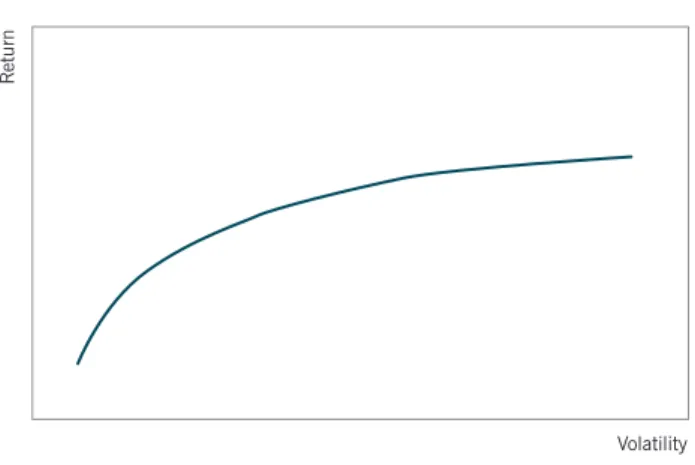
Most traditional asset allocation models follow some variant of mean variance optimization, pioneered by Harry Markowitz in the 1950s.3 Mean varianceoptimization characterizes assets according to their expected return, volatility, and correlation to one another.4 Based on these estimates, as well as an
investor’s risk target, mean variance optimization creates an “efficient frontier,” which identifies portfolios that produce the highest level of return for a given level of risk (as Display 1 illustrates).3
Display 1:
Illustration of Mean Variance Optimization Approach
2 Note that this paper focuses on risks generated by underlying
investments, not on the larger set of risks that an investor faces. For example, it does not consider the risk of underperforming peers. While these risks are important, they fall beyond the scope of the paper.
R
eturn
Volatility
3 Source: Markowitz, H.M. Portfolio Selection. The Journal of Finance.
March 1952.
4 “Expected return” is an estimate of an investment’s average future
return. “Volatility” is the degree of movement around the average return. “Correlation” is the degree to which the returns of different investments move together.
Mean variance optimization has been well studied, and is relatively easy to implement. However, this technique rests on two implicit assumptions that do not hold in practice. First, it assumes comparability across asset classes. In other words, mean variance optimization uses the same techniques to model the risk and return of equities as it does for private equity and hedge funds. Unfortunately, each of these asset classes consists of different types of returns, with very different associated risks. treating asset classes in a similar fashion tends to mischaracterize (and potentially understate) the risks that investors face. Second, it makes decisions myopically, without considering how the portfolio (or an investor’s needs) may evolve in the future. If an investor’s needs are stable, and the portfolio is fully liquid, this approach leads to reasonable solutions. If, however, investor needs vary over time or if today’s decisions limit an investor’s future options, a myopic approach leads to portfolios that may fail investors at particular points in time.
While these assumptions may have been reasonable in a world of stocks, bonds, and cash, they fail to capture the complexities of current investments such as emerging market equity, hedge funds, and private real estate.5 The
remainder of this section examines each limitation in more detail.
Accounting for Multiple Sources of Return
traditional asset allocation treats all asset classes in the same fashion. It compares assets based on their expected return, volatility, and correlations. These comparisons may work across stocks, bonds, and cash, but break down when considering a larger set of investment choices. The reason is that certain investment choices have a very different risk and return profile than others. For example, consider three investments: a U.S. large cap equity etF, a U.S. large cap equity manager, and a private equity manager. The returns from the first investment depend directly on the performance of U.S. equity markets. Performance of the second investment depends primarily on the performance of U.S. equity, but also on the investment manager’s investment acumen. Finally, the performance of a private equity fund depends on three factors: U.S. equity market performance, the investment manager’s acumen, and the liquidity premium generated from investing in less liquid assets. treating these three investments in the same fashion ignores the fact that each investment generates returns in different ways, and entails very different types of risks. Investors need a way to properly account for the risks embedded in each investment when making portfolio decisions. One option is to separately model the risk characteristics investment by investment. In practice, however, the large number of investments in most portfolios prohibits this approach. a second option, which aIP advocates, is to focus on the underlying drivers of risk and return within each asset class. While the specific characteristics of each investment option may differ significantly, all investments generate returns from one of three sources: beta, alpha, and liquidity (illustrated in Display 2).
5 Even in the traditional world of stocks, bonds, and cash, mean
variance optimization does suffer some limitations. In particular, the recommended allocations are very sensitive to the input assumptions, meaning that small changes in return forecasts could have a large impact on portfolio allocations.
Display 2:
Sources of Return
Beta refers to returns driven by fundamental
macroeconomic factors such as gDP growth, interest rates, and inflation. These returns correspond to the returns of major asset classes, such as U.S. equity, high yield, and commodities. Since the global economy has grown over the long run, and beta returns depend on macroeconomic performance, beta has historically delivered positive returns on average.
Alpha refers to skill-based returns. These are returns generated by a manager’s active decisions regarding market timing or security selection. Since each manager generates a unique alpha, investors can choose from a virtually infinite number of alphas. Unlike beta, alpha is a zero-sum game. The excess returns that one investor generates through successful stock picking or market timing comes at the expense of another investor. a well diversified portfolio of alphas will not necessarily generate positive returns, and could produce negative performance.
Liquidity refers to the returns investors generate for investing in non-traded assets. For example, investors allocating to private equity typically cannot access their capital for a multi-year period. In exchange for giving up the option to sell their position, investors expect to earn
a higher rate of return over time. Like any option, the liquidity premium depends on the horizon (i.e., lockup period) and on the volatility of the underlying asset class. Therefore the liquidity premium will differ across
6 Skew refers to the asymmetry of a return distribution, or the extent
to which it leans to one side. Kurtosis refers to the peakedness of a
probability distribution. Distributions with significant kurtosis have
a greater chance of producing abnormally large or small outcomes relative to normal distributions. Note that skew and kurtosis are often discussed in reference to downside risk, but can also increase upside potential. For example, some private equity strategies are particularly attractive over time because of positive skew.
7 Source data: historical hedge fund manager data from PerTrac; private equity returns from Venture Economics; index returns from
Bloomberg which include MSCI Emerging Markets Index, S&P 500, CSFB Leveraged Loan Index, Barclays Aggregate Bond Index, and Merrill Lynch Convertible Index. Data covers 1990 through 2008.
Risks Associated with Each Source Return
Traditional approaches only focus on one form of risk: volatility. Volatility appropriately captures risk if returns follow a normal distribution. Unfortunately, if investment returns follow non-normal distributions,
volatility may significantly understate downside risk.
AIP uses measures of skew and kurtosis, in addition to volatility, to capture the non-normal aspects of an investment’s return distribution.6
Since the risk of an investment depends on its sources of return, AIP directly models the volatility, skew, and kurtosis of each return source, and then aggregates these at the investment level. Table 1
below illustrates the distributional characteristics of each return source:
Table 1:
Distributional Characteristics of Each Return Source7
Importance as a Driver of Risk
Volatility Skew Kurtosis
Beta High Moderate Moderate
Alpha High Low Low
Liquidity High High High
Return
Liquidity Beta
Alpha
• Asset class returns
• Driven by fundamental factors (e.g., GDP growth)
• Returns from manager skill
• Usually based on security selection or market timing
• Premium associated with holding liquid investments
5
asset classes (e.g., one would expect a greater liquidity premium in private equity than in private real estate, since private real estate typically has lower volatility than, and returns cash more quickly than, private equity). These differences lead to highly varying risk profiles across each return source. Investing in illiquid assets entails significant downside risk, since these assets may rapidly lose value during liquidity shocks. additionally, investing in active managers entails significant forecast risk (i.e., risk that one’s forecasts are incorrect) since the long run performance of alpha has been much less certain than the long run performance of beta. as one example, the callout box describes how aIP accounts for differences in return distributions for alpha, beta, and liquidity. each investment option generates returns from some combination of beta, alpha, and liquidity. Display 3
illustrates this point in more detail.
as indicated in Display 3, an equity etF generates all of its return from beta. By contrast, a distressed hedge fund manager generates some return from beta, some from alpha, and some from liquidity. Understanding the sources
of return embedded in each investment may help investors better understand the associated risks and may enable them to make more intelligent portfolio allocation decisions. Instead of making allocation decisions across asset classes, aIP recommends that investors allocate across sources of return, as Display 4 illustrates. This provides a more transparent view of portfolio risk, and helps ensure that an investor’s portfolio matches the investor’s risk profile.
Display 4:
Comparison of Traditional Asset Allocation and a New Approach to Asset Allocation9
Traditional Model New Approach
Display 3:
Sources of Return for Sample Investments8
Equity ETF
Distressed HF Equity Market Neutral HF
Active Long–Equity
Beta Alpha Liquidity
Equity 40% Hedge
Funds 15%
Fixed Income 30%
Private Real Estate 5% Private
Equity 10%
Alpha 20%
Equity 40% Hedge
Funds 15%
Fixed Income 30%
Private Real Estate 5% Private
Equity 10%
Beta 60% Alpha
20%
Liquidity 20%
8 Source: AIP 9 Source: Examples of the traditional approach can be found in Secrets
of the Academy: The Drivers of University Endowment Success, Harvard Business School Finance Working Paper, October 2007.
Accounting for Portfolio Evolution
In addition to focusing on asset classes, traditional asset allocation is myopic. It makes decisions based on conditions today, without considering how those conditions may change going forward. This type of an approach ignores three important factors:
1. Asset class characteristics change significantly over time – although risk and return characteristics of many investments have been stable over very long periods, they may change significantly in the short to medium term. For example, the S&P 500 volatility fell to 10% during 2007, and then spiked to well over 50% during the second half of 2008.10 This created large losses for
many investors who over-allocated to equity assuming that volatility would remain constant. additionally, the average returns of asset classes may vary
significantly across market cycles. as Display 5
indicates, the 10-year return for U.S. equity was less than 5% for most of the 1960s, but above 10% throughout the 1980s and early 1990s.
2. Decisions made today may affect investors’ future options – Investors who allocate to illiquid asset classes lose the ability to change these allocations in the future (at least for a several year period). This causes the actual portfolio weights to drift away from an investor’s desired allocation.
3. Investors’ needs vary with time – Investors’ financial needs, such as cash flow requirements, may vary significantly over time. In addition, these needs may correlate with portfolio performance. For example, periods of market stress may limit an endowment’s ability to raise money from alumni, and simultaneously lead to losses in the investment portfolio. traditional optimization has no ability to account for these changes when choosing a portfolio.
-10 -5 0 5 10 15 20%
1950 1952 1954 1956 1958 1960 1962 1964 1966 1968 1970 1972 1974 1976 1978 1980 1982 1984 1986 1988 1990 1992 1994 1996 1998
Display 5:
Annualized 10 year S&P 500 Returns (Measured Over Subsequent Years)11
11 Source: Underlying S&P 500 total return data obtained from
Bloomberg. Computation of 10-year forward returns performed by AIP. 10-year returns illustrated in Display 5 span January 1950 through July 1999 timeframe. Past performance is not indicative of future results.
10 Source: Based on VIX index, which measures the implied volatility
of the S&P 500 index. Implied volatility refers to the volatility level embedded in options prices, and measures investors’ collective view on future volatility. VIX data obtained from Bloomberg.
aIP’s Portfolio Construction approach
aIP has designed a new framework that seeks to overcome the limitations of traditional asset allocation models. The framework extends the traditional asset allocation approach in two dimensions: across source of return, and across time.Extensions across source of return – Instead of assuming that all asset classes behave in the same way as equity and fixed income, our framework recognizes that each investment consists of a unique combination of alpha, beta, and liquidity. When making portfolio decisions, aIP decomposes investments across these three return sources and chooses allocations across return sources instead of across asset classes.
Extensions across time – Our framework accounts for a portfolio’s evolution over time. It models the characteristics of each return source over time, to capture changes in the risks, returns, and correlations across investments. It then considers these potential changes as well as an investor’s needs over multiple periods when choosing an optimal portfolio. This approach may help avoid portfolios that provide attractive average characteristics, but may deviate from these characteristics significantly during any given period.
Like traditional optimization, aIP starts with the three-stage process of 1) understanding historical performance, 2) generating risk and return forecasts, and 3) running an optimization to seek to identify portfolios that best suit an investor’s needs. However, our implementation differs significantly from traditional approaches. aIP applies this process across sources of return, as opposed to traditional optimization, which focuses on total return. aIP then extends each of these stages across time.
Display 6 illustrates the process, and provides a brief
description of each stage.
Display 6:
AIP Asset Allocation Framework
aIP starts by disaggregating returns for each investment into beta, alpha, and liquidity components, and tracking how these components have changed historically. For example, this allows one to estimate a long/short equity manager’s historical exposure to the S&P 500, as well as track how that exposure changed over time.
aIP then generates forecasts for the average behavior of each return component, and project how these components are likely to evolve around their average. Consider a manager with an average net exposure of 0.5 historically, but whose beta varied significantly around that average. aIP may forecast a future average beta of 0.5, but also simulate deviations around the average. Our forecasts consider the possibility that in any given future period, the manager’s actual beta may be significantly higher or lower than the manager’s average beta.
Similar to traditional optimization, our approach chooses a portfolio that seeks to best match an investor’s preferences. However, the optimization stage of our approach differs from that of traditional optimization in two ways. First, it incorporates different forms of risk. For example, investors face significant forecast risk when allocating to active
Disaggregation
Forecasting
Optimization
First Dimension: Across Return Source Splits historical returns for each investment into alpha, beta, and liquidity components Projects average risk and return characteristics of each return source Incorporates multiple forms of risk into allocation decision
Second Dimension: Across Time
Tracks changes in these components over time Simulates how these characteristics may evolve going forward Chooses allocation based on changes in investor needs over time, and changes in investment characteristics over time
managers. Since alpha generation is highly uncertain, investors face substantial risk that their alpha forecasts are incorrect. aIP accounts for these types of risks when building portfolios.12 Second, instead of building a
portfolio that matches an investor’s current needs with the current characteristics of various investments, it chooses a portfolio based on the evolution of an investor’s needs over time, and the evolution of investment characteristics over time. This may lead to portfolios that perform well over an investor’s entire investment horizon.
The remainder of this section illustrates our framework using a series of examples.
Return Disaggregation (Across Return Source)
Return disaggregation involves separating an investment’s returns into the three sources described earlier: beta, alpha, and liquidity. to better understand this process, consider a mutual fund manager benchmarked against the S&P 500. Movements in the S&P 500 will explain most of this manager’s performance. However, the manager’s decisions regarding which stocks to overweight or underweight will also influence performance. These decisions collectively represent a manager’s alpha, which is uncorrelated with the beta component of return. Historically, investors have defined alpha as the excess of a manager’s return relative to a benchmark. For example, if the manager generates a 10% return, and the S&P 500 generates a 9% return during the same period, investors would attribute 100 bps of alpha to the manager. This approach, however, fails to distinguish how the manager generated a 10% return. Consider two managers, a and B, as Display 7 illustrates.13
Display 7:
Comparison of Two Long Only Equity Managers
Historical Performance of Two Large Cap Managers: Illustrative Example
Manager A Manager B
Total Return 17.6% 16.4%
Volatility 22.0% 21.6%
Standard Alpha 6.1% 4.9%
Beta 1.5 1.0
Skill Based Alpha 0.4% 4.9%
as indicated, Manager a outperforms B based on the conventional measures of alpha: between 1990 and 2009, this manager outperformed the benchmark by 6.1%, as compared to 4.9% for Manager B. Unfortunately, this type of analysis ignores how each manager
outperformed the benchmark. a closer inspection reveals that Manager a’s performance correlates very highly with benchmark performance. Manager a outperforms when the benchmark delivers strong performance, and underperforms when the benchmark delivers negative performance. effectively, Manager a’s outperformance comes from additional market risk, which investors could easily obtain on their own. This form of outperformance does not create any value for investors.
80% 60 40 20 0 -20 -40
1990 1992 1994 1996 1998 2000 2002 2004
Manager A Manager B
12 Due to various uncertainties regarding risks, AIP makes no guarantee
of being able to account for all risks for all portfolios.
13 Example is purely hypothetical. It does not reflect the performance of
any Morgan Stanley investment.
Manager B, by contrast, produces a very different return profile. While the benchmark explains some of Manager B’s returns, a component also comes from the manager’s unique decisions. For example, during early 2000, Manager B generated positive returns, while the benchmark produced negative returns. The excess performance that Manager B generates comes from investment skill, not from additional market risk. Properly evaluating these managers requires an approach that accurately separates manager skill from market exposure. One way to accomplish this is through a statistical technique known as regression. Regression compares the pattern of a manager’s return to that of multiple factors, and extracts the component of return corresponding to market factors. The residual return is
uncorrelated with the market returns, and represents a
manager’s alpha. Display 8 illustrates this process through a simple example.
Display 8:
Measuring the Alpha of a Long Only Equity Manager14
The above plots a manager’s return (excess of cash) relative to the S&P 500 return (also excess of cash). The slope of the line indicates the manager’s beta, which in this example is 0.5. It shows that on average, the manager’s return increases by 50 bps for every 1% increase in the S&P 500. The intercept indicates the manager’s alpha, or the component of the manager’s return that is uncorrelated with the benchmark. Finally, the dispersion around the line indicates the volatility of the manager’s alpha (which is also known as active risk). It shows how much risk a manager expends in generating alpha.
Isolating manager alpha helps enable investors to make fair comparisons across different types of managers. Comparing the total returns of a long short equity manager and long only mutual fund manager does not make sense, since the former will typically have much less market exposure than the latter. Comparing one manager’s alpha to another, however, may help investors identify which manager is more skilled.15 Furthermore,
if investors can measure the amount of alpha and beta within each manager, they can properly account for the risks of each when building portfolios.
Return Disaggregation (Across Time)
The above approach assumes that a manager’s exposure to market factors is constant. However, many managers (particularly hedge fund managers) vary their market exposures significantly over time. This variation could stem from market timing decisions, or could simply be a byproduct of their stock picking. In either case, standard factor models cannot capture these variations.
0 5 10 15 25% 20
5 10 15%
Active Risk
Alpha
Beta
14 The above information is purely hypothetical and for illustrative
purposes only and does not represent the performance of any
specific investment.
15 In addition to evaluating managers based on their alpha, AIP
compares them based on information ratio, which is the ratio of a manager’s alpha to the manager’s alpha volatility (the degree that a manager’s alpha varies around its average value). This is a better measure of skill than alpha alone, since it measures how much alpha a manager generates per unit of risk (in other words, how
aIP has addressed this challenge through developing dynamic factor models. Instead of assuming constant levels of market exposure, these factor models allow for variations in market exposure over time. Display 9 illustrates the results of applying a dynamic factor model to a long short equity manager. as indicated, the manager’s exposure to U.S. equity varies from a low of zero to a high of almost two. Identifying these changes is critical to accurately measuring portfolio risk, since both the manager’s volatility, and correlation to the equity markets, depends on levels of market exposure.
Display 9:
Estimate of Equity Long/Short Manager’s Beta Over Time16
Exposure of Equity Long/Short Manager Relative to S&P 500
In addition to bolstering risk management, capturing changes in beta over time may allow investors to quantify a manager’s market timing ability. Market timing decisions correspond to increases or decreases in market exposure relative to the average level of market exposure. If a manager increases beta exposure as markets are rising, and reduces exposure as markets are falling, he will generate positive returns from market timing. By quantifying the changes in a manager’s market exposure
around its average level, dynamic factor models may enable investors to estimate market timing returns.17
as an example, Table 2 decomposes the equity long/short manager’s returns into three components: average beta, market timing, and security selection. as indicated, the manager generates value through both security selection and market timing. This information can help determine the appropriate role of the manager within a broader portfolio, and better evaluate manager performance over time.
Table 2:
Return Disaggregation for Long/Short Hedge Fund Manager18
Return Risk Return/Risk
Security Selection Alpha 2.70% 8.30% 0.32
Market Timing Alpha 2.20% 7.40% 0.30
Average Beta -2.70% 10.00% (0.27)
Total 5.10% 13.50% 0.16
Importantly, investors should recognize that statistical estimates of alpha and beta are only approximations, and should be used in conjunction with an investor’s qualitative understanding of a manager’s strategy. For example, a regression model may show that a hedge fund has very strong alpha generation ability. If, however, an investor knows that several key analysts recently left the hedge fund, he may question whether the fund’s alpha generation ability is sustainable. Under this scenario, the investor’s qualitative knowledge of the hedge fund may be more important than the regression model results.
16 Source: Return data for long/short equity manager obtained from
PerTrac. Beta estimates based on proprietary dynamic factor model. For illustration only. Not indicative of expected return of any portfolio.
1/08 1/09 -0.5
0 0.5 1.0 1.5 2.0
1/02 1/03 1/04 1/05 1/06 1/07 Average Beta
Actual Beta
17 The dynamic factor models are implemented using a Kalman filtering
approach, which generates estimates of a manager’s beta(s) at each point in time. See Kalman, R.E., “A New Approach to Linear Filtering and Prediction Problems” in JOURNAL OF BASIC ENGINEERING, No. 82, 1960.
18 Source: Return data obtained from Pertrac. Disaggregation based
on proprietary return attribution models. For illustration only. Not indicative of future performance of any strategy or manager.
Forecasting – Across Return Source
traditional optimization forecasts performance using historical data. The problem with this approach is that historical data provide an uncertain estimate of future performance. For example, consider two investments that both provide the same average return. During any given period, one investment will outperform the other purely by chance. as a result, traditional optimization techniques favor investments that have performed best historically, even if the outperformance occurred purely by
chance. as a result, they allocate too much to investments
that have performed well historically, and too little to the investments that have performed poorly, leading to an unbalanced portfolio.
although historical data suffer from limitations, it does provide some information regarding future outcomes. For example, most investors would expect equities to outperform fixed income going forward, since this relationship has held true historically. The challenge, therefore, is combining historical data with other information in a way that produces reasonable forecasts. Our approach relies on a technique known as “Bayesian Forecasting.” This process allows investors to specify views regarding an investment’s future returns, as well as a confidence level in those views. It then statistically combines these views with historical data to produce a consistent set of forecasts across all investment options. This technique applies to any source of return; for illustrative purposes, however, aIP shows how to apply this technique to forecasting a manager’s alpha. Consider a global macro manager who has historically generated 2% alpha. Using the historical data only, our best estimate of this manager’s future alpha would also be 2%. However, since we have limited data (in this example, a 3 year track record) there is significant uncertainty around this 2% estimate. Display 10 shows the forecast and associated uncertainty.
Display 10:
Estimated Historical Alpha, and Uncertainty Surrounding Estimate19
In addition to the historical data, investors may hold certain beliefs regarding this manager’s ability. For example, they may know of other managers who follow similar strategies, and have generated a 10% alpha. absent any historical data regarding this particular manager, one may assume that this manager will also generate a 10% alpha. However, like the historical data, this 10% simply represents an estimate, and contains significant uncertainty.
aIP can develop a forecast by statistically combining these two sources of information, as Display 11 illustrates. The final forecast is a weighted average of the 2%
historical estimate, and 10% prior estimate, where the weights depend on the uncertainty in each estimate. For example, if we are highly confident about the historical performance (e.g., the manager has an exceptionally long track record) we may weight the 10% estimate more heavily than the 2% estimate. In this example, we give more weight to the prior view, since the manager has a relatively short track record.
Estimate Uncertainty
2% Estimated Alpha
19 The above information is purely hypothetical and for illustrative
purposes only and does not represent the performance of any
Display 11:
Example of Bayesian Forecasting Process19
Optimization – Across Return Source
as described earlier, each return source creates different types of risks, which investors must recognize when choosing portfolios. Focusing solely on volatility, however, ignores a number of these risks. For example, one of the most significant risks that investors face, particularly when investing in alpha, is estimation error, or the risk that forecasts are wrong. The previous section alluded to this risk, noting that all forecasts are inherently uncertain. In other words, aIP may believe that U.S. equity will deliver long-term returns of 8%, but actual long term returns could differ significantly from our estimates. Unfortunately, traditional optimization ignores this risk when building portfolios. Mean variance optimization assumes that an investor’s forecasts are correct, and builds a portfolio that performs well given an
investor’s forecasts. However, if actual performance deviates
significantly from projections, the portfolio may not perform as expected.
to better understand this point, revisit the forecasting example in Display 11. aIP expects that the manager will generate a 7% alpha on average, but the forecast contains significant uncertainty. The true average alpha (which is unobservable) could fall anywhere within the center distribution. This uncertainty regarding the average return creates additional risk for investors.
Display 12 compares the distribution of future returns
for a manager with a projected 5% alpha, and 0.75 beta, under two scenarios: a) the forecasts exactly match reality (as traditional optimization assumes) and b) the forecasts contain uncertainty. as indicated, estimation error widens the distribution of future returns. The wider distribution recognizes that the actual alpha could prove lower than expected, and the actual beta may be higher than expected, both of which increase the probability of loss.
Display 12:
Return Distribution With and Without Forecast Risk20
aIP believes that investors should directly account for forecast risk when building portfolios. Our approach is to quantify each investment’s estimation error, and simulate a range of possible returns and beta exposures. We then seek to choose portfolios that may perform well across all scenarios.
-12% -8% -4% -0% -4% -8% -12% -16% -20% -24% No Estimation Error
Estimation Error
20 The above information is purely hypothetical and for illustrative
purposes only and does not represent the performance of any
specific investment. Historical Alpha = 2%
3 Years of Data
Prior Alpha = 10% 5 Year Confidence Projected Alpha = 7%
Optimization – Across Time
In most cases, portfolio strategy involves decision making over multiple periods. For example, investors allocating to private equity cannot simply buy an existing private equity investment.21 Rather, they periodically commit
capital to private equity funds, and gain exposure to private equity as they fund capital calls. Similarly, investors periodically rebalance their portfolios. The rebalancing frequency depends on transactions costs, and the liquidity of the underlying investments. In both scenarios, investors need to make investment decisions over time. Moreover, the decisions made in current periods may constrain an investor’s future options. Overcommitments to private equity, for
example, may lead to very high private equity allocations. This could limit an investor’s ability to rebalance the portfolio, meet future cash flow needs, or take advantage of new (and potentially better) investment opportunities in the future.
For this reason, investors need a framework that accounts for decision making over the entire investment horizon. They need to understand the cost of today’s decisions in future periods, and account for this cost when constructing a portfolio.
aIP addresses this challenge through a multi-period optimization that explicitly considers the future costs of an investor’s current decisions. as an example, consider the challenge of designing a private equity commitment strategy. One simple approach has been to hold the investments, plus unfunded commitments,22
constant. Following such a strategy (assuming a target 20% allocation) produces the allocation profile shown
in Display 13 (dark green line). as indicated, such a
strategy produces significant fluctuations in private equity allocations. During early periods, investors are underallocated to private equity, and increase
commitments. eventually these commitments are drawn, leading to an overinvestment in private equity. Investors then cut back on private equity commitments, leading to an underinvestment in private equity. The allocations eventually stop oscillating, but require 20 years to stabilize. The overshoots and undershoots are caused by a myopic investment strategy.
The investor bases today’s commitment decision on today’s allocation and unfunded commitments, without considering the likely impact of these decisions (and previous decisions) in the future.
Display 13:
Comparison of Commitment Strategies23
By incorporating their knowledge of the future into today’s decisions, though, investors may realize better outcomes. Consider a strategy that bases commitments today not just on current private equity investment levels, but on expected future investment levels. The light green
0 Yr 15 Yr 14 Yr 13 Yr 12 Yr 11 Yr 10 Yr 9 Yr 8 Yr 7 Yr 6 Yr 5 Yr 4 Yr 3 Yr 2 Yr 1 2 4 6 8 10 12 14
—Strategy 1 —Strategy 2
Projected Private Equity Allocation
Allocation
23 The above information is purely hypothetical and for illustrative
purposes only and does not represent the performance of any
specific investment. 21 Technically, investors could access private equity investments
through a secondary market. However, the attractiveness and
depth of this market varies significantly over time, and investors
cannot permanently rely on the secondary market as an attractive source of liquidity.
22 Unfunded commitments are commitments that have been made but
line in Display 13 shows the allocations of such a strategy over time, which aIP developed using a proprietary multi-period allocation model. While reaching the target allocation takes more time, the allocation profile is more stable. In early periods, this strategy will recognize that capital calls are likely to increase, and therefore will not commit as much as the first strategy. although the steady state characteristics of both strategies are the same (i.e., both reach target allocations of 20%) most investors would prefer the second strategy as it leads to less volatility along the way.24
For investors, the critical question is whether the aIP approach outperforms traditional asset allocation. We believe that our framework helps investors in a number of ways.
First, the attribution tools seek to help investors better understand which managers are adding value, and how that value is being created (i.e., through market timing or security selection). This can help investors filter managers who add little value, and allows investors to compare managers with very different investment styles.
Second, by making allocation decisions across return
sources, aIP’s framework can build a portfolio that seeks to match investor preferences across multiple forms of risk. For example, our approach can potentially limit the amount of forecast risk, or downside risk, within a portfolio.
Third, aIP’s approach seeks to account for changes in
both investor needs and investment characteristics when building portfolios. traditional optimization, by contrast, assumes that investor needs and investment characteristics are fixed.
Display 14:
Comparison of Cumulative Performance of Two Managers (Assuming $100 Starting Capital)25 450
400 350 300 250 200 150 100 50 0
5/02 9/02 1/03 5/03 9/03 1/04 5/04 9/04 1/05 5/05 9/05 1/06 5/06 9/06 1/07 5/07 9/07 Emerging Market
Manager
Market Neutral Manager
24 When structuring a private equity program, investors should also focus on obtaining diversification across geographies and vintage
years. Further, private equity consists of many underlying asset classes, such as venture capital, U.S. leveraged buyouts, and
international buyouts. Investors should maintain diversification
across these underlying asset classes as well.
25 Source: Return data for long/short equity manager obtained from
PerTrac. Beta estimates based on proprietary dynamic factor model. For illustration only. Not indicative of expected return or performance of any strategy or manager. Data for chart spans January 2002 through December 2007 timeframe. Past performance is not indicative of future results.
Table 3:
Manager Return Attribution27
Emerging Market Manager Market Neutral Manager
Return Risk Return/Risk Return Risk Return/Risk
Alpha 1.40% 7.20% 0.19 5.50% 3.70% 1.48
Beta 21.20% 15.10% 1.41 1.50% 4.20% 0.36
Total (excl. cash) 22.60% 18.30% 1.24 7.00% 5.80% 1.20
However, investors should remember that all asset allocation approaches (including aIP’s) are simplifications of reality. While aIP believes that our approach does a much better job capturing actual investment risks than traditional portfolio construction techniques, it will never capture every risk that an investor faces. For example, accurately modeling the risk of private equity and private real estate is extremely difficult since these assets are infrequently marked to market.26 Therefore,
supplementing our approach with experience and judgment is critical. In addition, during periods such as 2008, the vast majority of investments can
simultaneously deliver poor performance. aIP’s approach by no means can prevent significant losses during these periods. Rather, our tools should provide investors a more robust understanding of the risks that they face, and an ability to choose a portfolio that can help meet their investment objectives.
In this spirit, aIP presents two examples of our asset allocation framework, both comparing our results to those of more traditional approaches.
Evaluating Hedge Fund Manager Performance as previously described, evaluating hedge funds using traditional metrics alone can be highly misleading, since hedge funds have very different return profiles. Properly evaluating hedge funds requires isolating each manager’s alpha. Unless investors separate alpha from total return, they risk selecting managers based on their market returns, as opposed to selecting managers based on investment skill. as an example consider two equity managers: an emerging market long short equity fund, and a U.S. equity market neutral fund. Display 14
illustrates the performance of each fund from January 2002 through December 2007.
From a total return standpoint, the emerging market manager clearly outperformed over the period, returning 25.7% as compared to 10.1% for the market neutral manager. On a risk-adjusted basis the two managers performed more comparably, but the emerging market manager delivered slightly better performance, yielding a 1.24 Sharpe ratio, compared to the market-neutral manager’s 1.20 Sharpe ratio. Investors who evaluated these managers on a total return basis would likely have selected the emerging market manager over the market neutral manager.
26 Certain modeling techniques do exist for generating better estimates of
private equity and private real estate risks. For example, see How Risky are Illiquid Investments? Budhraja, Vineet and de Figueiredo, Rui. Journal of Portfolio Management. Winter 2005. However, even these techniques are only approximations of reality, and the resulting risk estimates are less accurate than those of more liquid asset classes.
27 Source: Return data obtained from PerTrac. Disaggregation
based on proprietary return attribution models. For illustration only. Not indicative of expected return or performance of any manager or strategy.
Designing a Strategic Portfolio
as discussed in Section 1, traditional optimization does not account for the cost of today’s decisions in future periods. If investors are allocating to liquid assets, this cost may be minimal, because they can always change their portfolio in the future. However, when allocating to illiquid assets such as private equity, private real estate, and certain hedge fund strategies, these costs could become substantial. For example, investors with large illiquid allocations cannot easily rebalance their portfolios, face difficulty in capitalizing on new investment opportunities, and may struggle to meet unforeseen cash flow requirements. This raises two issues for investors when designing portfolios. First, traditional optimization does not account for these costs, and therefore may allocate too much to illiquid assets. Second, these costs are a function of how effectively one implements allocations to illiquid assets — the better cash flows from these assets are managed, the lower these costs. as an example, consider an investor who is invested in traditional equity and fixed income assets and adds an allocation to private equity. This investor has a moderate risk profile, and is willing to accept a fair amount of illiquidity, but also wants to preserve capital. aIP constructed two portfolios for this hypothetical investor based on estimated characteristics of the various asset categories: one (the “static model”) which uses a rule that statically allocates (or commits) to private equity, and one (“dynamic model”) which dynamically optimizes allocations to private equity based on actual cash flows. However, comparing these managers based on their
alpha characteristics yields a very different picture.
Table 3 provides the return attribution for each manager.
as indicated, the emerging market manager generated the majority of his returns from emerging market equity exposure, as opposed to alpha. By contrast, the market neutral manager generated the bulk of returns from security selection, and very little came from market exposure. Further, the market neutral manager generated alpha much more efficiently per unit of risk; his information ratio was 1.5, versus 0.2 for the emerging market manager.
The difference between these managers became apparent during 2008. as equity markets around the world collapsed, the emerging market equity manager suffered a 50% loss. By contrast, the market neutral manager, whose performance depends much more heavily on security selection, only lost 7%. Investors who did not understand the contribution of alpha versus beta to each manager’s total return may have over allocated to the emerging market equity manager, and ended up with excess beta risk.
Display 15 shows the expected allocations after three years in each of these cases.28Display 16 shows a measure
of expected risk-adjusted performance of the static and the dynamic approaches in the first three years, based on our illustrative risk and return calculations. It compares these to a benchmark case of a portfolio optimized only with traditional equity and fixed income.29
Display 15:
Comparison of Strategic Portfolios30
Based on these results, two important conclusions about the various approaches are apparent. First, by optimizing allocations to private equity, an investor may be able to reduce the “cost” of illiquidity significantly. This is apparent in Display 15: allocations under the dynamic approach are higher than in the static case because the dynamic case better manages portfolio liquidity. typically, portfolios with illiquid assets will drift away from their
Private Equity
Equity Fixed Income
24.6%
16.6%
58.8% 20.7%
26.9%
52.3%
Static Dynamic
28 In this example, AIP uses a finite horizon of three years. 29 For simplicity, risk-adjusted performance is measured as the
expected excess-to-cash return minus a risk-aversion coefficient multiplied by the portfolio variance. The figure shows an index in
which the risk-adjusted performance of the portfolio of equity and
fixed income only is normalized to one.
30 The above information is purely hypothetical and for illustrative
purposes only and does not represent the performance of any
specific investment.
target allocations over time as investors cannot easily rebalance the illiquid positions. Since the dynamic approach considers the impact of today’s decisions over multiple periods, it better accounts for portfolio drift, thereby reducing the cost of investing in private equity. This effect can be seen by examining the expected performance in Display 16: the static approach generates systematically lower risk-adjusted returns when compared to an approach which appropriately optimizes the allocations over time.
Display 16:
Illustrative Comparison of Dynamic and Static Approaches31
Expected Risk-Adjusted Performance
Second, the value of allocating to the illiquid asset class is potentially significant. In Display 16, even with the illiquidity of private equity, the investor’s risk-adjusted performance is higher by including a broader range of asset categories than when the investor is constrained to allocate to only fixed income and equity.
31 The above information is purely hypothetical and for illustrative
purposes only and does not represent the performance of any
specific investment. 0.95
1.00 1.05 1.10 1.15 1.20
Year 1 Year 2 Year 3
1.25
Dynamic
Static
Conclusion
traditional asset allocation approaches rest on two key assumptions: volatility and correlations properly account for risk across all asset classes, and portfolio characteristics (as well as investor needs) remain constant over time. These assumptions unfortunately do not hold in practice, and lead to particularly poor decisions when allocating to sub-asset classes, active managers, and alternative investments. Recognizing these limitations, aIP has developed a new asset allocation framework that extends traditional portfolio optimization in two ways: across sources of return, and across time. aIP recognizes that investment risks differ significantly by source of return (beta, alpha, and liquidity) and therefore structures portfolios around return sources instead of around asset classes. Further, we recognize that portfolios evolve over time, and account for these changes when building portfolios. This may lead to solutions that match investor requirements over their entire investment horizon.
The performance of any portfolio strategy depends heavily on the performance of underlying investment choices, and aIP’s approach is no exception. For example, our approach would not have circumvented the problems that investors faced during 2008. That said, aIP’s asset allocation framework may provide investors a better understanding of the investment risks they are taking, and may help investors choose portfolios that meet their long-term goals.
Past performance is not indicative of nor does it guarantee comparable future results.
This piece has been prepared solely for informational purposes and is not an offer, or a solicitation of an offer, to buy or sell any security or instrument or to participate in any trading strategy.
Alternative investments are speculative and include a high degree of risk. Investors could lose all or a substantial amount of their investment. Alternative instruments are suitable only for long-term investors willing to forego
liquidity and put capital at risk for an indefinite period of
time. Alternative investments are typically highly illiquid-there is no secondary market for private funds, and there may be restrictions on redemptions or assigning or otherwise transferring investments into private funds. Alternative investment funds often engage in leverage and other speculative practices that may increase volatility and risk of loss. Alternative investments typically have higher fees and expenses than other investment vehicles, and such fees and expenses will lower returns achieved by investors.
Alternative investment funds are often unregulated and are not subject to the same regulatory requirements as mutual funds, and are not required to provide periodic pricing or valuation information to investors. The investment strategies described in the preceding pages
may not be suitable for your specific circumstances;
accordingly, you should consult your own tax, legal or other advisors, at both the outset of any transaction and on an ongoing basis, to determine such suitability.
AIP does not render advice on tax accounting matters to clients. This material was not intended or written to be used, and it cannot be used with any taxpayer, for the purpose of avoiding penalties which may be imposed on the taxpayer under U.S. federal tax laws. Federal and state tax laws are complex and constantly changing. Clients should always consult with a legal or tax advisor for information concerning their individual situation.
The information contained herein may not be reproduced or distributed.
This communication is only intended for and will only be distributed to persons resident in jurisdictions where such
Morgan Stanley is a full-service securities firm engaged
in securities trading and brokerage activities, investment
banking, research and analysis, financing and financial
professional services.
The views expressed herein are those of Alternative lnvestment Partners (“AIP”), a division of Morgan Stanley Investment Management, and are subject to change at any time due to changes in market and economic conditions. The views and opinions expressed herein are based on matters as they exist as of the date of preparation of this piece and not as of any future date,
and will not be updated or otherwise revised to reflect
information that subsequently becomes available or circumstances existing, or changes occurring, after the date hereof. The data used has been obtained from sources generally believed to be reliable. No representation is made as to its accuracy.
An investor cannot invest directly in an index, and
performance of an index does not reflect reductions for
fees and expenses. Past performance is no indication of future performance.
Information regarding expected market returns and market outlooks is based on the research, analysis, and opinions of the investment team of AIP. These conclusions are speculative in nature, may not come to pass, and are not intended to predict the future of any
specific AIP investment.
The information contained herein has not been prepared in accordance with legal requirements designed to promote the independence of investment research and is not subject to any prohibition on dealing ahead of the dissemination of investment research.
Certain information contained herein constitutes
forward-looking statements, which can be identified by the use
of forward looking terminology such as “may,” “will,” “should,” “expect,” “anticipate,” “project,” “estimate,” “intend,” “continue” or “believe” or the negatives thereof or other variations thereon or other comparable terminology. Due to various risks and uncertainties, actual
events or results may differ materially from those reflected
or contemplated in such forward-looking statements. No representation or warranty is made as to future performance or such forward-looking statements.
distribution or availability would not be contrary to local laws or regulations.
This has been issued by Morgan Stanley Investment Management Limited, 25 Cabot Square, Canary Wharf, London, E14 4QA, authorised and regulated by the Financial Services Authority.
This document has been prepared solely for information purposes and does not constitute an offer or a
recommendation to buy or sell any particular security or
to adopt any specific investment strategy. The material
contained herein has not been based on a consideration of any individual client circumstances and is not
investment advice, nor should it be construed in any way as tax, accounting, legal or regulatory advice. To that end,
investors should seek independent legal and financial
advice, including advice as to tax consequences, before making any investment decisions.
Except as otherwise indicated herein, the views and opinions expressed herein are those of Morgan Stanley Investment Management Limited, are based on matters as they exist as of the date of preparation and not as of any future date, and will not be updated or otherwise revised
to reflect information that subsequently becomes available
or circumstances existing, or changes occurring, after the date hereof.
The information contained herein has not been prepared in accordance with legal requirements designed to promote the independence of investment research and is not subject to any prohibition on dealing ahead of the dissemination of investment research.
executive Summary
against a backdrop of increased regulation (including Basel III1) and the
aftermath of the recent financial crisis, banks around the world are considering a variety of alternatives to reinforce their capital bases. This ongoing process has seen the development of contingent capital bonds, or CoCos, a new kind of security that combines fixed income and equity-like features. These securities are intended to provide a regulatory capital “buffer” for a financial institution in times of stress, starting out as bonds and converting into equity if a “triggering event” occurred. With a yield exceeding 7%2 and equity-like
risk characteristics, CoCos offer certain investors an attractive option. Credit Suisse (CS) recently issued the first CoCos that are convertible into equity and also meet Basel III capital requirements.3 The CS offering was
well received, and we believe that CoCos could develop into a new asset class with a reasonably broad investor base. Furthermore, we feel there is a good possibility that CoCo indices will be created, assuming other issuers begin to issue this kind of security.
Our analysis of the CS deal has led us to conclude that the bonds are priced fairly at current levels. However, since this was only the debut offering of CoCos, several assumptions, along with some sensitivity analyses, were made when evaluating them. We discuss this below, and outline possible scenarios (and assumptions) that would indicate spreads on the CS’ CoCos should be either higher or lower.
CoCos: a new asset Class
1 BASEL III is the third of the Basel Accords and was developed in a response to the deficiencies in financial regulation revealed by the Global Financial Crisis. It sets forth a new
global regulatory standard on bank capital adequacy and liquidity agreed by the members of the Basel Committee on Banking Supervision.
2 CS Group (Guernsey) I Limited 7.875% Tier 2 Buffer Capital Notes due 2041.
3 Two other banks, Rabobank and Lloyds TSB, have issued capital buffer securities, which
some commentators have referred to as CoCos. In November 2009, Lloyds issued a series
of Enhanced Capital Notes, with various coupons and final maturity dates. In March 2010,
Rabobank issued Senior Contingent Notes, the 6.875s due March 2020. However, the Rabobank securities would not convert into equity. The Lloyds securities would convert at a low trigger (5%) and, in our opinion, would not comply with Basel III requirements.
Ryan O’Connell
Executive Director
Morgan Stanley Investment Management
Tom Wills
Executive Director
Morgan Stanley Investment Management
The information provided herein is solely for informational purposes only and does not represent, nor should it be construed as, investment research. MSIM does not create or produce research in any form.
The Credit Suisse CoCo Bonds
CS has issued $2 billion of 7.875% bonds that are “CoCos” or contingent capital bonds.4The bonds were priced as follows5:
• 522 basis points (bp) over swaps6
• 320 bp behind the CS 4.7s of 2020 (USD, senior, non-callable7)
• 455 bp behind the CS 5.375s of 2016 (USD, senior, non-callable)
as of april 21, 2011, CoCos were trading at a yield of 7.65%. In our opinion, CoCos represented fair value at that level (please see “a Framework for Pricing CoCos” beginning on page 26).
The CS CoCos are subordinated bonds that are convertible into equity upon the occurrence of certain events:
• If CS’s Tier 1 common equity ratio8 falls below 7%, or
• If the Swiss regulators decide that the bonds should be converted into equity to prevent CS from defaulting or because CS has received extraordinary public support In essence, investors purchase a bond and sell an equity put option9 to CS.
8 The equity ratio is a financial ratio indicating the relative proportion of equity used to finance a company’s assets.
9 A put option is a contract giving the owner the right, but not the obligation, to sell a specified amount of an underlying security at a specified price within a specified time. This is the opposite of a
call option.
10 An American Depositary Receipt represents ownership in
the shares of a non-U.S. company that trades in U.S.
financial markets. 4 The official name for the securities is the CS Group (Guernsey) I
Limited 7.875% Tier 2 Buffer Capital Notes due 2041.
5 Source: Credit Suisse. Data as of February 17, 2011.
6 A swap is a derivative in which counterparties exchange certain benefits of one party’s financial instrument for those of the other party’s financial instrument.
7 A call option is a contract giving the buyer of the call option the
right, but not the obligation to buy an agreed quantity of a particular security from the seller of the option at a certain time for a certain
price. The seller is obligated to sell the commodity or financial
instrument should the buyer so decide.
The conversion price for the bonds would be the higher of 1) the market price over the five days preceding a conversion event or 2) $20/20 Swiss francs (CHF) per share. The $20 per share figure is effectively a floor price for the conversion, to limit the potential dilution for equity holders and to allow some potential loss-sharing by CoCo investors. When the bonds were issued, the CS american Depository Receipt (aDR)10 was trading
at around $40, so the floor price was about 50% of the market value of the aDR.
The bonds have been issued as subordinated debt, meaning they would nominally have a debt claim in a reorganization that would be senior to tier 1 bonds, preferred shares and common shares. However, as a practical matter, in a stress scenario, the bond investor would lose his or her debt claim and become an equity holder. In our opinion, the securities are denominated as subordinated debt for several reasons:
• Since they are “debt,” the interest payments on them are tax-deductible for the issuer
• As subordinated debt with a 30-year maturity, the securities count as regulatory capital (tier 2) • The securities are eligible for purchase by fixed
income investors, because they are not “equity” (at least initially)