Impact of Boolean factorization as preprocessing methods for classification of Boolean data

(1)

methods for classification of Boolean data

Radim Belohlavek, Jan Outrata, Martin Trnecka

Data Analysis and Modeling Lab (DAMOL) Dept. Computer Science, Palacky University, Olomouc

[email protected],[email protected],[email protected]

Abstract. The paper explores a utilization of Boolean factorization as a method for data preprocessing in classification of Boolean data. In previous papers, we demonstrated that data preprocessing consisting in replacing the original Boolean attributes by factors, i.e. new Boolean attributes that are obtained from the original ones by Boolean factoriza-tion, improves the quality of classification. The aim of this paper is to explore the question of how the various Boolean factorization methods that were proposed in the literature impact the quality of classification. In particular, we compare three factorization methods, present experi-mental results, and outline issues for future research.

1 Problem Setting

In classification of Boolean data, the objects to classify are described by Boolean (binary, yes-no) attributes. As with the other classification problems, one may be interested in preprocessing of the input attributes to improve the quality of classification. With Boolean input attributes, we might want to limit ourselves to preprocessing with a clear semantics. Namely, as it is known, see e.g. [2, 8], applying to Boolean data the methods designed originally for real-valued data distorts the meaning of the data and leads generally to results difficult to inter-pret. In [9, 10], we proposed a method for preprocessing Boolean data based on the Boolean matrix factorization (BMF) method, i.e. a decomposition method for Boolean matrices, developed in [2]. The method consists in using for classi-fication of the objects new Boolean attributes. The new attributes are actually the factors computed from the original attributes. Since the factors are essen-tially (some of the) formal concepts [4] associated to the input data, they have a clear meaning and are easy to interpret [2]. Moreover, there exists a natural transformation of the objects between the space of the original attributes and the space of the factors [2] which is conveniently utilized by the method. It has been demonstrated in [9, 10] that such preprocessing makes it possible to classify ?_{We acknowledge support by the ESF project No. CZ.1.07/2.3.00/20.0059, the project}

is co-financed by the European Social Fund and the state budget of the Czech Re-public (R. Belohlavek); Grant No. 202/10/P360 of the Czech Science Foundation (J. Outrata); and by the IGA of Palacky University, No. PrF 20124029 (M. Trnecka).

c

Laszlo Szathmary, Uta Priss (Eds.): CLA 2012, pp. 305–316, 2012.

(2)

using a smaller number of input variables (factors instead of original attributes) and yet improve the quality of classification. In addition to the method from [2], there exist several other BMF methods described in the literature. In the present paper, we therefore look at the question of how these methods influence the quality of classification. In particular, we focus on three such methods and provide an experimental evaluation using basically the same scenario as in [9, 10]. Doing so, we emphasize the need to consider not only coverage and the number of extracted factors, but also additional criteria regarding quality of the proposed BMF methods.

We use the following notation. We denote byX ={1, . . . , n}a set of objects

which are given along with their input Boolean attributes which form the set

Y ={1, . . . , m}, and a class attribute c. The input attributes are described by

ann×mBoolean matrixI with entries Iij (entry at rowi and columnj), i.e.

Iij∈ {0,1} for everyi, j. Alternatively,Imay be considered as a representation

of a binary relation between X and Y and, hence, we may speak of a formal

context _hX, Y, I_i, etc. Since there is no danger of confusion, we conveniently

switch between the matrix and relational way of looking at things. The class

attributecmay be conceived as a mappingc:X _→Cassigning to every object

i_∈X its class labelc(i) in the setCof all class tables (note thatC may contain

more than two labels).

The preprocessing method along with the three particular methods of Boolean matrix factorization is described in Section 2. Section 3 describes the experiments and provides their results. In Section 4 we conclude the paper and provide some directions for future research.

2 Boolean Matrix Factorization and Its Utilization

2.1 General BMF Problem

We denote by _{0,1_}n×m _{the set of all}_n

×m Boolean matrices and byIi and

Ij theith row and jth column, respectively, of matrixI. In BMF, the general

aim is to find for a given I _{∈ {}0,1_}n×m _{(and possibly other parameters, see}

Problem 1 and Problem 2) matricesA_{∈ {}0,1_}n×k _and_B

∈ {0,1_}k×m_{for which}

I is (approximately) equal toA_◦B, (1)

with_◦ being the Boolean matrix product given by

(A_◦B)ij=

k _ l=1

Ail·Blj, (2)

where W denotes the maximum and · the ordinary product. Such an exact or

approximate decomposition ofIintoA◦Bcorresponds to a discovery ofkfactors

(new Boolean variables) that exactly or approximately explain the data. Namely,

factor l = 1, . . . , k, may be represented byA l (column l ofA) andBl (rowl

(3)

attributejis a particular manifestation of factorl (think of person A as object, “being fluent in English” as attribute, and “having good education” as factor).

The least k for which an exact decomposition I = A_◦B exists is called the

Boolean (or Schein) rank ofI [2, 5, 8]. Then, according to (2), the factor model

reads “object i has attribute j if and only if there exists factor l such that l

applies toiandj is a particular manifestation ofl”.

The matrices I, A, and B are usually called the object-attribute matrix,

the object-factor (or usage) matrix, and the factor-attribute (or basis vector) matrix [2, 8]. The methods described in the literature are usually designed for

two particular problems. Consider the matrix metric [5, 8] (arising from theL

1-norm || · || of matrices, or Hamming weight in case of Boolean matrices) given by

E(C, D) =||C−D||=Pm,ni=1,j=1|Cij−Dij|. (3)

E(I, A◦B) may be used to asses how well the productA◦B approximates the

input matrixI.

Problem 1

input:I_{∈ {}0,1_}n×m_{, positive integer}_k

output: A_{∈ {}0,1_}n×k _and_B

∈ {0,1_}k×m_minimizing

||I₋A_◦B_||.

This problem is called thediscrete basis problem(DBP) in [8]. In [2], the following

problem is considered:

Problem 2

input:I∈ {0,1}n×m_{, positive integer}_ε

output: A_{∈ {}0,1_}n×k _and_B

∈ {0,1_}k×m _with_k _{as small as possible such}

that _||I₋A_◦B_{|| ≤}ε.

The two problems reflect two important views on BMF, the first one

em-phasizing the importance of the first k (presumably most important) factors,

the second one emphasizing the need to account for (and thus to explain) a pre-scribed portion of data. Note that the problem of finding an exact decomposition

ofIwith the least numberkof factors possible is a particular instance of

Prob-lem 2 (putε = 0). Note also that it follows from the known results that both

Problem 1 and Problem 2 are NP-hard optimization problems, see e.g. [2, 8], and hence approximation algorithms are needed to obtain (suboptimal) solutions.

2.2 Use of BMF in Preprocessing of Boolean Data

The idea may be described as follows. For a given set X of objects, set Y of

attributes, Boolean matrixI, and class attributec, we computen×kandk×m

Boolean matricesAandB, respectively, for whichA◦B approximatesI

reason-ably well (either according to the scenario given by Problem 1 or Problem 2).

Then, instead of the original instance hX, Y, I, ci of the classification problem,

we consider a new instance given by_hX, F, A, c_i, withF =_{1, . . . , k_} denoting

the factors, i.e. new Boolean attributes. Any classification model developed for

(4)

Boolean attributes from Y. Namely, one may utilize natural transformations

g:_{0,1_}m

→ {0,1_}k_and_h_:

{0,1_}k

→ {0,1_}m_{between the space of the original}

attributes and the space of factors which are given by

(g(P))l=Vm_j=1(Blj→Pj) and (h(Q))j=Wk_l=1(Ql·Blj)

forP _{∈ {}0,1_}m _and_Q

∈ {0,1_}k ₍V _and

→denote minimum and implication).

These transformations are described in [2] to which we refer for more information.

In particular, given an object represented byP _{∈ {}0,1_}m_{(vector of values of the}

minput attributes), we apply the classification method developed for_hX, F, A, c_i

tog(P), i.e. to the object representation in the space of factors. Any classification

modelMF :{0,1}k→C forhX, F, A, citherefore induces a classification model

MY :{0,1}m→CbyMY(P) =MF(g(P)) for anyP ∈ {0,1}m.

Note that since the numberkof factors ofIis usually smaller than the

num-bermof attributes (see [2], which means a reduction of dimensionality of data)

and the transformation of objects from the attribute space to the factor space is not an injective mapping, we need to solve the problem of assigning a class label

to objects in _hX, F, A, c_iwith equalg(P) representations transformed from

ob-jects in _hX, Y, I, c_iwith different P representations and different assigned class

labels. We adopt the common solution of assigning to such objects in_hX, F, A, c_i

the majority class label of class labels assigned to the objects in_hX, Y, I, c_i.

2.3 Three Methods for Boolean Matrix Factorization Used in Our Experiments

Asso [8] works as follows. From the inputn_×mmatrixI, the required number

kof factors, and parameters τ, w+_,_and_w−_{, the algorithm computes an}_m_×_m

matrixCin whichCij = 1 if the confidence of the association rule{i} ⇒ {j}is

at leastτ. The rows ofCare then the candidate rows for matrixB. The actualk

rows ofB are selected from the rows ofC in a greedy manner using parameters

w+ _and_w−_{. During the greedy selection, the}_k_{columns of} _A_{are selected along}

with thekrows ofB. This way, one obtains from Itwo matricesAandB such

thatA◦BapproximatesI. Asso is designed for Problem 1. There is no guarantee

that Asso computes an exact factorization of I even for k=m, see [3]. In our

experiments, we usedτ = 1 and w+ =w−= 1 because such choice guarantees

that fork=m all the 1s inI will be covered by the computed factors.

GreConD This algorithm, described in [2] where it is called Algorithm 2, utilizes

formal concepts ofIas factors. Namely, the algorithm is selecting formal concepts

ofI, one by one, until a decomposition ofI intoA◦B is obtained. The selected

formal concepts are utilized in a simple way: The (characteristic vectors of the)

extents and intents of the concepts form the columns and rows of A and B.

The algorithm may be stopped after computing the firstkconcepts or whenever

||I−A◦B|| ≤ε, i.e. the algorithm may be used for solving Problem 1 as well

as Problem 2. The formal concepts are selected in a greedy manner to maximize the drop of the error function, in particular, on demand way, whence the name Gre(edy)Con(concepts on)D(emand).

(5)

GreEssQ This algorithm [3] utilizes formal concepts of I in the same way as GreConD. The concepts are selected in a greedy manner, but contrary to Gre-ConD, the concepts are selected using a particular heuristic that is based on the

information provided by certain intervals in the concept lattice of I. As with

GreConD, GreEssQ may be used to solve both Problem 1 and 2.

3 Experiments

We performed a series of experiments to evaluate the impact of the three Boolean matrix factorization methods described in Section 2.3 on classification of Boolean data when using factors as new attributes. The experiments consisted in com-paring the classification accuracy of learning models created by selected machine learning (ML) algorithms from the data with the original attributes replaced by factors. The factors are computed from the input data by the three selected fac-torization methods. The ML algorithms used in the comparison are: the reference decision tree algorithms ID3 and C4.5 (entropy and information gain based), an instance based learning method (Nearest Neighbor, NN), Naive Bayes learning (NB) and a multilayer perceptron neural network trained by back propagation

(MLP) [7, 11]. The algorithms were borrowed and run from Weka1, a software

package that contains implementations of machine learning and data mining algorithms in Java. Default Weka’s parameters were used for the algorithms.

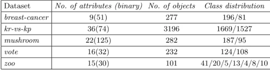
Table 1.Characteristics of datasets used in experiments

Dataset No. of attributes (binary) No. of objects Class distribution breast-cancer 9(51) 277 196/81 kr-vs-kp 36(74) 3196 1669/1527 mushroom 22(125) 282 187/95

vote 16(32) 232 124/108

zoo 15(30) 101 41/20/5/13/4/8/10

The experiments were done on selected public real-world datasets from UCI Machine Learning Repository [1]. The selected datasets are from different ar-eas (medicine, biology, zoology, politics, games). All the datasets contain only categorical attributes with one class attribute and the datasets were cleared of objects containing missing values. Basic characteristics of the datasets are de-picted in Table 1 (note that the mushroom dataset was shrunk in the number of objects due to computation time reasons). Note that “9(51)” means 9 cate-gorical and 51 binary attributes obtained by nominal scaling. The classification accuracy is evaluated using the 10-fold stratified cross-validation test [6] and the 1 _Waikato _Environment _for _Knowledge _Analysis, _available _at

(6)

following results are based on averaging 10 execution runs on each dataset with randomly ordered objects.

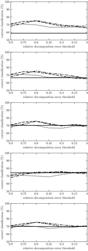
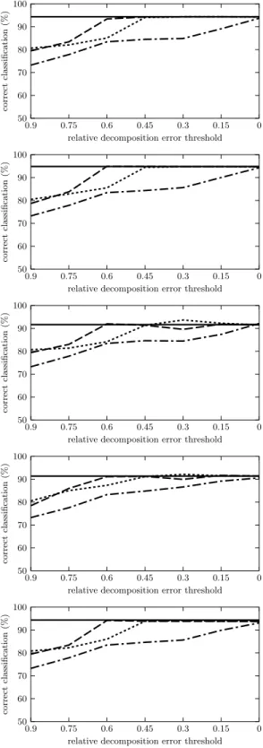
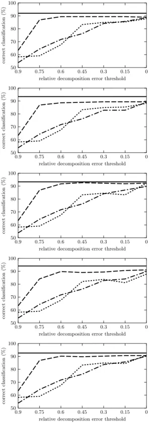
The results are depicted in Figures 1 to 5. Each figure contains five graphs for the five ML algorithms used. The graphs show the average percentage rates

of correct classifications on the preprocessed data, i.e. the data _hX, F, A, c_i

de-scribed by factors instead of_hX, Y, I, c_idescribed by the original attributes, cf.

Sections 2.2 and 2.3 for each of the three Boolean matrix factorization meth-ods. The percentage rates of GreEssQ, GreConD, and Asso are depicted by the

dashed, dot-and-dashed, and dotted lines, respectively. Thex-axis corresponds

to the factor decompositions obtained by the algorithms and, in particular, mea-sures the quantity

|hi, j_i;Iij = 1 and (A◦B)ij = 0|

|hi, ji;Iij= 1| ,

i.e. the relative error w.r.t. 1s of the input matrixI that are left uncovered in

A_◦Bfor the computed factorization given byAandB. The values on thex-axis

range from 0.9 (corresponding to a factorization with a small number of factors

that leave 90 % of the 1s inI uncovered) to 0 (corresponding to the number of

factors which decomposeIexactly, i.e.I=A_◦B). The average percentage rate

of correct classification for the original data_hX, Y, I, c_iis depicted in each graph

by a constant solid line. All the graphs are computed for the testing parts of the datasets used in the evaluation of classification only.

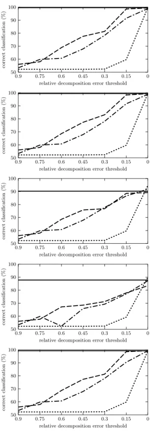
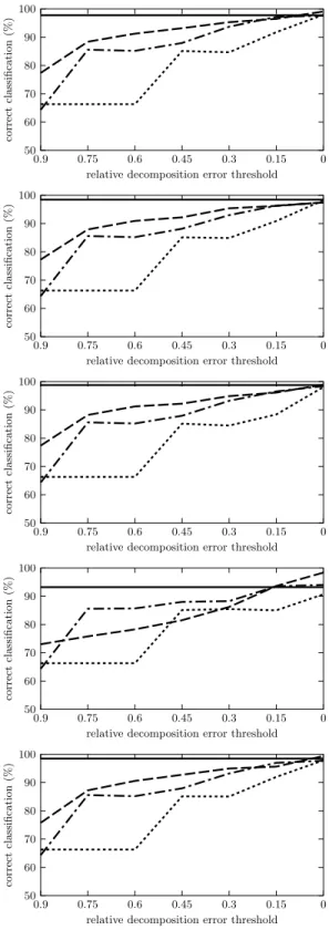
We can clearly see from the graphs for all datasets but breast-cancer that the best results (average percentage rates of correct classifications) for preprocessed data are obtained, for all ML algorithms used, by the GreEssQ algorithm, out-performing both GreConD and, quite significantly, the Asso algorithm. GreConD outperforms the Asso algorithm, again for all ML algorithms used, for datasets kr-v-kp and mushroom, but not for the vote dataset. We can also see from the graphs that sometimes the preprocessed data lead to a better classification ac-curacy than the original data even with a few factors covering less than 100 % of input data. This can be seen for instance for the kr-vs-kp dataset and Nearest Neighbor and MLP or the mushroom dataset and ID.3, Naive Bayes and MLP. See [9, 10] for indications of when, i.e. for which datasets and ML algorithms, the data with original attributes replaced by factors (computed by GreConD) covering 100 % of input data leads to a better classification accuracy compared to the original data.

Particularly interesting seem the results for the breast-cancer dataset. As we can see, the preprocessed data with factors instead of the original attributes are (much) better classified compared to the original data and that this is observable for all ML algorithms used except for Naive Bayes. Furthermore, the number of factors leading to the best average percentage rates of correct classifications is

such that the factors cover just 40 % (which corresponds to 0.6 on thex-axis) of

input data! This indicates either many superfluous attributes or large noise in the input data that is overcome by using the factors. The GreEssQ and GreConD algorithms are of comparable performance here, both outperforming the Asso algorithm.

(7)

correct

classification

(%)

relative decomposition error threshold 0.9 0.75 0.6 0.45 0.3 0.15 0 50 60 70 80 90 100 correct classification (%)

relative decomposition error threshold 0.9 0.75 0.6 0.45 0.3 0.15 0 50 60 70 80 90 100

Fig. 1.Classification accuracy for breast-cancer dataset, for (from top to bottom) ML algorithms ID.3, C4.5, NN, NB and MLP

(8)

correct

classification

(%)

Fig. 2.Classification accuracy for kr-vs-kp dataset, for (from top to bottom) ML al-gorithms ID.3, C4.5, NN, NB and MLP

(9)

correct

classification

(%)

Fig. 3. Classification accuracy for mushroom dataset, for (from top to bottom) ML algorithms ID.3, C4.5, NN, NB and MLP

(10)

correct

classification

(%)

Fig. 4.Classification accuracy for vote dataset, for (from top to bottom) ML algorithms ID.3, C4.5, NN, NB and MLP

(11)

correct

classification

(%)

Fig. 5.Classification accuracy for zoo dataset, for (from top to bottom) ML algorithms ID.3, C4.5, NN, NB and MLP

(12)

4 Conclusions

We presented an experimental study which shows that when Boolean matrix fac-torization is used as a preprocessing technique in Boolean data classification in the scenario proposed in [9, 10], the particular factorization algorithms impact in a significant way the accuracy of classification. For this purpose, we com-pared three such algorithms from the literature. In addition to demonstrating further the usefulness of Boolean factorization for classification of Boolean data, the paper emphasizes Boolean factorization as a data dimensionality reduction technique that may be utilized in a similar way as the matrix-decomposition-based methods designed for real-valued data.

An extended version of this paper will include further factorization algo-rithms in the experimental comparison (let us note in this respect that a techni-cal problem with some such algorithms is that they are poorly described in the literature). Furthermore, we intend to investigate and utilize further appropriate transformation functions between the attribute and the factor spaces, in partic-ular those suitable for approximate factorizations. A comparison with other data dimensionality techniques, see e.g. the references in [12], in the presented sce-nario is also an important topic for future research. In this respect, both the impact on the classification accuracy as well as the transparency of the resulting classification model are important aspects to be evaluated in such a comparison.

References

1. Asuncion A., Newman D. J., UCI Machine Learning Repository. University of California, Irvine, School of Information and Computer Sciences, 2007.

http://www.ics.uci.edu/~mlearn/MLRepository.html

2. Belohlavek R., Vychodil V.: Discovery of optimal factors in binary data via a novel method of matrix decomposition. J. Computer and System Sci. 76(1)(2010), 3–20. 3. Belohlavek R., Trnecka M.: From-below approximations in Boolean matrix

factor-ization: geometry, heuristics, and new BMF algorithm (submitted).

4. Ganter B., Wille R.: Formal Concept Analysis. Mathematical Foundations. Springer, Berlin, 1999.

5. Kim K. H.:Boolean Matrix Theory and Applications.M. Dekker, 1982.

6. Kohavi R.: A Study on Cross-Validation and Bootstrap for Accuracy Estimation and Model Selection. Proc. IJCAI1995, pp. 1137–1145.

7. Mitchell T. M.:Machine Learning.McGraw-Hill, 1997.

8. Miettinen P., Mielik¨ainen T., Gionis A., Das G., Mannila H., The Discrete Basis Problem. IEEE Trans. Knowledge and Data Eng. 20(10)(2008), 1348–1362 (pre-liminary version in PKDD 2006, pp. 335–346.)

9. Outrata J.: Preprocessing input data for machine learning by FCA. Proc. CLA 2010, pp. 187–198, Sevilla, Spain.

10. Outrata J.: Boolean factor analysis for data preprocessing in machine learning. Proc. ICML 2010, pp. 899-902, Washington, D.C., USA.

11. Quinlan J. R.:C4.5: Programs for Machine Learning.Morgan Kaufmann, 1993. 12. Tatti N., Mielik¨ainen T., Gionis A., Mannila H.: What is the dimension of your