Volume 4 - Article 10 | Pages 337–368

in the population sciences published by the Max Planck Institute for Demographic Research Doberaner Strasse 114 · D-18057 Rostock · GERMANY www.demographic-research.org

DEMOGRAPHIC RESEARCH

VOLUME 4, ARTICLE 10, PAGES 337-368

PUBLISHED 26 JUNE 2001

www.demographic-research.org/Volumes/Vol4/10/

DOI: 10.4054/DemRes.2001.4.10

An extension of relational methods in

mortality estimation

Harald Hannerz

1. Introduction 338

2. Proportional hazards versus proportional CDO’s: A

comparison based on mortality in a variety of subsets of the male population of Sweden in 1983

342

3. A reducible regression model: Formulation and

testing

350

3.1 The ingredients of the regression model 351

3.1.1 The standard life table 352

3.1.2 The mortality law for the female population 352

3.1.3 The relational method for the female population 353

3.1.4 The mortality law and relational method for the

male population

354

3.2 Data procedure and model selection criteria 355

3.3 Model selection for the female populations 356

3.4 Model selection for the male populations 358

4. Discussion 362

5. Acknowledgements 363

An extension of relational methods in mortality estimation

Harald Hannerz 1

Abstract

Actuaries and demographers have a long tradition of using collateral data to improve mortality estimates. Three main approaches have been used to accomplish the improvement — mortality laws, model life tables, and relational methods. The present paper introduces a regression model that incorporates all of the beneficial principles from each of these approaches. The model is demonstrated on mortality data pertaining to various groups of Swedish people holding a life insurance policy.

1 _{Department of Epidemiology and Surveillance, National Institute of Occupational Health, Lersø}

Parkallé 105, DK-2100

1. Introduction

A mortality law is a mathematical expression that describes mortality as a function of age. De Moivre made the first known contribution along this path in 1725. Many different expressions have been proposed since then (e.g. Gompertz 1825; Makeham 1867; Thiele 1872; Wittstein 1883; Pearson 1895; Perks 1932; Brillinger 1961; Heligman and Pollard 1980; Petrioli 1981; Mode and Busby 1982; Siler 1983; Anson 1988; Kostaki 1992; Hannerz 1999), and several reviews have been written on the subject (e.g. Benjamin and Haycocks 1970; Keyfitz 1982; Hartmann 1987; Kostaki 1988; Benjamin and Soliman 1993).

A model life table is simply a numerical table that gives death rates, probabilities for survival, expectations of life and other related information as a function of age. The model life tables are normally based on empirical observations in large populations believed to have reliable population and mortality data. The purpose of the model life tables is to substitute for unknown aspects of mortality in populations with limited or unreliable mortality data. The application of the models is based on the assumption that the age-pattern of mortality in the population under consideration resembles one of the life tables in the models (Adlakha 1972).

A relational method is a mathematical expression, which relates mortality in one population to that in others. In the description of relational methods as well as in the sequel of this paper, the following notations will be used: F(x) is the cumulative distribution function (cdf), which gives the probability that a person will be dead x years after birth, f(x) =DF(x) is the corresponding probability density function (pdf), and µ(x)=f(x)/(1-F(x)) is the hazard rate. The odds for death within x years after birth, F(x)/(1-F(x)), will be called the cumulative distribution odds (CDO).

The classic relation, proportional hazards, which in mathematical terms may be expressed as

)

(

1

)

(

)

(

1

)

(

x

F

x

f

x

F

x

f

j j

i i

−

=

−

α

(1)

1986). The relation was elaborated by Cox (1972) and has thereafter been known to many as ‘cox proportional hazards’. In the wake of the paper by Cox the interest for the relation among demographers was rekindled and it has subsequently been used in the study of human mortality (Vaupel, Manton and Stallard 1979; Vaupel and Yashin 1985) as well as in the construction of life tables for marriage dissolutions as a function of a variety of socio-demographic variables (Menken et al. 1981).

Equation (1) was criticised by Brass, who had observed that the ratios of the death rates in any two schedules were not constant with age but followed a more complicated course, in particular moving closer to unity for older people (Brass 1971). He also remarked that the discrepancy between (1) and reality could be quite staggering. With a set of life tables published by the United Nations (UN) (1955) he showed that the ratio of the death rate in a high mortality population to that in a low at ages 5-14 years may be twenty times as great as the corresponding value at ages 70-79 years (Brass 1969). The point of Brass’ criticism against the work of Derrick was not that the idea, that a simple relationship between different mortality patterns could be established, was wrong, but that the wrong transformation was used. Brass proposed that a more realistic relation would be obtained by

(

)

(

)

(

1

(

)

)

)

(

)

(

1

)

(

)

(

x

F

x

F

x

f

x

F

x

F

x

f

j j

j

i i

i

−

=

−

β

(2)

where i and j are defined as previously and β is a constant. Integration of (2) would then yield the equation

















−

+

=













−

1

(

)

)

(

log

)

(

1

)

(

log

x

F

x

F

x

F

x

F

j j

i

i

α

β

(3)

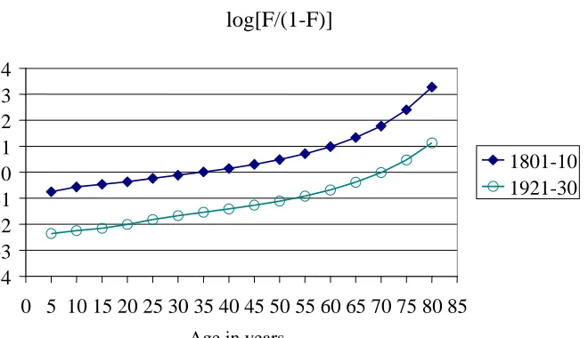
mortality changes in countries with a long series of life tables, α moved steadily with falling death rates while β fluctuated around 1 but had a strong tendency to return to this central value (Brass 1974). An illustration of this finding is given in Figure 1, where the logarithmised CDO with regard to the empiric mortality experiences of the male population of Sweden in the calendar periods 1801-10 and 1921-30 are given as a function of age. Although the median length of life had increased from 35 to 70 years between the two observation periods the curves of the logarithmised CDO of the two life tables are still approximately parallel. No smoothing has been attempted.

Figure 1: Logarithms of empirical cumulative distribution odds, with respect to the

mortality experience in the male population of Sweden in the calendar periods 1801-10 and 1921-30. Data source:(Brass, 1971).

If we fix β in (3) at its central value, one, then we obtain the simpler relation, proportional CDO’s, which mathematically may be expressed either as

log[F/(1-F)]

-4

-3

-2

-1

0

1

2

3

4

0 5 10 15 20 25 30 35 40 45 50 55 60 65 70 75 80 85

Age in years

)

(

1

)

(

)

(

1

)

(

x

F

x

F

x

F

x

F

j j

i i

−

′

=

−

α

(4)

where α’ is equal to eα in (3), or equivalently as

(

)

(

)

(

1

(

)

)

)

(

)

(

1

)

(

)

(

x

F

x

F

x

f

x

F

x

F

x

f

j j

j

i i

i

−

=

−

(5)

One can easily show that equation (4) also implies that

(

1

'

)

(

)

1

)

(

)

(

x

F

x

x

j j

i

_α

µ

α

µ

−

−

′

=

(6)

from which it is obvious that µi(x) approaches µj(x) monotonically as x approaches

infinity, a feature that, according to the writings of Brass, might be more in agreement with experience than proportional hazards. Relation (4) has been used to project future life tables from past trends (Brass 1974). It has also been used to relate mortality among survivors of myocardial infarction to that of the general population for the purpose of increased precision in life expectancy estimates (Hannerz 1996a; 1996b).

It should be mentioned that Brass did not aim at perfect goodness-of-fit, but at a simple method to obtain decent approximations. A factor analysis of the data underlying the UN-tables of 1955 had indicated that at least three factors were needed to explain about 94% of the variation between the studied mortality schedules (Lederman and Breas 1959). These factors have been interpreted as (i) a factor governing the level of mortality; (ii) a factor governing the relationship between mortality in youth and adult life; and (iii) a factor governing mortality patterns at extreme ages (especially old age, 70+). It has also been postulated that two more factors are needed to explain the rest of the observed variation; (iv) a factor governing infant mortality; and (v) a factor governing the differences between male and female mortality schedules (Pichat 1962). The work of Brass together with that of Bourgois-Pichat later inspired the enlargement of equation (3) into two different four-parameter relations (Zaba 1979; Ewbank, Gomez de Leon and Stoto 1983).

from each of the three ways previously used to improve mortality estimates — mortality laws, model life tables and relational methods.

2. Proportional hazards versus proportional CDO’s: A comparison

based on mortality in a variety of subsets of the male population of

Sweden in 1983

Sometimes statisticians are confronted with the problem of estimating mortality in small populations or in populations where mortality data do not exist for all age strata. In these situations the mortality data of the sample alone may not be enough to obtain reasonable estimates of more than one parameter, and collateral data must be used to substitute for what we do not know. As a measure of relative mortality, the odds ratios (OR) formed by dividing CDO’s in different groups will have an exact interpretation only if we regard closed populations in longitudinal studies. Most mortality studies concerns, however, only short periods, and most populations are open for non-death-related departures and/or entrance of new group members. From a mathematical viewpoint CDO’s can still be estimated from observed hazard rates and the OR’s could be used as a mortality index. The interpretation may however be questionable. As a method of graduating mortality for the purpose of life tables or estimation of life expectancies an assumption of proportionality in CDO‘s may still be useful and according to the work of Brass would often be more compatible with data than an assumption of proportional hazard rates. From this viewpoint, the present comparison could be regarded as a confirmatory analysis.

The material of the study was derived from the following three sources: a record-linkage between the Swedish national inpatient registry and the national cause of death registry 1978-83, mortality data from the Swedish Insurance Federation 1983, and mortality data from the publication “Statistical Abstracts of Sweden, 1983” (Statistics Sweden 1984). The observed outcome was deaths during the calendar year 1983.

The following subsets were regarded:

• ”Men with a history of functional psychosis”. This subset consists of men who had been psychiatric inpatients some time during the interval January 1978 - November 1982 with a diagnosis of functional psychosis (International Classification of Diseases, version eight (ICD-8)=295-299) as principal diagnosis.

1978 - November 1982 with a diagnosis related to drug abuse (ICD-8=291, 303-304) as principal diagnosis.

• ”Men with a history of acute myocardial infarction (AMI)”. This subset consists of men who had been inpatients some time during the interval January 1978 - November 1982 with a diagnosis of AMI (ICD-8=410) as principal diagnosis.

• ”Life insured men”. This data set comes from the Swedish Insurance Federation.

• ”Single men”. The data on this subset was extracted from the publication ”Statistical abstracts of Sweden 1983”.

• ”Married men”. The data on this subset was extracted from the publication ”Statistical abstracts of Sweden 1983”.

• ”Divorced men”. The data on this subset was extracted from the publication ”Statistical abstracts of Sweden 1983”.

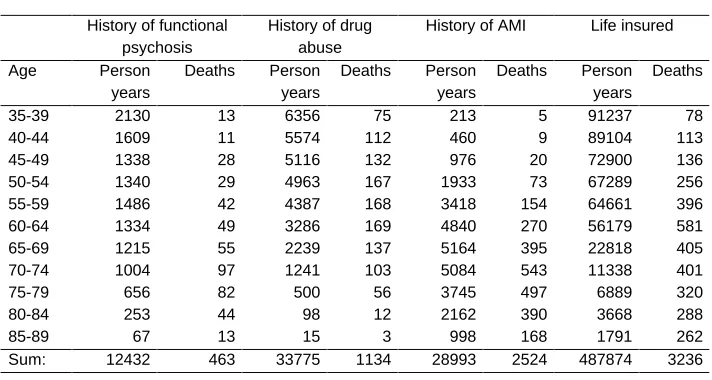
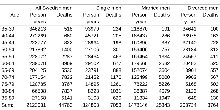
Deaths and person years at risk in the various subsets are given in Tables 1 and 2.

Table 1: Risk masses and deaths in various subsets of the male Swedish population

1983

History of functional psychosis

History of drug abuse

History of AMI Life insured

Age Person

years

Deaths Person years

Deaths Person years

Deaths Person years

Deaths

35-39 2130 13 6356 75 213 5 91237 78

40-44 1609 11 5574 112 460 9 89104 113

45-49 1338 28 5116 132 976 20 72900 136

50-54 1340 29 4963 167 1933 73 67289 256

55-59 1486 42 4387 168 3418 154 64661 396

60-64 1334 49 3286 169 4840 270 56179 581

65-69 1215 55 2239 137 5164 395 22818 405

70-74 1004 97 1241 103 5084 543 11338 401

75-79 656 82 500 56 3745 497 6889 320

80-84 253 44 98 12 2162 390 3668 288

85-89 67 13 15 3 998 168 1791 262

Table 2: Risk masses and deaths in various subsets of the male Swedish population 1983.

All Swedish men Single men Married men Divorced men

Age Person

years

Deaths Person years

Deaths Person years

Deaths Person years

Deaths

35-39 346213 518 93979 224 216870 191 34641 100

40-44 272269 660 45721 205 188437 286 36978 163

45-49 223777 822 28964 198 160896 387 32140 228

50-54 217892 1400 27106 301 159406 757 28184 313

55-59 228072 2287 28464 463 169454 1334 24567 411

60-64 239078 3969 29102 677 179568 2532 20483 525

65-69 204125 5530 23791 888 152074 3604 13901 557

70-74 177154 7832 21452 1176 125499 5000 9902 567

75-79 120785 8767 14895 1261 78222 5226 5168 502

80-84 66508 7837 8223 1031 36387 4079 2123 268

85-89 27158 5141 3108 629 11334 1947 648 130

Sum: 2123031 44763 324803 7053 1478146 25343 208734 3764

A series of graphs were made to study the appropriateness of the two relations. In creating the graphs, the hazard rate was assumed to be constant within each 5-year age category and was assessed by dividing the number of deaths by the risk mass in person years. In particular, for i,j∈{37.5, 42.5, … , 87.5}, the hazard rates were calculated by the formula µi=Di/Ni, where Di is the number of deaths occurring in the age interval (i

-2.5,i+2.5) years and Ni is the number of person years at risk in that interval. The

conditional distribution function F, for the i- and j-values in the above set, were thereafter approximated by the formula

































+

−

−

≅

>

=

∑

<j

i j

j

i i j

N

D

N

D

X

j

F

F

2

5

5

exp

1

)

35

|

(

.

Purely descriptive graphs based on the empirical hazard and distribution functions described above were created. Thereafter, the observed hazard ratios between various populations and the total population of Sweden were compared with the expected hazard ratios under the two hypotheses, proportional hazards and proportional CDO’s. The following scheme was used to calculate the expected values. Let µs,i be the hazard

rate and Fs,i be the distribution function for the age i in the standard population (all

given proportional CDO’s, µi/µs,i = β/[1-(1-β)Fs,i], where β is another constant. The

parameter γ was estimated by solving the equation

∑

=

∑

i s

i i s i

N

N

D

D

, ,

γ

,

where Di and Ni pertain to the study population while Ds,i and Ns,i pertain to the standard

population, and the parameter β was estimated by solving the equation

(

)

[

]

∑

=

∑

₋

₋

i s i

s

i i s i

F

N

N

D

D

, ,

,

1

1

β

β

.

The results of the study are given in the Figures 2 through 9.

Figure 2: Logarithms of empirical hazard rates in various subsets of the male

Swedish population 1983. If proportional hazards were true then these below would be estimates of parallel lines. If proportional CDO’s were true then these below would be estimates of lines that approach each other monotonically as age increases.

log[f/(1-F)]

-7 -6 -5 -4 -3 -2 -1

35-39 40-44 45-49 50-54 55-59 60-64 65-69 70-74 75-79 80-84 85-89

History of AMI

History of drug abuse

History of functional psychosis Divorced

Single

Married

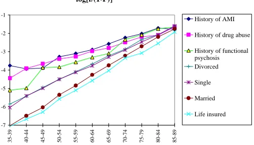
Figure 3: Logarithms of empirical CDO’s in various subsets of the male Swedish population 1983. If proportional CDO’s were true then these below would be estimates of parallel lines. If proportional hazards were true then the distances between the lines below would increase monotonically with age.

Figure 4: Hazard ratios for various subsets of the male Swedish population in

relation to the total male Swedish population 1983. If proportional hazards were true then the lines below would be estimates of parallel lines with constant values. If proportional CDO’s were true then these below would be estimates of lines that approach unity, monotonically, as age increases.

Hazard rates, f/(1-F), divided by corresponding values in the total population of Sweden

0 2 4 6 8 10 12 14 16

35-39 40-44 45-49 50-54 55-59 60-64 65-69 70-74 75-79 80-84 85-89

History of AMI

History of drug abuse

History of functional psychosis Divorced

Single

Married

Life insured

log[F/(1-F)]

-6 -4 -2 0 2 4

35-39

40-44

45-49

50-54

55-59

60-64

65-69

70-74

75-79

80-84

85-89

History of AMI

History of drug abuse

History of functional psychosis Divorced

Single

Married

Figure 5: Hazard by distribution function, f/(F(1-F)), divided by corresponding values in the total male population of Sweden 1983. If proportional CDO’s were true then f/(F(1-F)) would be independent of population, i.e. the equation for all of the lines below would be y=1.

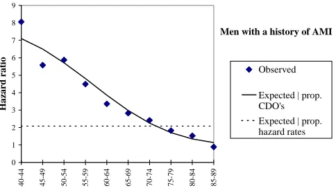
Figure 6: Observed and expected hazard ratios among men with a history of AMI

(acute myocardial infarction), in relation to the total male population of Sweden 1983.

Hazard by distribution function, f/(F(1-F)), divided by corresponding values in the total population of Sweden

0 2 4 6 8 10 12 14 16

35-39 40-44 45-49 50-54 55-59 60-64 65-69 70-74 75-79 80-84 85-89

History of AMI

History of drug abuse

History of functional psychosis Divorced

Single

Married

Life insured

Men with a history of AMI

0 1 2 3 4 5 6 7 8 9

40-44 45-49 50-54 55-59 60-64 65-69 70-74 75-79 80-84 85-89

Hazard ratio

Observed

Figure 7: Observed and expected hazard ratios among divorced men, in relation to the total male population of Sweden 1983.

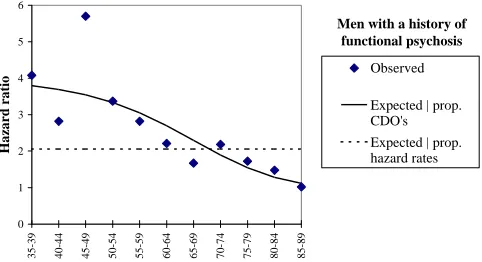
Figure 8: Observed and expected hazard ratios among men with a history of

functional psychosis, in relation to the total male population of Sweden 1983.

Divorced men

1.0 1.2 1.4 1.6 1.8 2.0

35-39 40-44 45-49 50-54 55-59 60-64 65-69 70-74 75-79 80-84 85-89

Hazard ratio

Observed

Expected | prop. CDO's Expected | prop. hazard rates

Men with a history of functional psychosis

0 1 2 3 4 5 6

35-39 40-44 45-49 50-54 55-59 60-64 65-69 70-74 75-79 80-84 85-89

Hazard ratio

Observed

Figure 9: Observed and expected hazard ratios among life insured men, in relation to the total male population of Sweden 1983.

Life insured men

0.0 0.2 0.4 0.6 0.8 1.0 1.2

25-29 30-34 35-39 40-44 45-49 50-54 55-59 60-64 65-69 70-74 75-79 80-84 85-89 90-94

Hazard ratio

Observed

3. A reducible regression model: Formulation and testing

The Swedish Insurance Federation is an institution held in common by a number of Swedish insurance companies. One of the tasks of this institution is to provide estimates for mortality risks and life expectancies of life insured clients of the concerned companies. The tables below emanating from the insurance federation give risk masses, in person years, and deaths of a population of life insured individuals in 1982, divided into three groups on the basis of how long they had been insured.

Table 3: Risk masses and deaths in cohorts of life insured Swedish males of 1982.

Insured since 11-∞ years Insured since 6-10 years Insured since 1-5 years

Age Person years Deaths Person years Deaths Person years Deaths

15-19 80.33 0 565.92 0 1373.57 1

20-24 999.84 1 2189.36 1 4433.04 1

25-29 6070.61 9 5661.81 4 11714.54 2

30-34 16738.20 10 12166.34 7 23610.69 14

35-39 34922.37 40 20666.68 29 34152.53 22

40-44 35135.33 52 18588.22 29 26018.37 17

45-49 36493.85 102 14802.46 30 16895.60 27

50-54 42250.64 144 13015.72 32 11357.22 20

55-59 48379.96 291 10627.34 63 6661.93 36

60-64 44877.44 461 7365.84 54 3946.62 25

65-69 16273.61 321 3119.58 44 2827.88 37

70-74 8053.78 290 1644.68 55 1294.20 41

75-79 5572.67 286 710.33 30 315.47 16

80-84 3272.32 301 209.00 23 74.08 7

85-89 1717.01 255 37.00 1 9.50 1

90-94 217.48 42 6.50 0 1.00 0

Table 4: Risk masses and deaths in cohorts of life insured Swedish females of 1982.

Insured since 11-∞ years Insured since 6-10 years Insured since 1-5 years

Age Person years Deaths Person years Deaths Person years Deaths

15-19 36.33 0 498.33 0 1151.66 0

20-24 868.68 0 1819.50 0 4531.08 1

25-29 4791.41 5 5370.41 2 8425.29 3

30-34 14056.37 9 9834.19 6 11336.49 1

35-39 26013.73 26 10971.96 7 13099.55 5

40-44 21636.16 19 7714.52 8 9099.53 6

45-49 18393.58 34 5760.26 4 5972.33 6

50-54 18577.74 68 5156.83 2 4159.51 5

55-59 16027.79 83 4221.09 10 2884.73 14

60-64 11716.04 64 3114.06 11 2112.13 7

65-69 4847.20 59 1524.40 13 1410.56 13

70-74 2953.41 52 954.83 14 756.17 7

75-79 1925.59 54 443.00 14 184.50 10

80-84 1152.66 94 147.58 5 72.75 6

85-89 635.99 55 39.00 4 13.50 1

90-94 71.57 13 3.00 1 1.00 0

Sum: 143704.25 635 57572.96 101 65210.78 85

In the present section, a regression model intended to incorporate the beneficial principles from each of the three ways previously used to improve mortality estimates — mortality laws, model life tables and relational methods — will be formulated, and tested on the above insurance data.

3.1 The ingredients of the regression model

3.1.1 The standard life table

It should be remembered that the incorporation of collateral data from a standard life table implies an assumption that at least some aspect of the age-pattern of mortality in the population under consideration resembles that of the standard. It is also evident that the higher the degree of similarity between the study population and the standard, the higher the advantage of its use. It has, for example, been concluded that some advantage would be gained by the use of standard life tables for each gender rather than one in common (Brass 1971), and that an African standard would be better than a European in the analysis of mortality in Africa (Zaba 1979). Another observation is that the standard itself can be improved by graduation (Hannerz 1999). In the present work, one life table for the total male population and one for the total female population of Sweden in 1982 will be used as standards for males and females respectively. The standard life tables will be graduated by the same mortality laws that will be used to graduate the mortality among the insurance policy holders.

3.1.2 The mortality law for the female population

The works of Brass, Zaba, and Ewbank et al. all imply that













−

=

)

(

1

)

(

log

)

(

x

F

x

F

x

G

(7)

is the choice transformation to work with in relational methods. The mortality law that will be used in the present work gives a five-parameter representation of the function G(x). It was empirically derived by observations on the pattern of

(

)

(

)

)

(

)

(

1

)

(

)

(

)

(

x

F

x

x

F

x

F

x

f

dx

dG

x

g

=

µ

−

=

=

(8)

in the female part of the Swedish population. The observed pattern suggested that g(x) would be (i) inversely proportional to x2 for small x (close to zero); (ii) approximately proportional to x throughout the age interval of the labour force (16-64 years) and; (iii) exponentially increasing in the very old ages (Hannerz 1999; 2001). A translation of the above scheme into the language of mathematics would produce a function consisting of three terms: a1x-2, a2x and a3ecx. In this function a1x-2 dominates in the left

out the ”straight line” and finally achieves a complete domination as x increases towards infinity. Hence,

cx

e

a

x

a

x

a

x

g

(

)

=

₁ −2

+

₂

+

₃ (9)

where a1, a3 and c are positive valued parameters and a2 is a parameter that may be

negative as long as g(x) always is greater than or equal to zero, and

cx

e

c

a

x

a

x

a

a

dx

x

g

x

G

3

2 2 1 1 0

2

)

(

)

(

=

∫

=

−

−

+

+

. (10)

By the analytical expressions given above for g(x) and G(x) we also obtain analytical expressions for the cumulative distribution function F(x)=eG(x)/[1+eG(x)], the probability density function f(x)=g(x)eG(x)/[1+eG(x)]2, the hazard function µ(x)=g(x) eG(x)/[1+eG(x)], and the survival function l(x)=1-F(x)=[1+eG(x)]-1.

Hannerz (2001) has shown that the mortality law described above nicely fits the population of Swedish females — a modern female population with low infant mortality and high life expectancy. The function has also been successfully used to graduate mortality among female survivors of acute myocardial infarction (Hannerz 1996a; 1996b), and stroke (Hannerz 1999).

3.1.3 The relational method for the female population

In harmony with Bourgois-Pichat’s interpretation of the four factors in which female mortality schedules might differ from one another, we may use (10) to obtain the four-parameter relation

c

e

x

x

x

F

x

F

x

F

x

F

cx

j j

i i

3 2

2 1 1 0

2

)

(

1

)

(

log

)

(

1

)

(

log

=

θ

+

θ

+

θ

+

θ

















−

−













−

− ₍₁₁₎

where the θi’s are parameters that denote mortality differences and c is a constant held

in common by the two mortality schedules, i and j. If the parameter θ1 in the above

expression is different from zero then the two mortality schedules would differ with regard to infant mortality; if θ2≠0 then the schedules would differ in the relationship

the mortality pattern in the old ages. The parameter θ0 would finally determine the

difference in the level of mortality. The simplest relation, proportional CDO’s would be obtained if all parameters except θ0 were zero.

If we only consider mortality among people who are older than 15 years then the parameter θ1 in (11) becomes redundant. Hence, in the present work the reducible

three-parameter relation

c

e

x

x

F

x

F

x

F

x

F

cx

j j

i i

3 2

2 0

2

)

(

1

)

(

log

)

(

1

)

(

log

=

θ

+

θ

+

θ

















−

−













−

(12)

will be used to relate mortality between female mortality schedules.

3.1.4 The mortality law and relational method for the male population

Whereas the law given by (9) would be adequate for females, Hannerz (1999) has shown that it would be inadequate for male populations. He also showed that the only reason that the law does not fit male mortality schedules is a bulge in the hazard curve, associated with the passage into manhood. Such a bulge has been observed by many researchers and is often referred to as an accident hump (e.g. Heligman and Pollard 1980; Hartmann 1987; Kostaki 1992). If we assume that there is such a thing as a manhood trial —an added hazard intentionally or unintentionally imposed on males, either by themselves or by the environment, which is associated mainly with the passage into manhood— and that some males would die as a direct consequence of such a trial. Then, mortality among males could be divided into two types: mortality from manhood trials and mortality from other causes. A function that fits a male mortality experience would thus be obtained by the following scheme: Let F1(x) be the death

distribution given that the subject will die a ”natural” death and F2(x) be the distribution

given that the death is caused by a ”manhood trial”. Let α be the probability that a death will be natural; then

F(x) =

α

F

1

(x) + (1-

α

)F

2

(x).

(

)

(

)





















+

+

−

=

+

+

−

=

+

−

+

+

=

−

+

=

c

e

a

x

a

x

a

a

x

G

c

e

a

x

a

x

a

a

x

G

e

e

e

e

x

F

x

F

x

F

cx cx x G x G x G x G 3 2 2 5 4 2 3 2 2 1 0 1 ) ( ) ( ) ( ) ( 2 1

2

)

(

2

)

(

1

1

1

)

(

1

)

(

)

(

2 2 1 1

α

α

α

α

(13)

will be used to model mortality among males. Hannerz (1999) has shown that (13) fits well when applied to the male population of Sweden. The function has also been successfully used to graduate mortality among people with mental disorders (Hannerz and Borgå 2000), and among male survivors of acute myocardial infarction (Hannerz 1996b), and stroke (Hannerz 1999).

According to Bourgois-Pichat, apart from the four factors needed to explain differences between female mortality schedules, there would be a fifth factor that governs the differences between male and female mortality. From (13) it is obvious that if we let α be equal to 1 then the expression for the male mortality law would be identical to that of the females. Hence, if we were to associate one of the parameters in (13) with that fifth factor then α seems to be the most natural choice. With respect to male mortality, Hannerz (1999) has shown that α can vary between different schedules. Because of this fifth factor, the relational method for male mortality schedules in the present work will consider potential differences, not only in the parameters a0, a2 and a3

but also in the parameter α.

3.2 Data procedure and model selection criteria

We used the likelihood ratio test to assess a smaller model against a larger one in which it is embedded. In our data, exact values did not exist for age nor for thenumber of x year old persons at risk of dying before reaching the age x+1. Therefore, all subjects in the age interval 15-19 years were considered to be exactly 17 years at the start of the observation period, the subjects in the age interval 20-24 years were considered to be 22 years etc., and "mx+Dx/2" (mx is the person years at risk and Dxis the number of deaths

3.3 Model selection for the female populations

A list of models will be given. For each model -2logL will be calculated. The first model will be the largest and all other will be submodels of the first one. The values of the parameters ai, i∈ {0,1,2,3}, and c were obtained in a mortality assessment of the

total female population of Sweden 1982 and will be regarded as deterministic. The variables y1, y2 and y3 are indicators for the three different cohorts of insurance policy

holders, i.e. yi = 1 if the person belongs to cohort i.

Model W1: Each cohort obeys its own distribution function.

(

)

c

e

y

a

2

x

y

a

x

a

y

a

y

,

y

,

y

,

x

G

cx 3 1 i i i , 3 3 2 3 1 i i i , 2 2 1 3 1 i i i , 0 0 3 2 1













₊

_θ

+













₊

_θ

+

−

θ

+

=

∑

∑

∑

= = =

Number of estimated parameters = 9

-2log L = 9345.275

Model W2: The three cohorts are related to each other by proportional CDO’s.

(

)

1 2 2 2 3 3 cx

3 1 i i i , 0 0 3 2 1

e

c

a

x

2

a

x

a

y

a

y

,

y

,

y

,

x

G













+

θ

+













+

θ

+

−

θ

+

=

∑

=

Number of estimated parameters = 5

Model W3: The distribution function is independent of cohort.

(

)

1 2 2 2 3 3 cx

0 0 3 2

1

e

c

a

x

2

a

x

a

a

y

,

y

,

y

,

x

G













+

θ

+













+

θ

+

−

θ

+

=

Number of estimated parameters = 3

-2log L = 9380.050 P-value = 4.76*10-6

Model W4: The three cohorts are related to each other and to the population of Sweden, by proportional CDO’s.

(

)

c

e

a

x

2

a

x

a

y

a

y

,

y

,

y

,

x

G

cx 3 2 2 1 3

1 i

i i , 0 0

3 2

1

=

+

∑

θ

−

+

+

=

Number of estimated parameters = 3

-2log L = 9354.994 P-value = 0.137

Model W5: The three cohorts obey the same distribution function as the population of Sweden.

(

)

c

e

a

x

2

a

x

a

a

y

,

y

,

y

,

x

G

cx 3 2 2 1 0 3 2

1

=

−

+

+

Number of estimated parameters = 0

According to the above P-values, the smallest permissible model is W4, which contains three estimated parameters. To describe the mortality of the cohorts of female insurance policy holders we thus choose a model with the following interpretation: ”The three cohorts are related to each other and to the population of Sweden, by proportional CDO’s”. Through the P-values we can also conclude that the mortality risks of the insurance policy holders differ significantly from the mean mortality risks of the Swedish population and that the mortality risks are not independent of cohort.

3.4 Model selection for the male populations

Model M1: Each cohort obeys its own distribution function.

(

)

c

e

y

a

2

x

y

a

x

a

y

a

y

,

y

,

y

,

x

G

cx 3 1 i i i , 3 3 2 3 1 i i i , 2 2 1 3 1 i i i , 0 0 3 2 1 1













₊

_θ

+













₊

_θ

+

−

θ

+

=

∑

∑

∑

= = =

(

)

c

e

y

a

2

x

y

a

x

a

a

y

,

y

,

y

,

x

G

cx 3 1 i i i , 3 3 2 3 1 i i i , 2 2 5 4 3 2 1 2













₊

_θ

+













₊

_θ

+

−

=

∑

∑

= =

(

)

( ₍ ) ₎ 2(₂₍1 ₁2₂3)₃₎ 3 2 1 1 3 2 1 1 y , y , y , x G y , y , y , x G 3 1 i i i y , y , y , x G y , y , y , x G 3 1 i i i 3 2 1

e

1

e

y

1

e

1

e

y

y

,

y

,

y

,

x

F

+













₋

_α

₋

_β

+

+













_α

₊

_β

=

∑

∑

= =

Number of estimated parameters = 12

Model M2: The three cohorts are related by parallel G1(x)’s.

(

)

1 2 2 2 3 3 cx

3 1 i i i , 0 0 3 2 1 1

e

c

a

x

2

a

x

a

y

a

y

,

y

,

y

,

x

G













+

θ

+













+

θ

+

−

θ

+

=

∑

=

(

)

5 2 2 2 3 3 cx

4 3 2 1 2

e

c

a

x

2

a

x

a

a

y

,

y

,

y

,

x

G













+

θ

+













+

θ

+

−

=

(

) (

)

( ₍ ) ₎

(

)

2(₂₍1 ₁2 ₂3)₃₎ 3 2 1 1 3 2 1 1 y , y , y , x G y , y , y , x G y , y , y , x G y , y , y , x G 3 2 1

e

1

e

1

e

1

e

y

,

y

,

y

,

x

F

+

β

−

α

−

+

+

β

+

α

=

Number of estimated parameters = 6

-2log L = 33567.311 P-value = 0.118

Model M3: The distribution function is independent of cohort.

(

)

1 2 2 2 3 3 cx

0 0 3 2 1 1

e

c

a

x

2

a

x

a

a

y

,

y

,

y

,

x

G













+

θ

+













+

θ

+

−

θ

+

=

(

)

5 2 2 2 3 3 cx

4 3 2 1 2

e

c

a

x

2

a

x

a

a

y

,

y

,

y

,

x

G













+

θ

+













+

θ

+

−

=

(

) (

)

( ₍ ) ₎

(

)

2(₂₍1 ₁2 ₂3)₃₎ 3 2 1 1 3 2 1 1 y , y , y , x G y , y , y , x G y , y , y , x G y , y , y , x G 3 2 1

e

1

e

1

e

1

e

y

,

y

,

y

,

x

F

+

β

−

α

−

+

+

β

+

α

=

Number of estimated parameters = 4

Model M4: The three cohorts are related to each other and to the population of Sweden, by parallel G1(x)’s and do not differ from the general population with regard

to the accident hump.

(

)

c

e

a

x

2

a

x

a

y

a

y

,

y

,

y

,

x

G

cx 3 2 2 1 3 1 i i i , 0 0 3 2 1

1

=

+

∑

θ

−

+

+

=

(

)

c

e

a

x

2

a

x

a

a

y

,

y

,

y

,

x

G

cx 3 2 2 5 4 3 2 1

2

=

−

+

+

(

)

( ₍ ) ₎

(

)

2(₂₍1 ₁2 ₂3)₃₎ 3 2 1 1 3 2 1 1 y , y , y , x G y , y , y , x G y , y , y , x G y , y , y , x G 3 2 1

e

1

e

1

e

1

e

y

,

y

,

y

,

x

F

+

α

−

+

+

α

=

Number of estimated parameters = 3

-2log L = 33580.906 P-value = 4.70*10-3

Model M5: Same as model M2, but with β=0.

(

)

1 2 2 2 3 3 cx

3 1 i i i , 0 0 3 2 1 1

e

c

a

x

2

a

x

a

y

a

y

,

y

,

y

,

x

G













+

θ

+













+

θ

+

−

θ

+

=

∑

=

(

)

5 2 2 2 3 3 cx

4 3 2 1 2

e

c

a

x

2

a

x

a

a

y

,

y

,

y

,

x

G













+

θ

+













+

θ

+

−

=

(

)

( ₍ ) ₎

(

)

2(₂₍1 ₁2 ₂3)₃₎ 3 2 1 1 3 2 1 1 y , y , y , x G y , y , y , x G y , y , y , x G y , y , y , x G 3 2 1

e

1

e

1

e

1

e

y

,

y

,

y

,

x

F

+

α

−

+

+

α

=

Number of estimated parameters = 5

Model M6: Same as model M2, but with β=b2=0.

(

)

(

)

c

e

a

2

x

a

x

a

y

a

y

,

y

,

y

,

x

G

cx 3 3 2 2 1 3 1 i i i , 0 0 3 2 1

1

=

+

∑

θ

−

+

+

+

θ

=

(

)

(

)

c

e

a

2

x

a

x

a

a

y

,

y

,

y

,

x

G

cx 3 3 2 2 5 4 3 2 1

2

=

−

+

+

+

θ

(

)

( ₍ ) ₎

(

)

2(₂₍1 ₁2 ₂3)₃₎ 3 2 1 1 3 2 1 1 y , y , y , x G y , y , y , x G y , y , y , x G y , y , y , x G 3 2 1

e

1

e

1

e

1

e

y

,

y

,

y

,

x

F

+

α

−

+

+

α

=

Number of estimated parameters = 4

-2log L = 33570.282 P-value = 0.107

Model M7: The three cohorts obey the same distribution function as the population of Sweden.

(

)

c

e

a

x

2

a

x

a

a

y

,

y

,

y

,

x

G

cx 3 2 2 1 0 3 2 1

1

=

−

+

+

(

)

c

e

a

x

2

a

x

a

a

y

,

y

,

y

,

x

G

cx 3 2 2 5 4 3 2 1

2

=

−

+

+

(

)

( ₍ ) ₎

(

)

2(₂₍1 ₁2 ₂3)₃₎ 3 2 1 1 3 2 1 1 y , y , y , x G y , y , y , x G y , y , y , x G y , y , y , x G 3 2 1

e

1

e

1

e

1

e

y

,

y

,

y

,

x

F

+

α

−

+

+

α

=

Number of estimated parameters = 0

According to the above P-values, the smallest permissible model is M6, which contains four estimated parameters. To describe the mortality of the cohorts of male insurance policy holders we thus choose a model with the following interpretation: “The three cohorts are related to each other by proportional CDO’s but differ from the population of Sweden with respect to the mortality pattern in the old ages”. Through the P-values we can also conclude that the mortality risks of the insurance policy holders differ significantly from the mean mortality risks of the Swedish population and that the mortality risks are not independent of cohort.

4. Discussion

Bourgois-Pichart (1962) asserted that five factors are needed to explain observed variation between mortality schedules. The present paper suggests a new relational method with one parameter to estimate for each of these factors. As part of a regression model, which also incorporates data from a standard life table, the method was demonstrated on mortality among life insured people in Sweden. The genders were treated separately and life-tables for the total Swedish male/female population were used as standards. The results confirm earlier observations that populations with considerable differences in the level of mortality can still be associated with a high degree of similarity with respect to the shape of the mortality curve. For each cohort of life insured females we needed only to estimate one parameter, and for the males four parameter estimates were enough to describe mortality in three cohorts.

The relational method that was used was intertwined with a law of mortality. Besides yielding an increased statistical precision, mortality laws often have the following advantages:

• The mortality data for each person can be treated as an individual record. Hence there is no need to aggregate the data into age groups, and individual-based ages and follow-up periods can be used in the analysis.

• A mathematical expression for the survival function is obtained with which probabilities for death can be calculated for any age and any risk period.

convenient method to transform abridged life tables into unabridged ones. Another advantage is that smoothness of the curve is obtained, which makes the table look better. This feature is especially appreciated in the insurance industry in that insurance tables seem more reasonable when the premium rises steadily rather than irregularly with age (Keyfitz 1982). ”… if the object of graduation be restricted to a practical instrument, there would be no doubt of the superiority of the curve-fitting method, yielding as it does a perfect smoothness impossible of attainment by any other method” (Perks 1932).

Mortality laws have, however, also been subject to some severe criticism: “Elaborate models requiring many constants to be determined are useless. This rules out the whole range of attempts to express mortality as a mathematical function of age from Gompertz onwards,” (Brass 1974).

It must be admitted that the laws that were used in the present work would have been useless if they had been the only ingredients of the statistical model. It would, for example, have been clearly impossible to ascertain sensible estimates for all of the eight constants involved in the law that was used for the males if those estimates had to be based on nothing but one of the direct data sets given in Table 3. If, on the other hand, we regard mortality data from large populations, like the total population of Sweden that contains more than 4 million males, then the eight parameters are not too many, especially when compared to the un-graduated national life table, which in fact involves estimation of one parameter for each of one hundred age groups.

The key point of the present paper is that it is not necessary to choose between the application of a model life table, a relational method or a mortality law. You can use them all simultaneously.

5. Acknowledgements

References

Adlakha A. (1972). “Model life tables: an empirical test of their applicability to less developed countries.” Demography, 9:589-601.

Ajne B, Ohlin J. (1990). Livförsäkringsmatematik. Stockholm: Department of Insurance Mathematics and Mathematical Statistics. Stockholm University, Sweden.

Allebeck P, Wistedt B. (1986). “Mortality in schizophrenia. A ten year follow-up based on the Stockholm county inpatient register.” Arch Gen Psych, 43:650-653.

Anson J. (1988). “The parameters of death: a consideration of the quantity of information in a life table using a polynomial representation of the survivorship curve.“ Statistics in Medicine, 7:895-912.

Babigian HM, Odoroff CL. (1969). “The mortality experience of a population with psychiatric illness.” Am J Psychiatry, 126:470-480.

Benjamin B, Haycocks HW. (1970). The analysis of mortality and other actuarial statistics. London: Cambridge University Press.

Benjamin B, Soliman AS. (1993). Mortality on the move: methods of mortality projection. Oxford: Actuarial Education Service, Napier House, England. Bourgois-Pichat J. (1962). Factor analysis of sex-age specific death rates, Population

Bulletin of the United Nations, No. 6.

Brass W. (1969). A generation method for projecting death rates. In: Bechhofer F. editor, Population growth and the brain drain. Techniques and Methods of study. Birmingham: Edinburgh University Press: 75-91.

Brass W. (1971). On the scale of mortality. In: Brass W, editor. Biological aspects of mortality. Symposia of the society for the study of human biology. Volume X. London: Taylor & Francis Ltd.: 69-110.

Brass W. (1974). “Mortality models and their uses in demography.” Transactions of the Faculty of Actuaries, 33:122-133.

Brillinger DR. (1961). “A justification of some common laws of mortality.” Trans Soc Actuaries, 13:116-119.

Derrick VPA (1927): “Observation on (1) Errors of Age in the Population Statistics of England and Wales, and (2) the changes in Mortality indicated by the national records.” Journal of the Institute of Actuaries, 58:117-146.

Ewbank DC, Gomez de Leon JC, Stoto MA. (1983). “A reducible four-parameter system of model life tables.“ Population Studies, 37:105-127.

Gompertz B. (1825). “On the nature of the function expressive of the law of human mortality.” Philosophical Transactions, 27:513-519.

Hannerz H. (1996a). Korttidsdödlighet bland hjärtinfarktpatienter vid svenska akutsjukhus 1987-91. Stockholm: Socialstyrelsen.

Hannerz H. (1996b). Korttidsdödlighet bland hjärtinfarktpatienter vid svenska akutsjukhus 1992-94. Stockholm: Socialstyrelsen.

Hannerz H. (1999). Methodology and applications of a new law of mortality. Lund: Department of Statistics. University of Lund, Sweden.

Hannerz H. (2001). “Presentation and derivation of a five-parameter survival function intended to model mortality in modern female populations.” Scandinavian Actuarial Journal, (In press)

Hannerz H, Borgå P. (2000). ”Mortality among persons with a history as psychiatric inpatients with functional psychosis.” Social Psychiatry and Psychiatric Epidemiology, 35:380-387.

Hartmann M. (1987). “Past and recent attempts to model mortality at all ages.” Journal of Official Statistics, 3:19-36.

Heligman M, Pollard JH. (1980). “The age pattern of mortality.” Journal of the Institute of Actuaries 107: 49-80.

Kermack WO, McKendrick AG, McKinlay PL. (1934). “Death rates in Great Britain.” Lancet, 1:698-703.

Keyfitz N. (1977). Applied mathematical demography. New York: John Wiley & Sons. Keyfitz N. (1982). “Choice of function for mortality analysis: Effective forecasting

depends on a minimum parameter representation.” Theoretical population Biology, 21:329-352.

Kostaki A. (1991). “The Heligman-Pollard formula as a tool for expanding an abridged life table.” Journal of Official Statistics, 7:311-323

Kostaki A. (1992). Methodology and applications of the Heligman-Pollard formula. Lund: Department of Statistics. University of Lund, Sweden.

Larsen RJ, Marx ML. (1986). An introduction to mathematical statistics and its applications. New Jersey: Prentice-Hall, Englewood Cliffs.

Ledermann S, Breas J. (1959). “Les dimensions de la mortalite.” Population, 14:637-682.

Makeham WM. (1867). “On the law of mortality.” Journal of the Institute of Actuaries, 13:335-340.

Menken J, Trussel J, Stempel D, Babakol O. (1981). ”Proportional hazards life table models: an illustrative analysis of socio-demographic influences on marriage dissolution in the united states.” Demography, 18:181-199.

Mode C, Busby R. (1982). ”An eight parameter model of human mortality— the single decrement case.” Bulletin of Mathematical Biology, 44:647-659.

Pearson, K. (1895). “Contributions to the mathematical theory of evolution. II. Skew variation in homogenous material.” Philosophical Transactions of the Royal Society of London, 186:343-414.

Perks W. (1932). “On some experiments in the graduation of mortality statistics.” Journal of the Institute of Actuaries, 63:12-57.

Petrioli L. (1981). A new set of models of mortality. Paper presented at IUSSP seminar on methodology and data collection, Dakar, Senegal, reprinted by Universita degli Studi di Siena, Italy.

Siler W. (1983). “Parameters of mortality in human populations with widely varying life spans.” Statistics in Medicine, 2:373-380.

Thiele TN. (1872). “On a mathematical formula to express the rate of mortality throughout life.” Journal of the Institute of Actuaries, 16:313-329.

United Nations. (1955). Age and sex pattern of mortality, Population Studies No. 22. New York.

Vaupel JW, Yashin AI. (1985). “Heterogeneity’s ruses: some surprising effects of selection on population dynamics.” The American Statistician, 39:176-185. Wittstein J. (1883). “The mathematical law of mortality.” Journal of the Institute of

Actuaries, 24:152-173.