in the population sciences published by the Max Planck Institute for Demographic Research Doberaner Strasse 114 · D-18057 Rostock · GERMANY www.demographic-research.org
DEMOGRAPHIC RESEARCH
VOLUME 7, ARTICLE 9, PAGES 379-390
PUBLISHED 20 AUGUST 2002
www.demographic-research.org/Volumes/Vol7/9/
DOI: 10.4054/DemRes.2002.7.9
Descriptive Findings
Twins or two single children:
the influence of the multiplicity of the first birth
on the divorce risk of Swedish women
Rainer Walke
1 Introduction 380
2 Data and methods 381
3 Impact of twins on the divorce risk 382
4 Conclusions 386
5 Acknowledgments 386
Appendix 387
Descriptive Findings
Twins or two single children: the influence of the multiplicity of the
first birth on the divorce risk of Swedish women
Rainer Walke1
Abstract
Based on Swedish register data, we compared the influence of a twin birth on the divorce risk with the influence of the sequential birth of two single children. The divorce risk for a woman with a very young child was lower than the risk for women without children or women with children older than 3.5 years. This behaviour was essentially independent of the number of children and whether or not the woman gave birth to twins. The effect of parity was much smaller than the effect of child age. The influence of twins on the divorce risk appeared to fall between that of a first and a second singleton.
1 Max Planck Instute for Demographic Research, Doberaner Str. 114, D-18057 Rostock, Germany.
1. Introduction
The main purpose of this paper is to investigate the difference between the intensity of divorce for Swedish women who gave birth to twins, and women who gave birth to two children in separate births. Often, mothers of twins are excluded from marriage disruption studies (Andersson, 1997; Andersson and Woldemicael, 2001) due to a presumption that they behave differently, and yet one does not really know where they fall within the established categories of parity in such studies.
To our knowledge, there is no study that compares the varying influence of twins and singletons on the divorce risk for mothers. Other types of studies do use twins as a natural experiment. Bronars and Grogger (1994) investigated the influence of unplanned children on the life choices of unmarried women. Using a technique derived by Rosenzweig and Wolpin (1980) they compared twin mothers with a randomly selected control sample of unmarried women with single first births. In particular, they examined the potential effect upon labour-force participation, education and the propensity for a later marriage, poverty, and welfare receipts. They considered the birth of twins to be an ‘exogenous’ fertility event. Further more, they assumed that parents distribute their attention and energy equally among their children. This method proved useful in investigating the economic impact of unplanned births. Nevertheless, their findings only apply to economic events. Though divorces are certainly influenced by economic factors, these are not the only factors.
Some events pose real emotional and economic challenges for a family. Such challenges can be a serious illness, a new job forcing relocation to another town, unfaithfulness, or loosing ones home in a fire or flood. The birth of a child is a particularly important challenge. The couple may react in different ways to such an event and their reaction may be subject to change. One such possible reaction is the increase or decrease of the propensity to divorce. Generally, we expect a reduction of the divorce risk after the birth of a child at least for some time.
Having twins could be a much more stressful event than having two singletons. The additional stress caused by having twins instead of singletons may reduce the binding effect. On the other hand, additional responsibility for two children may also serve to reduce the divorce risk.
The relationship between children and marriage stability is a reciprocal one. The birth of children has an impact on marriage stability, but the latter also influences the number of children which a couple has. Since our primary interest is in comparing singletons and twin births, the potential endogeneity of children is neglected here.
2. Data and methods
We have used a data set derived from Swedish population registers. This set covers all women born between January 1945 and December 1985 who have ever been registered as living in Sweden. For every woman we know her date of birth, her country of birth, and all of her children’s dates of birth. Additionally, we know whether and when she immigrated to Sweden or emigrated away from Sweden, her dates of marriage and divorce, and whether she herself or any current or former husband is deceased. For all these events, we know the exact year and month.
We then created a data subset containing all women with twins at first parturition and a random sample drawn from all other women. This subset contains a total of 104,970 women and it includes 14,536 mothers with twins at first birth. The size of the comparison group is six times the ‘twins-at-first-birth’ group. Therefore, it includes a sufficient number of parity 2 women with two single children. About twenty-eight percent of all women have parity 2 at the end of the study. A slight difference between the group sizes does not result in a substantial loss of analytical power (Piantadosi 1997).
For the hazard or intensity regression analysis of the risk of divorce in a woman’s first marriage, we restrict the set to those women who married at least once. The marriage spell ends either with a divorce, through the death of either spouse, with a third pregnancy, or emigration, or is censored nine months before December 1999, which is the end of the period of data collection. Within these parameters, there are 40,226 valid intervals of marriage. A total of 7,850 mothers gave birth to twins (at first birth).
For our analysis we use a proportional hazard model. In this model, the risk probability of a woman to get divorced depends on the following factors: duration of the marriage, current age, calendar year, whether she was born in Sweden, and whether or not she has had children before her first marriage. Additionally, if she has children, the divorce risk depends on the age of the first single child, the age of the second single child, and in case of twins at first birth, on their age as well. For most of these properties, we use piecewise-linear duration splines. Assuming you have enough nodes, they adjust to any pattern in the data set.
The mathematical representation of the exponential-regression formula (cf. Hoem 1987) for the divorce intensity of a woman i at exact marriage duration t (years) is:
( )
( )
( )
=
∑
= m j ji ji
t
t
x
t
1
0
exp
β
µ
We used a piecewise linear approximation
γ
(t
)
to the baseline log-intensityln
µ
0( )
t
. Each woman is characterised by seven variables. Therefore the intensity formula reads:( ) ( )
(
)
(
)
(
)
(
)
(
)
ln
1 1 3 3 4 4 5 5 6 6 7 72 i x i i i i i
i
t
=
γ
t
+
β
x
+
s
t
+
t
+
s
t
−
t
+
s
t
−
t
+
s
t
−
t
+
s
it
+
t
µ
.The time variable t counts the time since marriage. The other time variables t3i…t7i
denote a woman specific time shift. The reference category is a woman of age 30, in 1980, without premarital children and born in Sweden. The binary variable x1i is 1 if
woman i was not born in Sweden. The following spline s3 covers the dependence on the
current age of woman i. The following three splines are conditional splines. Until a certain event, they are zero. When that event occurs, they spike and continue as a piecewise linear spline. The spline s4 starts at the birth of the first singleton child if any,
and t4i is the duration of marriage of woman i at the time of birth. A negative number
denotes birth before marriage. Similarly, the spline s5 starts at any second singleton
birth. If a woman has twins in the first birth, the spline s6 starts. The last spline s7 forms
an interaction term. A binary variable x2i is 1 if woman i gave birth to a child before her
first marriage. This variable interacts with a spline that denotes the influence of the specific calendar year. Therefore we have two different splines depending on x2i, s70 in
case of a woman without a premarital birth and s71 in case of a woman with a premarital
birth. The time shift t7i denotes the duration between 1 January 1980 and marriage
formation. The splines, s3…s70,s71, shift over time by t3i…t7i depending on the history of
woman i. The nodes of all splines were pre-specified by us. We adjusted them by hand to achieve a sufficient representation of the spline shape. (A spline with n nodes needs
n+1 slope parameters; but the interaction term contains n+1 slope parameters for each
spline s70 and s71. Additionally, the splines V4, s5, s6 and s71 have an intercept
parameter.) The aML program (Lillard and Panis, 2000) varies all of these slope parameters as well as 1 to get the maximum likelihood estimates for these parameters.
3. Impact of twins on the divorce risk
We expect that the influence of having a singleton at first birth on divorce risk is similar to that of having twins. Possibly, the extra stress caused by twins increases this risk and the increasing responsibility reduces it again. Having a second singleton could have a different effect because it is not a ‘maximum challenge’ event. In order to get a clear pattern, we have to control for the following well-known influences on divorce risk as well.
Figure 1 shows the logarithmic divorce intensity dependent on marriage duration
Sweden, without children, it shows the real divorce risk per year valid for 1980. For example, in the fifth year of marriage 3.3 percent of all married such women divorce. Understandably, the divorce probability is very low immediately after marriage. It increases rapidly and reaches a maximum after about three years, after which it stays roughly constant and decreases slowly only after fifteen years of marriage. Detailed estimate values can be found in our appendix.
Figure 1: Divorce risk per year for Swedish women, by duration of first marriage.
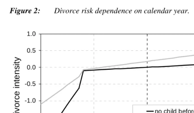
Figure 2 shows the logarithmic effect of the calendar year on the divorce intensity. It
uses a baseline year of 1980 and the baseline intensity mentioned above. In order to show that legal changes introduced in the early 1970’s have different impacts on different groups of women, we divided women into two groups: (a) with a premarital child and (b) without a premarital child. The black curve denotes women who had not given birth before marriage, while the grey curve shows the calendar effect for women who had at least one child before marriage. The divorce risk (black curve) increases rapidly between 1970 and 1973. This could be the result of a general value change regarding marriage and divorce. There is a jump upwards at the end of 1973, which may have been caused by the liberalisation of the divorce law in Sweden at that time (Sveriges Riksdag 1973). Before 1973, there were possibly an unknown number of couples waiting for better conditions to get divorced. After 1973, there is a slower increase in the risk until 1990. The grey curve does not have the same jump intensity.
-8 -7 -6 -5 -4 -3 -2
0 5 10 15 20 25 30
marriage duration in years
ln div
o
rc
e
int
e
n
s
it
y
The divorce risk gradually rises with the calendar year for women with a child before marriage. This difference between the two curves is mainly an effect of parity. Andersson (1997) showed that the strongest increase in divorce risk in 1974 was for parity 0.
Figure 2: Divorce risk dependence on calendar year.
We also include the effect of the age of a woman on the divorce risk (no figure). There is a significant additional divorce risk for younger women i.e., the risk for a twenty-year-old is approximately five times higher than that of a thirty-twenty-year-old. This risk decreases rapidly between the ages of twenty and twenty-nine. The slope then flattens, but it continues to decrease with increasing age.
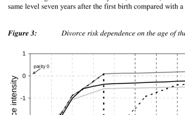
Our last figure, Figure 3, shows the effect of time since any previous birth by singleton/twin status and the order of that birth. This is the main variable of interest to us. The baseline is set at women without children. The model is extended by a summand at each birth. Technically, this is done by a duration spline starting at each birth date. This spline differs depending on which type of birth (multiple or singleton) occurs. After parturition the divorce risk is lower than for the childless baseline group. The risk then begins to increase again and plateaus after the child reaches 3.5 years. Three different curves are given in order to depict the varying effects of child age at different parities and singleton/twin status. As an example the divorce risk for a mother with two singletons 3.5 years apart is shown by a fourth, dotted curve.
-2.5 -2.0 -1.5 -1.0 -0.5 0.0 0.5 1.0
1970 1975 1980 1985 1990
calendar year
ln div
o
rc
e int
e
n
s
it
y
no child before marriage
child before marriage
All three continuous curves show a similar behaviour. Mothers with a singleton first birth have the lowest divorce risk in the months immediately following birth. The risk is higher for women who gave birth to twins. It is further higher for mothers who had a second singleton. The effect of the type of birth is reversed after 3.5 years. For mothers of only one child, it reaches a level slightly above the baseline level. In case of twins, it does not reach this baseline intensity and for the second of two singletons, it is clearly lower. The divorce risk of mothers of twins lies between that of mothers of a single child and that of mothers with a second singleton. But keep in mind that in the case of two singletons the effect of the first singleton persists after the birth of the second one. The age difference between the singletons determines the total effect. In case of an age difference of 3.5 years (dotted line) the divorce risk reaches almost the same level seven years after the first birth compared with a mother of twins.
Figure 3: Divorce risk dependence on the age of the children.
It remains for us to report the result for the binary variable that represents where the woman was born. The log-divorce-intensity of women not born in Sweden is 0.216 (standard deviation 0.037) higher than those born in Sweden. This translates into an additional risk of twenty-four percent, because exp(0.216) = 1.24.
-4 -3 -2 -1 0 1
0 1 2 3 4 5 6 7 8 9 10
time since birth in years
ln
d
iv
o
rc
e
int
e
ns
it
y
first birth, no twins second births, no twins one twin birth
two singletons 3.5 years apart
twindivR
4. Conclusions
The divorce intensity of Swedish women is strongly reduced when a child below age 3.5 years is present. Andersson (1997) showed similar results. This does not depend on whether the woman has twins or singletons. There is a smaller effect of parity. The effect of twins on the divorce risk falls somewhere between that of the first singleton and the additional effect of the second singleton.
5. Acknowledgements
I would like to thank Jan M. Hoem for his encouragement in suggesting and supporting this project. I am also grateful to Gunnar Andersson, Riccardo Borgoni, Jonathan MacGill, and Andreas Wienke for their hints and for fruitful discussions. Furthermore, I wish to thank Susann Backer and Susan Mazur for helping me edit the text of this report. I also would like to express gratefulness to two reviewers of Demographic
Research for many helpful comments and suggestions. I gratefully acknowledge the
Appendix
The following tables contain information produced by the aML program for our diagrams above. It includes the node positions, the estimates of intercepts and slope parameters, and a standard error derived by numerical computation of the Hessian matrix (Lillard and Panis 2000). Significance: ‘*’ = 10%, ‘**’ = 5%, ‘***’ = 1%.
Marriage duration (Figure 1):
log-intensity standard error
intercept -7.1395 *** 0.1799
slopes
0–1 years 2.6114 *** 0.2062
1–2 years 0.6779 *** 0.0929
2–3 years 0.4189 *** 0.0646
3–6 years 0.0062 0.0179
6–10 years -0.0340 ** 0.0141
10–15 years 0.0132 0.0132
above 15 years -0.0612 *** 0.0109
Calendar year and child before marriage (Figure 2):
child before marriage no child before marriage
log-intensity standard error log-intensity standard error
intercept 0.1759 *** 0.0465 – –
slopes
up to 1973.5 0.2315 0.1630 0.4505 *** 0.1121
1973.5–1974.0 0.5085 0.5367 1.3064 *** 0.3269
1974–1985 0.0417 *** 0.0096 0.0163 *** 0.0059
Current age (no figure):
slopes log-intensity standard error
up to 24 years -0.1947 *** 0.0212
24–29 years -0.1673 *** 0.0105
29–36 years -0.0870 *** 0.0076
36–42 years -0.0720 *** 0.0108
42–48 years -0.0624 *** 0.0171
over 48 years -0.0785 * 0.0453
Age of child (Figure 3):
first child, no twins second child, no twins twins at first birth
log-intensity standard error
log-intensity standard error
log-intensity standard error
intercept -3.8652 *** 0.4964 -2.4769 *** 0.2533 -3.0955 *** 0.6954
slopes
0–1 years 1.4508 ** 0.5720 0.3757 0.3248 0.5203 0.8719
1–2 years 1.5226 *** 0.2287 1.0359 *** 0.1943 1.5672 *** 0.4601
2–2.5 years 0.5895 ** 0.2861 0.3253 0.2839 0.8457 0.5571
2.5–3.5 years 0.6875 *** 0.0942 0.3272 *** 0.0947 0.2132 0.1676
References
Andersson, Gunnar. 1997. “The impact of children on divorce risks of Swedish women.” European Journal of Population 13: 109–145.
Andersson, Gunnar and Gebremariam Woldemicael. 2001. “Sex composition of children as a determinant of marriage disruption and marriage formation: Evidence from Swedish register data.” Journal of Population Research 18(2): 143-153.
Bronars, Stephen G. and Jeff Grogger. 1994. “The economic consequences of unwed motherhood: Using twin birth as a natural experiment.” The American Economic
Review 84(5): 1141–1156.
Hoem, Jan M. 1987. “Statistical analysis of a multiplicative model and its application to the standardization of vital rates: A review.” International Statistical Review 55: 119–152.
Lillard, Lee A. and Constantijn W.A. Panis. 2000. “aML Multilevel Multiprocess Statistical Software, Release 1.0.” EconWare, Los Angeles, California.
Piantadosi, Steven. 1997. “Sample size and power” in Clinical Trials: A Methodologic Perspective. New York, Wiley, ISBN 0-471-16393-7.
Press, William H. et al. 1992. “Least Squares as a Maximum Likelihood Estimator” in Numerical recipes in C: The art of scientific computing. 2nd ed. Cambridge University Press, 657–661, ISBN 0-521-43108-5.
Rosenzweig , Mark R. and Kenneth I. Wolpin. 1980. “Testing the quantity-quality fertility model: The use of twins as a natural Experiment.” Econometrica 48: 227–240.