Suppressing Vibration In A Plate Using Particle Swarm
Optimization
J. Javadi Moghaddam
1*and A. Bagheri
21- Phd Student Department of Mechanical Engineering, University of Guilan 2- Professor Department of Mechanical Engineering, University of Guilan
ABSTRACT
In this paper a mesh-free model of the functionally graded material (FGM) plate is presented. The
piezoelectric material as a sensor and actuator has been distributed on the top and bottom of the plate,
respectively. The formulation of the problem is based on the classical laminated plate theory (CLPT) and the
principle of virtual displacements. Moreover, the Particle Swarm optimization (PSO) algorithm is used for
the vibration control of the (FGM) plate. In this study a function of the sliding surface is considered as an
objective function and then the control effort is produced by the particle swarm method and sliding mode
control strategy. To verify the accuracy and stability of the proposed control system, a traditional sliding
mode control system is designed to suppressing the vibration of the FGM plate. Besides, a genetic algorithm
sliding mode (GASM) control system is also implemented to suppress the vibration of the FGM plate. The
performance of the proposed PSO sliding mode than the GASM and traditional sliding mode control system
are demonstrated by some simulations.
KEYWORDS
1.INTRODUCTION
The area of smart materials and structures has experienced rapid growth. Numerous researches and methods have been developed to analysis the dynamic response of the FGM and the composite plates and shells. Zhao [1] developed a free vibration analysis of metal and ceramic functionally graded plates that uses the element-free kp-Ritz method. Various numerical methods have been improved to constructing the shape function in the vibration analysis of plates and shells. The traditional numerical methods, including Ritz method, finite difference method (FDM), finite element method (FEM), etc., are applied efficiency in solving plate problems but there are still some limitations in engineering applications [2], therefore various mesh-free methods have been developed to improve the accuracy in numerical calculation of materials, including element-free Galerkin (EFG) method [3], smooth particle hydrodynamic (SPH) method [4], etc. Moreover, Liu [5] proposed the reproducing kernel particle method (RKPM), Batra et al [6] developed a modified smoothed-particle hydrodynamics (MSPH), Atluri [7] introduced meshless local Petrov-Galerkin (MLPG) method, corrective smoothed particle method (CSPM) and point interpolation methods (PIM) have been proposed by Chen [8] and Wang [9]. Bui [10] improved mesh-free methods approximation by the moving Kriging interpolation method which possesses the Kronecker’s delta property.
The EFG method is a method which uses the moving least squares (MLS) approach for field approximation. In the general least-squares problem, the output of a linear model is given by the linearly parameterized expression. Although the least-squares methods for linear approximation are the most widely used techniques for fitting a set of data, occasionally it is appropriate to assume that the data are related through a system with nonlinear parameters, Therefore quadratic polynomial basis is utilized to improve approximation and to satisfy C1 continuity [11].
In the current work, the particle swarm optimization technique is employed for the vibration control of the (FGM) plate. PSO is a population-based stochastic search algorithm. When analytical approaches either do not apply or do not guarantee a global solution for nonlinear systems, stochastic search algorithms may provide a promising alternative to these traditional approaches. PSO is a relatively new stochastic optimization technique. It was first introduced by Kennedy and Eberhart [12]. The algorithm is theoretically simple and computationally
efficient. It exhibits advantages for many complex engineering problems.
Newly, some methods based on particle swarm optimization have been introduced in the systems identification and the control problems. Jiang [13] proposed a chaos particle swarm optimization (CPSO) which involves combining the strengths of chaos optimization algorithm and PSO. Marinaki [14] developed a Particle Swarm Optimization vibration control mechanism for a beam with bonded piezoelectric sensors and actuators. Bachlaus [15] improved chaos particle swarm optimization (CPSO) using nonlinear programming to avoid trapping in local minima and T–S fuzzy modeling approaches for constrained predictive control.
2.MODEL DESCRIPTION
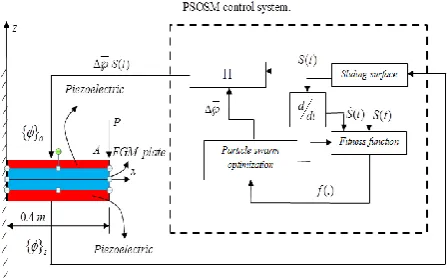
A cantilevered (CFFF) FGM plate with the integrated sensors and actuators is demonstrated in Fig.1. Top and bottom layers of the laminated plate are piezoelectric actuator layer and piezoelectric sensor layer, respectively. The region between the two surfaces is made of the combined aluminum oxide and Ti-6A1-4V materials. It is common to considering that its properties are graded through the thickness direction according to a volume fraction power law distribution. The material properties can be found in literature [16, 17, 18].
Fig. 1.The block diagram of a PSOSM control system and 2D plote of the FGM plate with distributed piezoelectric layer as an actuatore on top and a sensor on bottom.
A. Shape Functions Construction
Consider an approximation of function u(x) that is denoted by uh and expressed in discrete form as
1
( )
NP h
u
Iu
II
x
(1)
two-dimensional shape function with the kernel function is given by
( )
C
( ) (
w
)
Ix
x
x
x
I(2)
where C(x) is the correction function and is used to satisfy the reproducing condition
1
( )
for
0,1, 2.
NP
m n m n I
x y
x y
p
q
Ix
I I(3)
The correction function C(x) is described as a linear combination of the complete second-order monomial functions
( )
T(
) ( )
C
x
P
x
x
Ib
x
(4)
b(x)=[b0(x,y),b1(x,y),b2(x,y),b3(x,y),b4(x,y),b5(x,y
)]T
(5)
PT(x-xI)=[1, x-xI, y-yI, (x-xI)(y-yI), (x-xI)2, (y-yI)2]
(6)
P is a vector with a quadratic basis and is an unknown vector that to be determined. Therefore, the shape function can be obtained by the following form
( )
T( ) (
) (
w
)
Ix
b
x
P
x
x
Ix
x
I(7)
The above equation can be written as
( )
T( )
(
)
Ix
b
x
B
Ix
x
I(8)
where
(
)
(
) (
w
)
B
Ix
x
IP
x
x
Ix
x
I(9)
by substituting (8) into (3), the coefficients b(x) can be expressed by a moment matrix A and a constant vector P(0) as
1
( )
( ) (0)
b
x
A
x
P
(10)
in the above equation, A and P(0) are given by
1
( )
(
)
(
) (
)
NP Tw
A
P
IP
I II
x
x
x
x
x
x
x
(11)
(0)
1,0,0,0,0,0
TP
(12)
The tensor product weight function is expressed as
(
)
( ) ( )
w
x
x
I
w x w y
(13)
where
( )
x
x
w x
w
a
I
(14)
In this study the cubic spline function is chosen as the weight function and is given by
2 3
2 3
2 1
4 4 for 0
3 2
4 4 1
( ) 4 4 for 1
3 3 2
0 otherwise
z z z
w z z z z z
I I I
I I I I I
(15)
x
x
z
d
I I I(16)
where dI is the size of the support and can be obtained by
the following form
dI
cI(17)
where
a scaling is factor and define the basic support for node I. The shape function can therefore be written as1
( )
T(0)
( ) (
) (
w
)
P
A
P
I
x
x
x
x
Ix
x
I(18)
In this paper, the transformation method is utilized to impose the essential boundary conditions.
B. Mathematical Model Using Classical Laminated Plate Theory (Clpt)
In CLPT theory, the displacement field is presented by the following form:
0 0 1 0 2 0 3 0[
]
0
w
z
x
u
u
w
u
u
v
z
H
u
y
u
w
(19)
and
0 00
,
0,
0,
,
T
w
w
u
u v w
x
y
(20)
1
0
0
0
[
]
0
1
0
0
0
0
1
0
0
z
H
z
(21)
where
u is the midplane displacement.u v w
0,
0,
0are displacements in thex y
,
andz
directions, and w0x , 0 w y
are rotations of the
yz
andxz
planes due to bending.2 0 0 2 1 2 0 0 2 2 3 2
0 0
2
0w
u
x
x
v
w
z
y
y
u
v
w
y
x
x y
(22)
The Equations of equilibrium and electrostatics are given as follows:
,
ij j
f
biu
i
(23)
,
0
i i
D
(24)
In Quasi-static and plane stress formulations analysis, the constitutive relationship for the FGM lamina in the principal material coordinates of the lamina, is given as follows:
ij
c
ijkl kle E
ijk k
(25)
k ijk ij kl l
D
e
k E
(26)
where Ei ,i and
is the electric potential,
ij denotes stress, ij,E
i and Di are the strain, electric field and the electric displacements respectively. cijkl is the elastic coefficients, eijkand kkl are accordingly, the piezoelectric stress constants and the dielectric permittivity coefficients for a constant elastic strain. The symbol is the density of the plate which varies according to the following form,
2
( )
z
T Az
h
2
h
A
(27)
The relationship between piezoelectric stress constants and the piezoelectric strain can be obtained by the following form
31 31 11 32 12
e
d c
d c
(28)
32 31 12 32 22
e
d c
d c
(29)
In the present paper, the effective mechanical properties definitions of the plate are assumed to vary through the thickness of the uniform plate and can be written as
2
( )
2
T A A
ij ij ij ij
z
h
c z
c
c
c
h
(30)
here, simple power law distribution method is used, where
T ij c and A
ij
c are the corresponding elastic properties of the
Ti-6A1-4V and aluminum oxide, and h are the power law index and thickness of the plate, respectively.
According to the Hamilton’s principle and using above equations, the variational form of the equations of motion for the FGM plate can be written as
1 0 1 1 0 0 ti i ij ij i i t v
t t
bi i ci i
t v t
u
u
D
E
dvdt
f
u dvdt
f
u dvdt
1 00
t si it s
f
u
q
dvdt
(31)
Here q is the surface charge, t0 and t1 are arbitrary time interval, the symbol v and s represent the volume and surface of the solid respectively. fbi , fci and fsi
denote the body force, concentrated load and specified traction respectively.
C.. Discrete Governing Equation
In this section a mesh-free model of FGM plate as a plant is introduced. The displacements and electric potential at the element level can be defined in terms of nodal variables as follows
u [H N][ u]{ }ue(32)
[
N
]{ }
e(33)
where [Nu] and [N] are the shape functions, which are combined of linear interpolation functions and non-conforming Hermite cubic interpolation functions that can be found in literature [4, 6] are the EFG shape function matrices. { }e
u is the generalized nodal displacements and { }e is the nodal electric potentials.
The infinitesimal engineering strains that are associated with the displacements are given by
[Bu]{ }ue(34)
where the strain matrix [Bui][Aui]z C[ ui]and
1 2 3 4
[Bu][Bu][Bu ][Bu ][Bu ] [Au]z C[ u] for i1, 2,3 and 4. [Aui] and [Cui] are deravative matrixes of linear and non-conforming Hermite cubic interpolation functions, respectively [19].
The electric field vector
{ }
E
can be expressed in terms of nodal variables as{ }E [B ]{ }e
where [B] [N] . Substituting (25), (26), (32), (34) and (35) into (31), and assembling the element equations yields
[
M
uu]{ } [
u
K
uu]{ } [
u
K
u]{ } {
F
m}
(36)
[
K
u]{ } [
u
K
]{ } { }
F
q(37)
Substituting (37) into (36), one can obtain
1
1
[
]{ }
[
] [
][
] [
] { }
{
} [
][
] { }
uu uu u u
m u q
M
u
K
K
K
K
u
F
K
K
F
(38)
where {Fq} for the sensor and actuator layer can be
written as
{
}
[
]
0
{ }
{
}
0
[
]
{
}
{ }
[
]
0
{ }
0
[
]
{ }
q s u s s
q
u a
q a a
s s
a a
F
K
u
F
K
F
u
K
K
(39)
here, the subscript’s denotes the sensors and subscript ’a represent the actuator.
For the sensor layer, the applied charge { }Fq is zero
and the converse piezoelectric effect is assumed negligible. Using (37), the sensor output is
1
{ }
s
[
K
] [
sK
u s] { }
u
s(40)
and the sensor charge due to deformation from (37) is{
F
q}
s
[
K
u s] { }
u
s(41)
For the actuator layer, from (37), { }Fq a can be written
by the following form
{ }
F
q a
[
K
u a] { }
u
a
[
K
] { }
a
a(42)
As mentioned above and substituting (41) and (42) into (39), one can obtain
{ } [
F
q
K
u]{ } [
u
K
] { }
a
a(43)
substituting (43) into (38) and some mathematics operations one can obtain[
]{ } [
]{ } [
]{ }
{
} [
] { }
uu s uu
m u a a
M
u
C
u
K
u
F
K
(44)
where [Cs]a M[ uu]b K[ uu] is the damping matrix, a and b are Rayleigh’s coefficients.
3.CONTROL SYSTEM
A.. Sliding Mode Control System
In this section, the main problem is suppressing the vibrations and steering all states (mode shape) to equilibrium point. Therefore, a traditional sliding mode (TSM) control system is designed and fabricated to suppress the vibrations of a FGM plate. To achieve the control objective, the sliding surface can be expressed as:
2
0
( ) d t s( )
S t d
dt
(45)
where
is a positive constant. Note that, since the functionS t
0
when t0 , there is no reaching phase as in the traditional sliding-mode control [20, 21]. Differentiating S t( ) with respect to time and using (40), one can obtain:
2
( ) 2
( )
s( )
s s
S
t
t
t
(46)
1 2
2
u s
s s s
SK K u
(47)
here,
u can be expressed as:
1
) (
uu m u a a s
uu
u M F K C u
K u
(48)
substituting (47) in (46) one can obtain:
1 1 2 2 u uu s sm u a a s uu s
s
K K M
F K C
S
u K u
(49)
In this step, a control law
a
is designed so that the state to be remained on the surface S t( ) 0 for all times. Therefore, an equivalent control law
aeq
, which will determine the dynamic of the system on the sliding surface can be designed by recognizing:
|
0
a aeq
S
(50)
Substituting (50) into (49) and rearranging, the TSM control law is presented as:
1 1 1 1 1 2 ( ( ) 2 )u uu u
aeq s s a
u uu m s uu
s s
S s s
K K M K
K K M F C K u
where US sign S( ) is the robust term and is a positive constant. Thus, given S t( )0, the dynamics of the system on the sliding surface for t0 is given by:
2
( ) 2
( )
s( ) 0
s
t
st
t
(52)
The parameters of the dynamic system might be perturbed or unknown and the equivalent control law is sensitive to the unmolded dynamic and the external disturbances. Therefore, the stability of the controlled system may be destroyed.:
B. Particle Swarm Optimization Sliding Mode Control System (Psosm)
In PSO, each potential solution in an optimization problem can be visualized as a point in a D-dimensional search space and defined as a ‘‘particle’’ of the PSO. Every particle has a fitness value determined by an objective function and knows its own current best position (recorded as pbest) and current position.
In addition, every particle also knows the global best position, best, of the whole group. Every particle uses the following information to change its current location: current location, current speed, distance between the current location and its own best location and distance between the current and global best locations. The PSO search is achieved by the iteration of particle swarm, which is formed by a group of random initialized particles. The population is called the swarm and its individuals are called the particles. The swarm is defined as a set:
1 2
{ ,
,...,
N}
SW
x x
x
(53)
of N particles, defined as
1 2
(
,
,...,
) ,
T1, 2,..., .
i i i in
x
x x
x
i
N
(54)
In the proposed control system, each population is considered as a control gain. Therefore, by rewriting equations (53) and (54) one can obtain
1,
2,...,
N
SW
(55)
1,
2,...,
,
1, 2,..., .
T i i i in
i
N
(56)
The objective function, f S t
( )
, is assumed to be available for all points and is expressed as:
2 2( )
exp
(
)
f S t
S
S
(57)
here
is a small positive constant parameter ( 1) and S is the sliding surface defined in (45). The block diagram of the proposed PSOSM control system is depicted in Fig.1. This is possible by adjusting their position using a proper position shift, called velocity, and denoted as:1 2
(
,
,...,
) ,
T1, 2,..., .
i i i in
v
v v
v
i
N
(58)
Velocity is updated based on information obtained in previous steps of the algorithm. This is implemented in terms of a memory, where each particle can store the best position it has ever visited during its search. For this purpose, besides the swarm, SW, which contains the current positions of the particles, PSO maintains also a memory set:
1 2
{ ,
p p
,...,
p
N}
P
(59)
which contains the best positions?
1 2
(
,
,...,
) ,
T1, 2,..., .
i i i in
p
p
p
p
i
N
(60)
( )
arg min
(.)
i i
t
p t
f
(61)
where t stands for the iteration counter and f(.) is the objective function. The algorithm approximates the global minimizer with the best position ever visited by all particles. Therefore, it is a reasonable choice to share this crucial information. Let g be the index of the best position with the lowest function value in P at a given iteration t, the speed and position of the particle are updated based on the following formulations:
1 1 1 2 2
(
(
)
(
))
tt t t
ij
ij ij ij
t t
ij gj
v
v
k R p
k R p
(62)
1 1
t t t
ij ij
v
ij
(63)
where 2 1 2
2
,
2
4
,
4.
(64)
1k and k2 are learning factors and are all positive constant numbers and the values of R1 and R2 are randomly distributed in [0, 1]. Now, the proposed control law is presented by the following form:
where fSL( )S is a soft limit function to find the smooth control action and reduce chattering phenomena. fSL( )S can be obtained as
2
2
( )
( )
tanh
( )
1
( )
SL
S t
f
S
S t
S t
(66)
The chattering phenomenon is a particular problem in the control algorithms. The chattering problem can result in degenerate control accuracy and destroy the stability of system.
4.SIMULATION RESULTS
The present work is tried to show the performance of the proposed control system which is designed and fabricated to FGM plate to suppuration vibrations and reduction external disturbances.
G-1195N piezoelectric films bond both the top and bottom surfaces of the FGM plate as shown in Fig.1. The plate is square with both length and width set at 0.4 m. It is of thickness 5 mm, and each G-1195N piezoelectric layer is of thickness 0.1 mm. The material properties of piezoelectric and FGM materials are listed in table (1). The cantilevered (CFFF) plate is considered as the boundary condition. In this paper, a regular nodal distribution is chosen for the convergence studies. To simplify the vibration analysis, modal superposition algorithm is used, considering the first six modes in modal space. An initial modal damping for each of the modes is assumed to be 0.8%.
A unit of force P is imposed at point A of the FGM plate (Fig.1) in the vertical direction and is subsequently removed to generate motion from the initial displacement. The power law exponent for FGM plate is selected as .
In the design of proposed control systems, the effect of external disturbance are modeled as
[ ]
sin ( ) cos ( ) sin ( ) cos ( ) sin ( ) cos ( )
uu
T
d d d d d d
Dis Am K
(67)
where Am105
is the amplitude of disturbance, [Kuu] is the normalized matrix of [Kuu] , and d 200 is the
frequency of disturbance, Therefore (44) in the disturbance condition can be rewritten as
[
]{ } [
]{ } [
]{ }
{
} [
] { }
uu s uu
m u a a
M
u
C
u
K
u
F
K
Dis
(68)
here [Muu], [Cs] and [Ku]a are the normalized matrices
of [Muu], [Cs] and
[Ku]a .
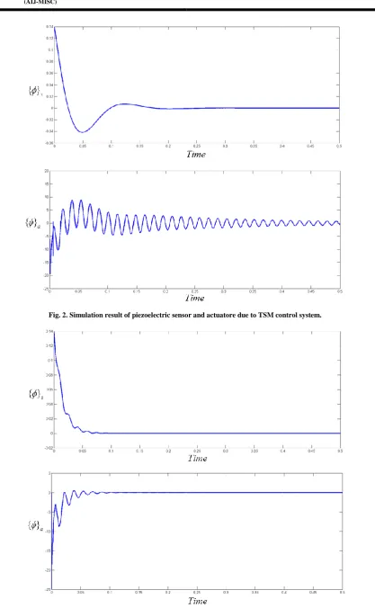
The simulation results are demonstrated in Figs. 2- 7. The effectiveness of the TSM and the PSOSM control system are depicted in Fig.2-3. The control parameter
is selected 53 and 2 for the process control with TSM and PSOSM control system, respectively. Figs.2-3 demonstrate that the settling times for the sensor output { } s are nearly 0.18 and 0.10 second due to the TSM andthe PSOSM control system, respectively. Also, in the control process, the actuator input { } a which is produced
by the PSOSM control system is less than the TSM control law.
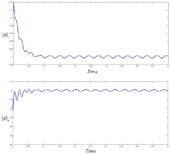
The simulation results in disturbance conditions are depicted in Fig.4-5. The harmonic response of the sensor output { } s due to the TSM control system is bounded as
[ 0.02, 0.02] . Fig.5 shows that, the variety of the sensor output { } s, due to the PSOSM control system is in
interval [ 0.005, 0.005] . Also, due to the proposed control law, a smooth control effort is produced to reduce the effect of disturbance conditions in the plant.
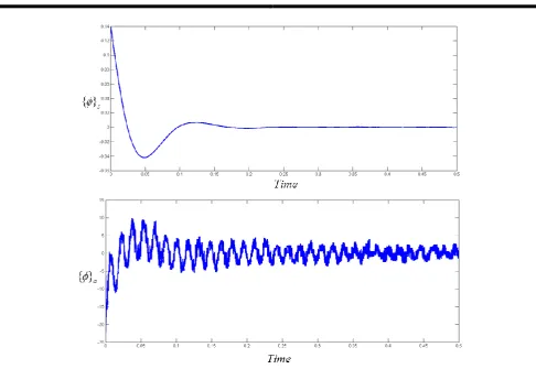
The ability of suppressing vibration in the FGM plate due to the TSM and the PSOSM control system under the random noise are depicted in Figs.6-7.
Fig. 2.Simulation result of piezoelectric sensor and actuatore due to TSM control system.
Fig. 4.Simulation result of piezoelectric sensor and actuatore due to TSM control system in disturbance conditions.
Fig. 6. Simulation result of piezoelectric sensor and actuatore due to TSM control system under the random noise
Fig. 8. Simulation result of piezoelectric sensor and actuatore due to GASM control system. TABLE 1.PROPERTIES OF THE FGM COMPONENTS
Material Properties Aluminum oxide Ti-6Al-4V G-1195N
Elastic modulus E (Pa) 11
3.2024 10 11
1.0570 10 9 63 10
Poisson’s ratio
0.2600 0.2981 0.3Density
3kg m
3750 4429 7600
31 m
d V
12254 10
32 m
d V
254 10 12
33 F
k m
915 10
and is preferred over GA when time is a limiting factor. Moreover, the fast converging and the smooth control action show that the PSOSM control system is much superior in the suppressing vibration of the FGM plate. 5. CONCLUSIONS
A general controllable mesh-free model of the FGM plate has been introduced in this paper.
A traditional sliding mode control system has been designed and fabricated to suppress the vibrations for a FGM plate in the normal, disturbed and noisy conditions. The PSOSM control system as the intelligent control approached has been successfully designed and effectively used to reject the random noise, reduce the disturbance
and finally, eliminate vibrations of the FGM plate. No constrained condition of the controlled plant is used in the design process for the proposed controller. The proposed controller can be applied in another engineering applications.
REFERENCES
[1] Zhao X., Lee Y. Y. and Liew K. M., ‘‘Free vibrationan alysis of functionally graded plates using the element-free kp-Ritz method,’’ Journal of Sound and Vibration, vol. 319, pp. 918– 939, 2009.
conforming radial point interpolation method,’’ Composites Science and Technology , vol. 68, pp. 354– 366, 2008.
[3] Belytschko T, Lu Y and Gu L. ‘‘Element-free Galerkin methods,’’ Int J Numer Methods Eng, vol. 37, pp. 229– 56, 1994.
[4] Liu G.R, Liu M.B. ‘‘Smoothed particle hydrodynamics: a meshfree particle method,’’ New Jersey: World Scientific, 2003.
[5] Liu W.K, Jun S and Zhang Y.F. ‘‘Reproducing kernel particle methods,’’ Int J Numer Methods Fluid , vol. 20, pp. 1081– 106, 1995.
[6] Batra R.C, Zhang G.M. ‘‘Analysis of adiabatic shear bands in elastothermo-viscoplastic materials by modified smoothed-particle hydrodynamics (MSPH) method,’’ J Comput Phys , vol. 201, pp. 172– 90, 2004.
[7] Atluri S. N, Zhu T. ‘‘A new meshless local Petrov-Galerkin (MLPG) approach in computational mechanics,’’ Comput Mech , vol. 22, pp. 117–27, 1998.
[8] Chen J. K, Beraun J. E and Jih C. J. ‘‘Completeness of corrective smoothed particle method for linear elastodynamics,’’ Comput Mech, vol. 24, pp. 273– 85, 1999.
[9] Wang J. G, Liu G. R. ‘‘A point interpolation meshless method based on radial basis functions,’’ Int J Numer Method Eng , vol. 54, pp. 1623– 48, 2002.
[10] Bui T. Q., Nguyen M. N., ‘‘A moving Kriging interpolation-based meshfree method for free vibration analysis of Kirchhoff plates,’’ Computers and Structures , vol. 89, pp. 380– 394, 2011. [11] K.Y. Dai, G.R. Liu, X. Han and K.M. Lim.
‘‘Thermo mechanical analysis of functionally graded material (FGM) plates using element-free Galerkin method,” Computers and Structures , vol. 83, pp. 1487– 1502, 2005.
[12] Kennedy J., Eberhart R. ‘‘Particle swarm optimization,’’ In: Proceedings of the IEEE International Conference on Neural Networks, vol. 4. Perth, Australia, pp. 1942– 1948, 1995.
[13] Jiang J., Kwong C. K., Chen Z. and Ysim Y. C. ‘‘Chaos particle swarm optimization and T–S fuzzy modeling approaches to constrained predictive control,” Expert Systems with Applications, 2011.
[14] Marinaki M., Marinakis Y and Stavroulakis G. E., ‘‘Vibration control of beams with piezoelectric sensors and actuators using particle swarm optimization,” Expert Systems with Applications, vol. 38, pp. 6872–6883, 2011.
[15] Bachlaus M., Shukla N., Tiwari M. K. and Shankar R. ‘‘Optimization of system reliability using chaos-embedded self-organizing hierarchical particle swarm optimization,” Proceedings of the institution of mechanical engineers , vol. 220, pp. 77– 91, 2006.
[16] Chen J. S., Pan C., Wu C. T. and Liu W. K. ‘‘Reproducing kernel particle methods for large deformation analysis of nonlinear structures,’’ Computer Methods in Applied Mechanics and Engineering, vol. 139, pp. 195– 227, 1996.
[17] Liew K. M., He X. Q. and Kitipornchai S., ‘‘Finite element method for the feedback control of FGM shells in the frequency domain via piezoelectric sensors and actuators,’’ Comput. Methods Appl. Mech. Energy., vol. 193, pp. 257–273, 2004. [18] Touloukian, Y. S. Thermophysical Properties of
High Temperature Solid Materials, Macmillian, New York, 1967.
[19] Reddy, J. N., Mechanics of Laminated composite plates and shells: Theory and Analysis, 2NdEd CRC Press, Boca Raton, London New York Washington, D.C 2004.
[20] Slotine J. J. E., Li, W., Applied Nonlinear Control, Prentice-Hall, Englewood Clifs, NJ, 1991.