٭Corresponding Author, Email: [email protected]
A Robust Adaptive Observer-Based Time Varying Fault
Estimation
Dr. Montadher Sami Shaker
1*1- Dept. of Electrical Engineering, University of Technology, Baghdad, Iraq
ABSTRACT
This paper presents a new observer design methodology for a time varying actuator fault estimation. A
new linear matrix inequality (LMI) design algorithm is developed to tackle the limitations (e.g. equality
constraint and robustness problems) of the well known so called fast adaptive fault estimation observer
(FAFE). The FAFE is capable of estimating a wide range of time-varying actuator fault signals via
augmenting the Luenberger-observer by a proportional integral fault estimator feedback. Within this
framework, the main contribution of this paper is the proposal of new LMI formulation that incorporates the
use of
L2norm minimization: (a) to obviate the FAFE equality constraint in order to relax the design
algorithm, (b) to ensure robustness against external disturbances, (c) to provide additional degrees of
freedom to solve the infeasible optimization problem via assigning different proportional and integral fault
estimator gains. Finally, a VTOL aircraft simulation example is used to illustrate the effectiveness of the
proposed FAFE.
KEYWORDS
1. INTRODUCTION
Owing to the increasing demand for maintaining reliable controlled system performances under different operating conditions, the last two decades have witnessed an increasing in interest in fault tolerant control (FTC) and, its complementary part, fault detection and diagnosis (FDD) [1-5].
In the literature, many approaches have been proposed for FDD purposes. Recently, the observer-based FDD approach has gains a lot of research attention [6-10]. From fault estimation standing point, there are two observer-based fault estimation approaches. One of the approaches feeds the residual signal, generated by fault detection observer, either to a static gain or to a dynamic filter to produce fault estimate. The second approach is based on the use of adaptive observer in which the estimation of the fault added to the internal observer dynamics [4-5,11-12]. In the two approaches, dealing with time varying fault signal is of paramount importance since the fault estimation accuracy highly affected by the time behaviour of fault signals. Within this framework, some FDD methods have been proposed under the common assumption of constant or slowly varying fault behaviour. In fact, such FDD methods have limited applicability, especially if the estimated fault has utilized in a fault compensation loop. The design of FAFE using LMI formulation that takes into account the effect of the fast time varying fault has been considered in [12]. However, the need for a matrix equality constraint to derive the LMI has lead to increase the design conservatism. Additionally, the effects of external disturbances on fault estimation accuracy has not been taken into account in [12].
In fact, an FDD system’s robustness against exogenous input is one of the most important diagnostic issues, especially when the diagnosis becomes a part of an FTC loop; see for example [4-5,13-14]. Moreover, in order to ensure feasible LMI solution, minimizing LMI constraints and relaxing the design conservatism has gained increased researcher’s interest [15-17].
Within this framework, in comparison with the work presented in [12], the contribution of this paper is the proposal of new LMI formulation for the FAFE observer to achieve: (1) robustness against external disturbances via
2
L norm minimization; (2) LMI conservatism relaxation
through obviating the matrix equality constraint; (3) Increase the design freedom.
The paper is presented as follow, Section 2 gives an illustration to the motivation for this work. Section 3, a
simulation results are given to show the effectiveness of the proposed algorithm.
2. PROBLEM STATEMENT AND MOTIVATIONS
This section describes the conventional FAFE developed in [1] for a linear time invariant system LTI. Let the LTI system affected by the actuator fault described as:
f a
x Ax Bu E f y Cx
(1)
where, n* n n* m n* mf p* n
f
A , B ,E ,C
are known system matrices, x (t) n,u (t) m,
p
y (t) and
mfa
f t are the state vector, input vector, output vector, and the actuator fault signal. The conventional adaptive fault diagnosis observer has the following structure:
ˆ
ˆ ˆ ˆ
ˆ ˆ
f a
x Ax Bu E f L y y
y C x (2)
where ˆx (t) n, y (t)ˆ p, and
mfa
ˆf t are the
state estimation vector, the observer output vector, and the estimated actuator fault signal. Subtracting (2) from (1), the estimation error dynamics can be given as:
x x f f
y x
e A LC e E e
e C
e (3)
where e x,e ,ey f , are the state estimation error, output estimation error, and the fault estimation error, defined as:
x
y
f a a
ˆ
e x x
ˆ
e y y
ˆ
e f f
(4)
For time varying fault scenario, the first time derivative of
f
e become:
ˆ
f a a
e f f (5)
Assumption 1 [1]: if the following assumptions satisfied
rank CE
f
mfThe pair (A, C) is observable.
The derivative of the fault with respect to time is
bounded (faf whereb 0 fb ).
then the following theorem can used to design FAFE:
Theorem 1 [1]: under the assumption given above, and scalar , 0 ,if there exist symmetric positive definite matrices P n* n,G m * mf f , and matrices
f
m * p n* p
Y , F such that the following constraints hold:
11 12
21 22
A A
A A (6)
T f
E P FC (7)
where
Y PL ,
T T
11
A PA(PA) Y C(Y C) ,
T T T
12 f f
1
A (A PE C Y E ),
21 12
T
A
A
,T
12 f f
2 1
A (E PE G),
then the FAFE algorithm
ˆ
x x
f t FC e e (8)
can make e and x ef uniformly ultimately bounded. The proof can be found in [1] and it is omitted here. However, the following lemma is required:
Lemma1: Given a scalar 0 and symmetric positive definite matrix G, the following inequality holds:
1
1
T T T T
X R R X X GX R G R (9)
where R & X are two matrices.
Remark1: (Robustness problem): The effect of the external disturbances has not been considered in the proposed observer (i.e. Eqs. 2&8) and hence it is not robust in the sense that the existence of disturbances directly affects the estimator dynamics. This would decrease the reliability of the proposed FAFE for FDD and FTC applications.
Remark2: (Solving difficulty): the equality constraint in (7), should be solved with (6) simultaneously, leading to the solving difficulty problem. In [2] a transformation
of (7) into the following LMI constraint for minimum of
0
was given:0 *
T f
I E P FC
I (10)
in fact, it is very difficult to find a feasible solution for inequalities (6) and (10) simultaneously for a minimum of
0
.Remark3: (Design freedom): since the integral and the proportional terms are governed by the same design matrices (
FC), the proposed fast fault estimation in Eq. (8) does not exploit the available design freedom.The aforementioned remarks (1, 2, and 3) have motivated us to reformulate the design such that the observer achieves the robustness requirements, relaxes the LMI design constraints, and enhances the degree of freedom so that the design problem can be solved for a wide range of tuning parameters.
3. ROBUST OBSERVER BASED FAST ACTUATOR FAULT
ESTIMATION
presents the LMI formulation for robust observer based time varying fault estimation for LTI system with bounded external disturbance. The LTI system considered here has the following form:
f a d
x Ax Bu E f E d
y C x (11)
where n* md
d
E is a known matrix and d (t) md
is the bounded disturbance input. The adaptive observer used here is given as:
1 2
ˆ
ˆ ˆ ˆ
ˆ ˆ
ˆ
f a
a x x
x Ax Bu E f L y y
y C x
f t K Ce K Ce
(12)
where f f
1 2
m * p m * p
,
K K are the proportional
and integral gains, respectively, and m * mf f is a
symmetric positive definite matrix. After subtracting the observer in (12) from the system (11) the state estimation error will be defined as:
x x f f d
y x
e A LC e E e E d
e C e (13)
1 1
2 1 1
ˆ
. ..
f a a a x x
x f f d
e f f f K CAe K CLCe K Ce K CE e K CE d
(14)
By combining Eqs. (13) & (14), the augmented estimation error dynamics can be constructed as defined in Eq.(15):
a a
e t Ae Nz (15)
where
1 1 2 1
f f
A LC E
A
K CA K CLC K C K CE
1 0 , , d x a d f a d E e K CE z I e e f N
Now the objective is to compute the gains
𝐿, 𝐾1, 𝑎𝑛𝑑 𝐾2that attenuate the effects of the input 𝑧̃, in
Eq. (15), on the estimation error via minimizing the
2norm z 2 , which should stay below a desired level
.Remark4: decoupling of disturbance effects is beyond the scope of this paper; however, based on the available information of Ef and Ed , the following theorem
ensures attenuation of disturbance effects on fault estimation signal via L2 norm minimization.
Theorem2: The augmented estimation error in (15) is stable and the L2 performance is guaranteed with an
attenuation level
, Provided that the signals
f , da
are bounded, rank CE
f
mf , and the pair (A,C) is observable, if there exists a symmetric positive definitematrices P , 1 1 and G , matrices H , K , K1 2, and a scalar
satisfying the following LMI constraint:Minimize such that
11 12 13 16
22 23 24 25
1
1
Ψ Ψ Ψ 0 0 Ψ 0
* Ψ Ψ Ψ Ψ 0 0
* * 0 0 0 0
* * * 0 0 0 0
* * * * 0 0
* * * * * 2
* * * * * * I I G P I G (16) where 1 1
LP H ,
Ψ T T
11 P A1 P A1 HC HC w1
Ψ T T T T T
12 P E1 f A C K1 C K2
Ψ Ψ T
13 P E1 d, 16 HC
Ψ T
22 K CE1 f K CE1 f w2
Ψ Ψ 1 Ψ
23 K CE1 d, 24 , 25 K C1
Proof: to achieve the required robustness against exogenous input, the objective of the estimation performance can be represented mathematically as [3]:
a 2 T 2 T
a a
0 0
2
e
e e dt z z 0
z
(17)To tune optimization of the L2 performance against
the exogenous input z , the following weighting matrix
W has been nominated. This turns Eq.17 into the following form:
1
T 2 T
a a
2
0 0
w 0 e We dt z z 0 ; W
0 w
Let
ea be the candidate Lyapunov function for the augmented system (15)
Ta a a
e e Pe ,
with P0 ,
to achieve the required performance (17) and stability of augmented system (15) the following inequality must hold [3]:
T 2 Ta a a
e e We z z 0
(18)where 𝜐̇(𝑒̃𝑎) is the derivative of the candidate Lyapunov function which can obtained easily using Eq.15
and
ea as:
T
T
T T Ta a a a a
e e A P PA e e PNz z N Pe
(19)
Substituting Eq. (19) into inequality (18) and rearrange the result into matrix form yields:
T T
a a
T 2
A A N
z N z
e P P W P e 0
P I
(20)
inequality (20) implies the following inequality.
T
T 2
P P W P
0
P I
A A N
N
1 1 P 0 P 0 0
(22)
Substitute the corresponding values of P , A , and N
and use the following variable changes H P L , 1
in to the inequality (21) to obtain:
ij
Π
11 12 13
22 23 24
0
*
0
* * I 0
* * * I
(23) where,
T
T11 P A1 P A1 HC HC w1
T T T T T T T T T
12 P E1 f A C K1 C L C K1 C K2
T13 P E1 d, 22 K1CEf K CE1 f
1 23 K CE , 1 d 24
It is clear that (23) is not linear due to the term
T T T T
1
C L C K and its transpose. Inequality (23) can be rearranged to have the form given in inequality (24) given below:
ij
11 12 13
1
22 23 24
T T T T 1 0 0 K C *
LC 0 0 0 0
* * I 0
0
* * * I
C L
0
0 C K 0 0 0 0 0 (24) where
T T T T T
12 P E1 f A C K1 C K2
use Lemma 1 and Schur theorem to obtain (25) from (24):
ij0 (25)
where,
ij
T T
11 12 13
22 23 24 1
1
0
* 0
* * 0 0 0
* * * 0 0
* * * * G 0 * * * *
0 C L
K C I * G I
where 𝐺 is as defined in Lemma1. Now (25) is linear, but there still a need to represent the estimator gain 𝐿 in (25) in term of the variableH P L 1 . Hence, (25) is divided as
shown above, and rewritten as:
11 12 ij 22 0 *
(26)
Lemma 2. (Congruence) Consider two matrices M and
Q , if M is positive definite and if Q is a full column rank matrix, then the matrix Q * M * QT is positive definite. Furthermore, letting
1 I 0 Q 0 P
the following inequalities are held.
T ij
11 12 1
1 12 1 22 1
Q * * Q 0 P
0 P P P
(27)
Inequality (27) implies 22 0then the following
inequality holds [4-5]:
1
T
1
1 22 22 1 22
2 1
1 22 1 1 22
...
P P 0
P P 2 P
where
is a scalar(28)
Substitute (28) into (27) and use the Schur complement, then (27) holds if the following inequality holds:
11 12 1
21 1 1
22
P 0
P 2 P I 0
0 I (29)
After substitution 11, 12, 21, 22 and simple
Remark5: Compared with the work presented in [1-3], the main contributions offered by the LMI design constraint (inequality (16)) developed in this paper are:
1) A great design simplification has achieved via obviating the equality constraint from the design algorithm (see Eq. (7)). Whereas, in [1-2] it is necessary to solve inequality (10) for a minimum of
0 which is often infeasible.2) The LTI system considered in this paper is affected by both actuator fault and disturbance simultaneously. Moreover, the developed design
algorithm guarantees robustness against
exogenous inputs via the L2norm minimization
with an attenuation level (
). On the other hand, only fault estimation has been studied in [1] without considering any external disturbances effect.3) The proposed method considers different gains for the proportional and integral terms of the fault estimator (see Eq. (12)). This allows more freedom for the selection of the tuning parameters in (16).
The proposed observer in (12) guarantees accurate fault estimation of time varying signals in the presence of external disturbances. On the other hand, the work in [3] focuses only on residual signal generation without any care for fault estimation and its time varying behavior.
4. SIMULATION EXAMPLE
This section presents simulation results that illustrate the theory introduced in the previous sections using the linearized dynamic model of a VTOL aircraft in the vertical plane [1]. The state space model of the VTOL given below:
f a d
x Ax Bu E f E d y C x
(30)
where 𝑥(𝑡) = [𝑉ℎ , 𝑉𝑣, 𝑞, θ] and 𝑢(𝑡) = [δ𝑐, δ𝑙 ] are
respectively the state and the input vector, 𝑉ℎ is the
horizontal velocity, 𝑉𝑣 is the vertical velocity, q is the pitch rate, and θ is the pitch angle; collective pitch control
c
and longitudinal cyclic pitch control l. The model parameters are given as:
9.9477 0.7476 0.2632 5.0337 52.1659 2.7452 5.5532 24.4221 A
26.0922 2.6361 4.1975 19.2774
0 0 1 0
0.4422 0.1761
1 0 0 0 3.5446 7.5922
B ,C 0 1 0 0 5.5200 4.4900
0 0 0 1
0 0
f f d
0.442 0.176 0.15
1 0
3.545 7.592 0.30
E , D 0 1 , E
5.520 4.490 0.20
0 0
0 0 0
Figures given below present the results of using the proposed robust estimator for different actuator fault
scenarios f1
t ,f2
t (i.e. fa f1
t f2
t T ) given in Eqs. (31) & (32) and the external disturbance
d t shown in Figure 1. The faulty signals are nominated so that fa covers a wide range of time varying fault
scenarios such as abrupt changes, constant scale, time varying faults.
1
0 0 t 2 f t
0.3 2 t
(31)
2
0 0 t 2 f t
0.3 sint 2 t
(32)
Remark 6: the proposed observer design algorithm has been tested for the following scenarios:
Scenario 1: the LMI (16) is solved for different actuator fault estimation gains (i.e. K1 K2 in Eq.12). for this scenario the following results are obtained.
For μ0.01 and G200*diag
4 ,4
0.0086
K1 0.0028 0.0031 0.0058
0.0040 0.0047 0.0133
K2 0.1956 0.0173 0.1062
0.2528 0.0134 0.1084
L
0.1792 0.0013 0.0082
0.1819 0.0212 0.1214
1.7387 0.1671 0.9079
0.0089 0.0257 0.1863
Scenario 2: the LMI (16) is solved for similar actuator fault estimation gains (i.e. K1 K2 in
For μ0.01 and G200*diag
4 ,4
The LMI constraints were found infeasible.
Fig. 1.The disturbance signal (𝒅(𝒕) )
Firstly, the simulation considers the effect of the two
fault signals separately without considering the d t
effect. Fig. 2 shows the capability of the proposed observer to track abrupt change fault (at time = 2sec.) and constant fault signal (time > 2sec). Clearly, owing to the
time varying behaviour of fa, fa 0at time = 2sec, whereas, fa 0for time > 2sec. This in turn affects the fault estimation accuracy as stated in Eq. 15.
Fig. 3 shows the fault signals 𝑓2(𝑡) and its estimation.
In this case, fa 0 for time > 2sec and hence the estimation error always slightly deviates from zero due to
a
f 0.
Fig. 2.The 𝐟𝟏(𝐭) and its estimation
Fig. 3.The 𝐟𝟐(𝐭) and its estimation
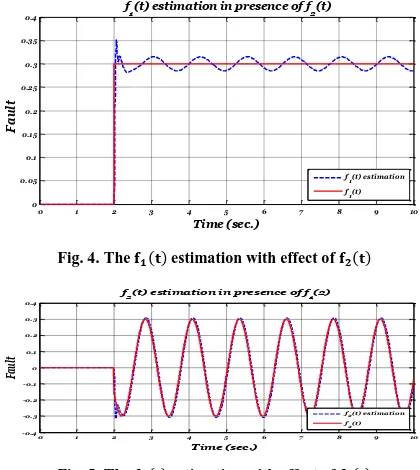
Figs. 4 & 5 show the estimation of the actuator fault signals where both affect the system simultaneously without the presence of the disturbance. It is clear that the proposed algorithm can isolate the effects of simultaneous actuator faults.
Fig. 4.The 𝐟𝟏(𝐭) estimation with effect of 𝐟𝟐(𝐭)
Fig. 5.The 𝐟𝟐(𝐭) estimation with effect of 𝐟𝟏(𝐭)
On the other hand, Figs. 6 & 7 repeat the results shown in Figs. 4 & 5 under the effect of the disturbance on both faults separately.
Fig. 6.The 𝐟𝟏(𝐭) estimation with effect of 𝐝(𝐭)
Fig. 7.The 𝐟𝟐(𝐭) estimation with effect of 𝐝(𝐭)
0 1 2 3 4 5 6 7 8 9 10
-0.5 -0.4 -0.3 -0.2 -0.1 0 0.1 0.2 0.3 0.4 0.5
External disturbance
Time (sec.)
D
is
tur
b
a
n
ce
0 1 2 3 4 5 6 7 8 9 10
0 0.05 0.1 0.15 0.2 0.25 0.3 0.35
Actuator fault f1(t)
Time (sec.)
Fa
ul
t
f1(t) estim ation f1(t)
0 1 2 3 4 5 6 7 8 9 10
-0.4 -0.3 -0.2 -0.1 0 0.1 0.2 0.3
0.4 Actuator fault f2(t)
Time (sec.)
F
a
ul
t
f2(t) estimation
f2(t)
0 1 2 3 4 5 6 7 8 9 10
0 0.05 0.1 0.15 0.2 0.25 0.3 0.35
0.4 f1(t) estimation in presence of f2(t)
Time (sec.)
F
a
ul
t
f1(t) estimation
f1(t)
0 1 2 3 4 5 6 7 8 9 10
-0.4 -0.3 -0.2 -0.1 0 0.1 0.2 0.3 0.4
f2(t) estimation in presence of f1(2)
Time (sec.)
Fa
ul
t
f2(t) es timation
f2(t)
0 1 2 3 4 5 6 7 8 9 10
-0.05 0 0.05 0.1 0.15 0.2 0.25 0.3 0.35 0.4
f
1(t) estimation in presence of d(t)
Time (sec.)
Fa
ul
t
f1(t) estimation f1(t)
0 1 2 3 4 5 6 7 8 9 10
-0.4 -0.3 -0.2 -0.1 0 0.1 0.2 0.3 0.4
f2(t) estimation in presence of d(t)
Time (sec.)
Fa
ul
t
5. CONCLUSIONS
In this paper, a new LMI formulation for robust observer-based FAFE was proposed. The proposed algorithm offers a relaxed LMI design constraint via obviating the need for incorporating the equality constraint. Moreover, the robustness against external disturbances has been considered through the attenuation of the L2norm of the exogenous inputs on the estimation
error. Furthermore, the use of different gains for the proportional and integral terms in the fault estimator dynamics provides freedom in determining a solution to the design problem for a wide range of tuning parameters.
Obviously, fault estimation methods offer great advantages compared with classical residual based FDD methods. This is because fault estimation provides more information such as fault time behaviour, fault severity, and the possibility of using the estimation to compensate for fault effects within the closed-loop system. On the other hand, owing to the importance of the fault estimation accuracy for FDD and FTC, the observer-based fault estimator design must take into account the effects of fault time varying behaviour and the disturbance.
REFERENCES
[1] S. Qikun, J. Bin, S. Peng, and L. Cheng-Chew, "Novel Neural Networks-Based Fault Tolerant Control Scheme With Fault Alarm," IEEE Trans. on Cybernetics, vol. 44, no. 11, pp. 2190-2201, 2014.
[2] L. Ming, C. Xibin, and S. Peng, "Fuzzy-Model-Based Fault-Tolerant Design for Nonlinear Stochastic Systems Against Simultaneous Sensor and Actuator Faults," IEEE Trans. on Fuzzy Systems, vol. 21, no. 5, pp. 789-799, 2013.
[3] T. Jain, J. J. Yame, and D. Sauter, "A Novel Approach to Real-Time Fault Accommodation in NREL's 5-MW Wind Turbine Systems," IEEE Trans. on Sustainable Energy, vol. 4, no. 4, pp. 1082-1090, 2013.
[4] M. Sami and R. J. Patton, "Active sensor fault tolerant output feedback tracking control for wind turbine systems via T–S model," Engineering Applications of Artificial Intelligence, vol. 34, no. 0, pp. 1-12, 2014.
[5] M. Sami and R. J. Patton, "Active Fault Tolerant Control for Nonlinear Systems with Simultaneous Actuator and Sensor Faults," Int. J. of Control, Automation, and Systems, vol. 11, no. 6, pp. 1149-1161, 2013.
[6] R. J. Patton, L. Chen, and S. Klinkhieo, "An LPV pole-placement approach to friction compensation
as an FTC problem," Int. J. Appl. Math. Comput. Sci., vol. 22, no. 1, pp. 149–160, 2012.
[7] H. Alwi, C. Edwards, and A. Marcos, "Fault reconstruction using a LPV sliding mode observer for a class of LPV systems," J. of the Franklin Institute, vol. 349, no. 2, pp. 510-530, 2012.
[8] X. Wei and M. Verhaegen, "Sensor and actuator fault diagnosis for wind turbine systems by using robust observer and filter," Wind Energy, vol. 14, no. 4, pp. 491-516, 2011.
[9] M. Sami and R. J. Patton, "Global wind turbine FTC via T-S fuzzy modelling and control," 8th IFAC Symposium on Fault Detection, Supervision and Safety of Technical Processes, Mexico City, Mexico, 29-31 Aug 2012.
[10] M. Sami and R. J. Patton, "An FTC approach to wind turbine power maximisation via T-S fuzzy modelling and control," 8th IFAC Symposium on Fault Detection, Supervision and Safety of Technical Processes, Mexico City, Mexico, 29-31 Aug 2012.
[11] L. Zhang and A. Q. Huang, "Model-based fault detection of hybrid fuel cell and photovoltaic direct current power sources," J. of Power Sources, vol. 196, no. 11, pp. 5197-5204, 2011.
[12] K. Zhang, B. Jiang, and V. Cocquempot,
"Adaptive Observer-based Fast Fault Estimation," Int. J. of Control, Automation, & Systems, vol. 6, no. 3, pp. 320-326, June 2008.
[13] B. Jiang, K. Zhang, and P. Shi, "Integrated Fault Estimation and Accommodation Design for Discrete-Time Takagi-Sugeno Fuzzy Systems With Actuator Faults," IEEE Trans. on Fuzzy Systems, vol. 19, no. 2, pp. 291-304, 2011.
[14] M. Sami and R. J. Patton, "A Fault Tolerant Control Approach to Sustainable Offshore Wind Turbines," in Wind Turbine Control and Monitoring, N. Luo, et al., Eds., ed: Springer, 2014.
[15] K. Tanaka and H. O. Wang, Fuzzy Control
Systems Design and Analysis: A Linear Matrix Inequality Approach: John Wiley, 2001.
[16] M. C. M. Teixeira and S. H. Zak, "Stabilizing controller design for uncertain nonlinear systems using fuzzy models," IEEE Trans. on Fuzzy Systems vol. 7, no. 2, pp. 133-142, 1999.
[17] H. D. Tuan, P. Apkarian, T. Narikiyo, and Y.
Yamamoto, "Parameterized linear matrix
[18] M. Corless and J. A. Y. Tu, "State and Input Estimation for a Class of Uncertain Systems," Automatica, vol. 34, no. 6, pp. 757-764, 1998.
[19] S. X. Ding, Model-based Fault Diagnosis
Techniques Design Schemes, Algorithms, and Tools: Springer-Verlag, 2008.
[20] T. M. Guerra, A. Kruszewski, L. Vermeiren, and H. Tirmant, "Conditions of output stabilization for nonlinear models in the Takagi-Sugeno's form," Fuzzy Sets and Systems, vol. 157, no. 9, pp. 1248-1259, 2006.