Markovian Delay Prediction-Based Control of Networked
Systems
Behrooz Rahmani i ; and Amir H.D. Markaziii
Received 13February 2008; received in revised 2March 2009; accepted 10 May 2009
i B. Rahmani is PhD Candidate of Mechanical Engineering at Iran University of Science and Technology, Tehran, Iran (e-mail:
ii Corresponding Author, Amir H.D. Markazi is with the Iran University of Science and Technology, Tehran, Iran (e-mail: [email protected]).
ABSTRACT
A new Markov-based method for real time prediction of network transmission time delays is introduced. The method considers a Multi-Layer Perceptron (MLP) neural model for the transmission network, where the number of neurons in the input layer is minimized so that the required calculations are reduced and the method can be implemented in the real-time. For this purpose, the Markov process order is estimated offline, using pr-recorded network time delay history. Unlike most of the previously existing methods, the proposed approach is both accurate and fast enough for a real time implementation. Using such a scheme for real-time estimation of the upcoming time delays, a variable state feedback gain control scheme is also proposed and applied to the predicted discretized model of the plant. The proposed approach is shown, through well-known benchmark problems, to be both accurate and fast enough for a real time implementation.
KEYWORDS
Neural Network, Delay Prediction, Entropy, Markov Order Estimation, Networked Control Systems (NCS), Variable Controller Design
1. INTRODUCTION
A feedback control system in which a control loop is closed through a real-time network is called a networked control system (NCS). In such systems, the controller communicates with sensors and actuators through a network media and the system information, e.g., the reference input, the plant measured output and the control input, is transmitted through the network [1], [2].
A network can be considered as a web of uncertain transmission paths. An important issue, which is the main objective of this paper, is the real time prediction of the network-induced time delay. Such delays affect the control loop from two aspects: 1) the performance degradation; i.e., higher overshoot, larger settling time, etc., and 2) the reduced stability or total instability of the closed-loop system [3]. Such delays can be constant or variable depending on the network type.
The effects of fixed sampling periods on the stability of an NCS, is studied in [2], [4], [5], [6], [7] and [8], and bounds on the transmission delay are found such that the closed loop stability is guaranteed. More recent studies considered the control schemes with variable sampling periods by considering the time delay as the varying sampling period at each step [9]. As a pre-requisite for employing variable sampling schemes, the network delay
pattern must be known or predicted. One approach is to consider the network time delay as a Markov chain [9], [10]. In order to predict such randomly occurring network time delays, Artificial Neural Network theory is employed in [9], [11] and [12], yet the proposed method is not suitable for real-time implementation. In this method, the delay is assumed as a Markov process and the upcoming delay is assumed as a nonlinear function of previous delays.
A real time implementation of such delay prediction methods depends on the amount of required real time calculations. For this purpose, a method for determination of the Markov order is presented in this paper, so that by considering the delay as a Markov chain, only a certain length of previously occurring delays can be used in the predictor, and the required calculations could be minimized without losing the accuracy. Therefore, the proposed method involves two contributions compared to the previous related works. The first contribution is in the proposition of an algorithm for real time prediction of network delay, and second one is in the Markov order estimation, which reduces the required online calculations, without compromising the accuracy of the prediction.
delay is 1) a Markov chain, i.e., it can be essentially predicted based on the previously occurred time delays, 2) is bounded, 3) is Gaussian [13], and 4) is a weekly stationary process. 5) The networks packet loss is not considered.
In the sequel, some discussion about a Markov process and its order estimation is provided, and some relevant results from the neural network methodology are discussed shortly. Then, the proposed algorithm for prediction of the network delay is developed. Moreover, a novel control algorithm is proposed for such systems working based on these predicted delays. Finally, the performance of the prediction and control algorithms are shown by practical simulation studies.
2. MARKOV PROCESS
A Markov chain of order L (or a Markov chain with memory length L) is defined when
)
,
,...
,
(
)
,...,
,
(
x
nx
nx
nx
p
x
nx
nx
nx
nLp
−1 −2 0=
−1 −2 − (1)for all n [15] , [16]. Here, p(|), denotes the conditional probability density function and the set
{
,xn,xn−1,xn−2, ,x1,x0,x−1,x−2,}
is considered as a discrete random process. Estimation of the order of such random process means to find the memory length of the process, L, such that the above conditional probability density functions do not change significantly as L is increased. In the following section a method for estimating the order of a Markov process is discussed.A. Markov Order Estimation
In this section based on the idea first proposed in [17], a measure for the memory length of a Gaussian random process is derived, which turns out to be a simple and effective metric for the purpose of Markov order estimation. As mentioned previously, the order of a Markov process can be determined by finding L such that the conditional probability density function, right hand of Equation 1, does not change significantly as L is increased [15], [16], [17] and [18]. One measure of this change is the Kullback-Leibler divergence that measures the distance between two probability density functions; i.e., the distance between both sides of Equation 1. Such a metric can be considered as a performance index that shows the accuracy of approximating a Gaussian random process by an L-th order Markov chain. Since, often, the left hand side of Equation 1 is not available, the distance between p(xnxn−1,xn−2,...,xn−L)and p(xnxn−1) can be defined as [17]
L n n n n n L n n n n L n n n n dx dx dx x x p x x x x p x x x x p d − − − − − − − − − × = ... ) ( ) , ,... , ( log ) ,..., , , ( 1 1 2 1 2 1 (2)
Using the Bayesian theorem, Equation 2 can be written as
L n n n n L n n n n n L n n n L n n n n dx dx dx x x x p x x p x x x x p x x x x p d − − − − − − − − − − − − = ... ) ,..., ( ) ( ) ,..., , ( log ) ,..., , , ( 1 1 2 1 1 2 2 1 (3)
which is equal to the mutual information between the present sample, xn, and the L-1 samples prior to the immediate previous sample, xn, provided that the immediate previous sample is available, i.e.,
)
,...,
,
;
(
−2 −3 − −1=
I
x
nx
nx
nx
nLx
nd
. (4)This value can be normalized by unconditional mutual information,I(xn;xn−1,xn−2,xn−3,...,xn−L). The obtained value can be considered as the discrepancy between the first and the L-th order conditional probability density functions of a random process, i.e.,
) ,..., , , ; ( ) ,..., , ; ( ) ,..., , , ; ( L n n n n n n L n n n n L n n n n n x x x x x I x x x x x I x x x x x I d D − − − − − − − − − − − − = = 3 2 1 1 3 2 3 2 1
. (5)
Also it can be proved that [18]
)
;
(
)
,...,
,
,
;
(
)
,...,
,
;
(
1 3 2 1 1 3 2 − − − − − − − − −−
=
n n L n n n n n n L n n n nx
x
I
x
x
x
x
x
I
x
x
x
x
x
I
(6) then, ) ,..., , , ; ( ) ; ( L n n n n n n n x x x x x I x x I D − − − − − − = 3 2 1 1 1 (7)Equation 7 represents the relative information loss due to the approximation of the process by a first order Markov process compared to that of the L-th order ones. Then it can be used as an index for estimating the order of a Markov process: converging D as L is increased shows that the mutual information between the present symbol and the symbols prior to L-1 are negligible; in other words, these symbols do not have any information about the present symbol. Therefore, the order of the discussed Markov process is L. In the following section, this formula is applied to a Gaussian random process and a simple formula is derived for this case.
B. Gaussian Random Process Implementation
For a Gaussian, zero-mean, random process, the joint probability density function, is given by [16]
− = − X C X C x
p T n
n n X 1 2 1 exp ) det( ) 2 ( 1 ) ( π (8)
where,X =
[
x1 x2 ... xn]
; T denotes the matrix transpose and Cn is the n×ncovariance matrix of X.It is well known [18] that the mutual information,
) , (x y
) , ( ) ( ) ( ) ( ) ( ) ,
(x y H x H xy H x H y H x y
I = − = + − (9)
where H(x) is the differential entropy ([15] and [16]), which for a Gaussian process is equal to
) , 1 ( 3 2
1 ln(2 )
2 1 ) ,..., , ,
( n n L
L L
n n n
n x x x e
x
H − − − − = π ∆ − − (10)
Then, ) ,..., , , ( ) ,..., , ( ) ( ) ,..., , , ; ( 2 1 2 1 3 2 1 L n n n n L n n n n L n n n n n x x x x H x x x H x H x x x x x I − − − − − − − − − − − + = (11) That is, ) , ( 1 ) , 1 ( 2 3 2 1 ) 2 ln( 2 1 ) 2 ln( 2 1 2 ln 2 1 ) ,..., , , ; ( L n n L L n n L L n n n n n e e e x x x x x I − + − − − − − − ∆ − ∆ + = π π π σ (12)
where ∆(n−1,n−L)=det(cov(xn−1,...,xn−L)) and )) ,..., , det(cov( 1 ) ,
(nn−L = xn xn− xn−L
∆ . Finally, Equation 12
can be written as
∆ ∆ = − − − − − − − ) , ( ) , 1 ( 2 3 2 1 ln 2 1 ) ,..., , , ; ( L n n L n n L n n n n
n x x x x
x
I
σ
(13)and ∆ = − − ) 1 , ( 4 1 ln 2 1 ) ; ( n n n n x x
I
σ
(14)Equation 7 can now be simplified as
∆ ∆ ∆ − = − − − − ) , ( ) , 1 ( 2 ) 1 , ( 4 ln ln 1 L n n L n n n n D
σ
σ
(15)Equation 15 can be employed to determine the order of the delay as a Markov chain, L. For this reason, the obtained delay time history is assumed to be Gaussian and it is shifted such that its mean becomes zero. After that, Equation 15 is utilized to calculate D, and, hence, the order of the Markov process is determined, such that by increasing L, D increases only slightly.
3. THE PROPOSED NETWORK DELAY PREDICTOR
Network delay prediction can be performed using various neural network supervising models, such as a Feed-Forward, multi layer perceptron (MLP) neural network. In this paper, the focus is on the Levenberg-Marquardt algorithm that is a Hessian-based algorithm for nonlinear least squares optimization [14]. It is one of the most accurate algorithms for function approximation problems. In this section, the proposed delay predictor is developed.
A. Neural Network Delay Predictor
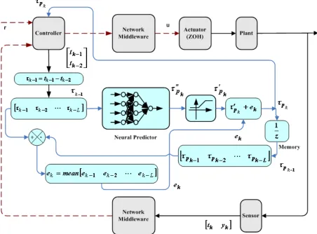
Neglecting the measurement time delay, the sum of the sensor-to-controller and controller-to-actuator time delays can be considered as the total instantaneous time delay of the network. Such a time delay can be computed using the time stamp attached to the signal, which is received by the actuator at every sampling instant. Suppose that the sampled output of the plant is sent at time K0, and received by the actuator at K0+
τ
sc+τ
ca, whereτ
sc andca
τ
denote the network feedback and forward time delays, respectively. Neglecting the computational time delay, the total time delay of the loop can be calculated by comparing such time values. The prediction procedure is carried out in two steps: first, a neural network model comprised of L inputs, one hidden layer of L neurons and one output layer with one neuron is devised, as the primary delay predictor (Figure 2). In this scheme, the current delay is assumed to be a nonlinear function of L previous delays, where, L is estimated as proposed in the previous section. Due to possible large changes in the network traffic condition, the time delay prediction made by this model may involve some errors. To overcome such a difficulty, a neural network modifier is utilized, in which the expected bounds on the time delay, obtained from the network delay history, is decided.This prediction procedure can be summarized as follows:
1.The delay time history of a typical network is obtained by offline observations; in a TCP/IP network, e.g., this can be obtained by using the
"ping" command between the two internet nodes. 2.Expected upper and lower bounds on the network
delay are calculated from the history.
3.The procedure of Section 2 is employed to determine the order of the delay, L, assuming a Markov chain. 4.The proposed neural network MLP model is
initialized, i.e., initial values for weights and biases are assigned.
5.The neural predictor is trained offline using the Levenberg-Marquardt algorithm.
6.Using the L most recent time delays the next upcoming time delay is estimated.
7.If the predicted delay turns out to be larger/smaller than the upper/lower bounds, respectively, it is replaced by the corresponding bound.
8.This actual value of the current delay is compared with the predicted one and the difference is included as the L-th entry of the vector of the L recent prediction errors, and the next prediction error is assumed to be the average of the entries of this vector.
9.The upcoming estimated delay is modified by adding the predicted error to the predicted delay.
variations are bounded, Gaussian and weekly stationary, then a rather accurate prediction can be expected.
4. VARIABLE SAMPLING PERIOD CONTROL
SCHEME
While, in a high bandwidth network, it is possible to implement a discrete-time control system using a fixed continuous-time state feedback gain, yet this may not be useful when the network traffic is high and a sufficiently fast sampling may not be guaranteed. The rationale behind the variable sampling control scheme can be stated as follows: Suppose, at the outset of every sampling instant, the upcoming network delay can be predicted approximately. Then, it makes sense to select the next sampling period equal to the predicted time delay. By discretizing the continuous time model of the plant, a suitable controller, e.g., a state feedback gain, can then be designed for application during the next sampling interval.
It must be noted that, with a state feedback controller, which is a memory-less controller, the sensor-to-controller and the sensor-to-controller-to-actuator time delays have the same effects on the control loop, hence, they can be added up, and compensated by an overall time advance in the control algorithm. For this purpose, the network time delay prediction method proposed in Section 3, can be used for an estimation of the required time advance in issuing the control input for the plant. In the following, a novel control method is proposed which can tangibly compensate the instability due to the network delay.
A. Modeling and Control Methodology
Consider a continuous-time model of a multi-input multi-output (MIMO), linear time-invariant system with a constant time delay,
τ
, i.e.,(16)
( ) ( ) ( )
x t =A x t +Bu t−τ
,
y =Cx
where xt Rn
∈
)
( , m
R t
u()∈ , l
R t
y()∈ , nn
R
A∈ × , B∈Rn×m,
and C∈Rl×n. The time response for the discrete-time
model of this system, during the k-th sampling interval can be expressed as [19]
(17) 0
( ) A T ( ) T A ( )
x kT T e x kT e ηBu kT T η τ dη
+ = + + − −
It can be shown that if the delay is larger than one sampling period, the value of states depends on the several recent weighted inputs, and the control problem becomes more difficult.
Here, a new simplifying approach, in the case of large delay for modeling of an NCS is proposed. It is devised that at the outset of the k-th sampling instant, the next sampling period is set equal to the predicted time delay, i.e., Tk=τ. Such an assumption becomes more realistic, when the sensor is assumed event driven, i.e., where the plant output is sampled only when new data reaches to the actuator. For this case, it can be shown that the discrete model can be simplified as
(18)
1 1,
k k k k k
x+ = Φ x + Γu−
where ATk
k
k =ΦT =e
Φ ( ) and Γ =Γ = Tk A
k
k T e Bd
0 )
( η η
Using the assumption of state feedback and zero input disturbance and sensor noise, the next upcoming plants state vector can be predicted:
(19)
1 1 1
1) ( )
(
ˆk =xk =ΦTk− xk− +ΓTk− uk−
x
Clearly, Φkand Γkdepend on Tk; hence, the control
input,
u
k , at the k-th sampling instant, can be updatedaccording to the following state-feedback law:
(1) k
T k T
k K x K x
u
k
k =−
−
= ˆ
where k
T
K is the controller gain calculated using pole placement or LQR techniques according with the updated sampling period, Tk.
Figure 1. The proposed delay prediction algorithm for networked control systems.
5. NUMERICAL EXAMPLES
A. Example: Evaluating the Neural Based Delay
Predictor
In order to evaluate the effectiveness of the proposed delay prediction algorithm, an internet delay history is captured and used. In this simulation, the ping command was used to obtain the Round Trip Time (RTT) between a PC in our laboratory (at the Iran University of Science and Technology) as the controlled plant and the server of www.google.com as the central controller. RTT is the total time needed to transmit a signal over a network up to a destination and back and can be considered as the total delay time for transmit, receive and service times. Therefore, it is a measure of the total delay of the network in both forward and backward channels, i.e., total delay of the control loop for the illustrated case study. The histogram and the plot of this data are shown in Figure 3 and Figure 4. Using this history, the proposed approach in Section 2 is employed to estimate the order of the network delay as a Markov chain, namely L. As shown in Figure 5, it is evident that the order of the process turns out to be 4. Then, the expected upper and lower bounds on the
network delay were calculated and the proposed neural predictor with the specified number of the input-output neurons was trained offline by the Levenberg-Marquardt algorithm using the MATLAB/Neural Network Toolbox. Then, for each time step, the latest L most recently occurred time delays were used to predict the next upcoming time delay. If the predicted delay turned out to be larger or smaller than the upper or lower bounds, respectively, it is replaced by the corresponding bound obtained previously. After the reception of the next sample by the controller, in the next time instant, the actual value of the occurred delay of the previous sample was computed and was compared with the predicted ones. Therefore, the difference is the prediction error considered as the L-th entry of the vector of the L most recent prediction errors, and the next prediction error was assumed to be the average of the entries of this vector. Finally, the upcoming predicted delay was modified by adding the predicted error to the predicted delay. This procedure was carried out in each sampling period to ensure an accurate prediction.
Using L as the number hidden neurons provides sufficient degree of freedom for the learning process, so that an accurate prediction of the time delay becomes possible. Simulations studies reveal that using less than L number of hidden neurons, reduces the accuracy significantly, while more than L hidden neurons provides insignificant improvement in the final results. Therefore, for minimizing the computation time, while keeping the desired accuracy, L neurons are considered in the hidden layer (Figure 2).
Figure 2. Neural Network model.
Figure 3. Histogram of the delay of a typical communicational network.
Figure 4. Plot of the delay of a typical communicational network vs. data packet number.
Figure 5. Delay order Estimation.
Figure 6. The predicted and real delay vs. data packet number.
Figure 7. Error of the delay prediction algorithm in seconds using the MLP neural model with modifier vs. data packet number.
0 2 4 6 8 10 12 14
10 9 8 7 6 5 4 3 2
number of inputs
P
re
d
ic
ti
o
n
M
e
a
n
E
rr
o
r(
m
s
)
REPA [12] RBF [11] Simple MLP [9] Proposed Method
Figure 8. Mean prediction error with various methods versus the number of inputs.
B. Example: Variable Prediction Based Control
Algorithm
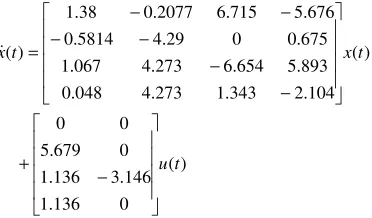
The unstable batch reactor [20] is a coupled two-input, two-output NCS. In the second example, digital networked control of this MIMO plant is discussed:
) (
0 136 . 1
146 . 3 136 . 1
0 679 . 5
0 0
) (
104 . 2 343 . 1 273 . 4 048 . 0
893 . 5 654 . 6 273 . 4 067 . 1
675 . 0 0 29 . 4 5814 . 0
676 . 5 715 . 6 2077 . 0 38 . 1
) (
t u
t x t
x
− +
− −
− −
− −
=
Since the eigenvalues of the systems matrix are
[
1.99 0.064 −5.057 −8.67]
, the reactor is unstable. Assuming an ideal zero-delay network, and using the Linear Quadratic Regulator (LQR) to design the state feedback controller, the response of the continuously closed loop controlled system, and under an initial condition of x0=[
1 −1 0.5 0.5]
T is shown in Figure 9. Now, a network with the delay pattern similar to the pattern shown in Figure 4 is used to transferring the control signals and the proposed control method is applied to this networked system. The closed-loop response of the new system, illustrated in Figure 10, demonstrates the exceptional effectiveness of the proposed algorithm, compared to the ideal response of Figure 9.0 0.5 1 1.5 2 2.5 3 3.5 4 4.5 5
−1 −0.5 0 0.5 1 1.5
Initial State Response: Control Input; Continuous Closed−Loop System
Time (s)
States
x1 x2 x3 x4
Figure 9. Closed-loop response with a fixed control gain through an ideal zero-delay network under an initial condition of
[
]
T5 . 0 5 . 0 1
1 − .
0 0.5 1 1.5 2 2.5 3 3.5 4 4.5 5
−1 −0.5 0 0.5 1 1.5
Time (s)
States
Initial State Response: States
x1 x2 x3 x4
Figure 10. Closed-loop (initial state) response with the proposed variable gain method through a real network under an initial
6. CONCLUSION
In this paper, a novel Markov process based method for real time prediction of the network transmission time delays is proposed. A real time implementation of such delay prediction methods depends on the amount of required real time calculations. For minimizing the calculation time, a method for determination of the delay Markov process order is presented. For this purpose, we have proposed an algorithm for the real time prediction of network delay based on a novel online modifiable neural network scheme, and a method for Markov order estimation, which can reduce the needed calculations for a
better real time implementation possibility. To evaluate the effectiveness of the proposed time prediction algorithm, use was made from realistic data obtained through internet connections. Experiments on the real-time data show that the delay prediction algorithm has enough capability to estimate the upcoming time delays, in the real time. Moreover, the simulation of the MIMO unstable plant reveals the performance of the proposed controller design method.
Acknowledgment: The authors would like to thank the anonymous referees for their constructive suggestions, which improved the content substantially.
7. REFERENCES
[1] T.C. Yang, “Networked control system: a brief survey”, IEE Proc.-Control Theory Appl., Vol. 153, 2006, pp. 403-412.
[2] W. Zhang, M. S. Branicky, and S. M. Phillips, “Stability of Networked Control Systems”, IEEE Control Systems Magazine, 2001, pp. 84-99.
[3] Y. Tipsuwan and M. Y. Chow, “Control methodologies in networked control systems”, Control Engineering Practice 11, 2003, pp. 1099–1111.
[4] C. Ma, S. Chen and W. Liu, “Maximum allowable delay bound of networked control systems with multi-step delay”, Simulation Modeling Practice and Theory, 2007, pp. 513–520.
[5] G. P. Liu, Y. Xia, D. Rees, and W. Hu, “Design and Stability Criteria of Networked Predictive Control Systems With Random Network Delay in the Feedback Channel”, IEEE Transaction on Systems, Vol. 37, No. 2, 2007, pp. 173-184.
[6] L. Zhang, Y. Shi, T. Chen, and B. Huang, “A new method for stabilization of networked control systems with random delays”, IEEE Transaction on Automatic Control, 2005, pp. 1177–1181. [7] L. Zhang and F. Huajing, “A novel controller design and
evaluation for networked control systems with time-variant delays”, Journal of the Franklin Institute, (2006), pp. 161–167. [8] L. Zhang and F. Huajing, “Fuzzy controller design for networked
control system with time-variant delays”, Journal of Systems Engineering and Electronics, Vol.17, No. 1, 2006, pp.172– 176. [9] J. Yi, Q. Wang, D. Zhao and J. T. Wen, “BP neural network
prediction-based variable-period sampling approach for networked control systems”, Applied Mathematics and Computation, 2006, pp. 976–988.
[10] Zhang, L., Shi, Y., Chen, T., and Huang, B., “A new method for stabilization of networked control systems with random delays, IEEE TRANSACTIONS ON AUTOMATIC CONTROL, Vol. 50, 2005, pp. 1177–1181.
[11] Q.P. Wang, D.L. Tan, Ning Xi, Y.C. Wang, “The Control Oriented QoS: Analysis and Prediction”, Proceedings of the 2001, IEEE International Conference on Robotics 8 Automation.
[12] North, S. Sahin, F., "Picasso: real-time estimation of network delay over a tele-robotic link", IEEE International Conference on Systems, Man and Cybernetics, 2002.
[13] S. Soucek and G. koler, “Impact of QOS parameter on Internet-Based EIA-709.1 Control Applications”, IEEE Conference Proceeding, USA, Vol. 4, 2002, pp. 3176-3181.
[14] N. N. R. Ranga Suri, D. Deodhare and P. Nagabhushan, “Parallel Levenberg -Marquardt-based Neural Network Training on Linux Clusters - A Case Study”, Proceedings of the Third Indian Conference on Computer Vision, Graphics & Image Processing, India, 2002.
[15] S. Miller and D. Childers, Probability and Random Processes: With Applications to Signal Processing and Communications, Academic Press, 2004.
[16] S. U. Pillai and A. Papoulis, Probability, Random Variables, and Stochastic Processes, McGraw-Hill, 2002.
[17] H. Kong and E. Shwedyk, “A Measure for the Length of Probabilistic Dependence”, IEEE, ISlT, Ulm, Germany, 1997, pp. 469.
[18] T. M. Cover and J. A. Thomas, Elements of Information Theory, Wiley-Interscience, 1991.
[19] K. J. Astrom (Author), and B. Wittenmark, Computer-Controlled Systems: Theory and Design, Prentice Hall; 3 edition, Nov 20 1996.