The importance of increasing returns to scale in the process of agglomeration in Portugal: A non linear empirical analysis

(1)

The importance of increasing returns to

scale in the process of agglomeration in

Portugal: A non linear empirical analysis

Martinho, Vítor João Pereira Domingues

Escola Superior Agrária, Instituto Politécnico de Viseu

2011

Online at

https://mpra.ub.uni-muenchen.de/32204/

(2)

THE IMPORTANCE OF INCREASING RETURNS TO SCALE IN THE PROCESS

OF AGGLOMERATION IN PORTUGAL: A NON LINEAR EMPIRICAL ANALYSIS

Vitor João Pereira Domingues Martinho

Unidade de I&D do Instituto Politécnico de Viseu Av. Cor. José Maria Vale de Andrade

Campus Politécnico 3504 - 510 Viseu

(PORTUGAL)

e-mail: [email protected]

ABSTRACT

With this work we try to analyse the agglomeration process in the Portuguese regions, using the New Economic Geography models. In these models the base idea is that where has increasing returns to scale in the manufactured industry and low transport costs, there is agglomeration. Of referring, as summary conclusion, that with this work the existence of increasing returns to scale and low transport cost, in the Portuguese regions, was proven and as such the existence of agglomeration in Portugal.

Keywords: new economic geography; non linear models; Portuguese regions.

1. INTRODUCTION

With this study we mainly aimed to analyze the process of agglomeration across regions (NUTS II and NUTS III) of Portugal, using non linear models of New Economic Geography, in particular, developments considered by (1)Krugman (1991), (2)Thomas (1997), (3)Hanson (1998) and (4)Fujita et al. (2000). We will also try to compare the results obtained by the empirical models developed by each of these authors.

(3)

with characteristics cumulative. The work developed at the level of economic geography, traditional and recent attempt to explain the location of economic activities based on spatial factors. The liberal economic policies, international economic integration and technological progress have created, however, new challenges that promote agglomeration (7)(Jovanovic, 2000). So, have been developed new tools for economic geography, such as increasing returns, productive linkages, the multiple equilibria (with the centripetal forces in favor of agglomeration and centrifugal against agglomeration) and imperfect competition. These contributions have allowed some innovations in modeling the processes of agglomeration, which has become treatable by economists, a large number of issues. In particular the inclusion of increasing returns in the analytical models, which led to the call of increasing returns revolution in economics (Fujita et al., 2000). (8-10)Krugman (1994, 1995 and 1998) has been the central figure in these developments. (11)Fujita (1988),(12) Fujita et al. (1996) and (13)Venables (1996), in turn, have been leaders in the development and exploration of the implications of economic models of location, based on increasing returns. These developments have helped to explain the clustering and "clustering" of companies and industries.

Hanson, in 1998, taking into account the model of Krugman (1991) and the extent of Thomas (1997) this model, had a good theoretical and empirical contribution to empirically examine, with reduced forms, the relationship between increasing returns to scale, costs transportation and geographical concentration of economic activity.

2. THE MODEL

The model of Krugman (1991) describes himself, then, as follows:

i i i

i w

Y (1)  , income equation (1)

i e

w G

j

d j j i

ij 

   

 





 

, )

(

1 1 1 



 , índex price equation (2)

i e

G Y w

j

d j j i

ij 

   

 





 

, ) (

1 1 

 

, nominal wage equation (3)



        

j i j

i

G G w

w

(4)

In these equations, Yi is the income in region i, wi the wage in region i, _i is the percentage of agricultural workers in region i, Gi the price index for manufactured goods in the region i and dij is the distance between each pair of locations. In equilibrium the region i share _i employed in sector of manufactured goods which is equal to the fraction of companies located in manufactured goods in region i, ni/n. Alternatively Thomas (1997) presents the following extension of the model of Krugman (1991):

i i i Lw

Y  , i, income equation (5)

i i

iH Y

P (1) , i, housing price equation (6)

i e

w G

j

d j j i

ij 

   

 





 

, )

(

1 1 1 



 , price índex equation (7)

i e

G Y w

j

d j j i

ij 

   

 





 

, ) (

1 1 

 

nominal wage equation (8)

  



j j

j i

i i

G P

w

G P

w

   1

1 , i j, real wage equation (9)

Yi is the income in region i, wi the wage in region i, L the total supply of workers for the manufactured goods sector, _i the percentage of employees in the sector of manufactured products, Pi the price of housing in region i, the Gi price index for manufactured goods in region i, Hi the supply of housing in the region i and dij is the distance between each pair of locations.

Recently Fujita et al. (2000) also presented an alternative model:

i i

i

i w

Y  (1) , income equation (10)

) 1 /( 1 1

) (

  

 

   

  



j

ji j j

i w T

G , price equation (11)

  

/ 1 1 1

   

 





 

j

j ij j i Y T G

(5)

  _ 

i i

i wG , real wage equation (13)

Yi is the income in region i, wi the wage in region i, _i is the percentage of agricultural workers in the region i, _i the percentage of employees in the sector of manufactured products, Gi price index for manufactured goods in region i, and Tij transport costs between regions i and j.

The parameters to be estimated, these models are  the elasticity of substitution between manufactured goods,  the share of expenditure on manufactured goods and  the transport costs to send a unit of manufactured goods in a unit distance.

Note that, as can be seen, the three models are very similar, the main difference is that Thomas (1997) have considered building housing sector (power anti-agglomeration) and have created more than one equation and Fujita et al . (2000) have considered transport costs as variables and not considered as parameters in their models Krugman (1991) and Thomas (1997).

It should be noted also that the equations of the income of the previous models, it is assumed that agricultural workers earn the same wage everywhere, given that agricultural goods are freely transported. Were chosen, on the other hand, units such that there are  workers in manufacturing and ₁__ agricultural workers.

It could be argued that as industrial workers who are potential users, then locations with large concentrations also tend to have high demand for manufactured goods. This concentration of consumers and producers to some extent explains the cumulative process that may lead to agglomeration phenomena.

Following procedures of Hanson (1998), substituting equations (1) and (4) in (2) yields the reduced equation (14), substituting equations (5), (6) and (9) in (8) obtain the reduced equation (15) and substituting equations (10) and (13) in (11) yields the reduced equation 16, namely:

i j

d j

j i

ij

e w Y C

w    



     

   





 



 ( 1)

1 1

log )

log( , (14)





        

j

i d j

j j

i

ij

e w H

Y D

w    

 

  

 

) log(

)

log( ( 1)

1 ) 1 )( 1 ( 1 ) 1 ( 1

(6)

i j

ij j j

i F Y w T

w    

           



  

 ( 1)

1 1

log )

log( , (16)

Thus Hanson (1998a) solved the problem of lack of price indices for manufactured products and prices for housing at more disaggregated geographic levels. In the last two equations C, D and F are constants and parameters, and _i, _i and _i are error terms.

Furthermore, if the sources of correlation are unobservable factors that are constant over time, then these factors can be controlled using a specification with differentiation in time, which makes the variables expressed in growth rates. Given the dearth of statistical data for the Portuguese regions and the small size of the Portuguese territory, this third alternative to solve the problems of endogeneity seems to be the most viable and as such will be adopted in this work.

Using the differences in the timing of the regression equations, the equation (14) becomes: it j d jt jt j d jt jt it ij ij e w Y e w Y

w  

                          



         ) log( ) log( ) log( ) 1 ( 1 1 1 ) 1 ( 1 1 , (17)

Equation (15) is also:

it j d jt jt jt j d jt jt jt it ij ij e w H Y e w H Y

w  

                                      



                  ) log( ) log( ) log( ) 1 ( 1 1 ) 1 )( 1 ( 1 1 ) 1 ( 1 ) 1 ( 1 ) 1 )( 1 ( 1 ) 1 ( 1 , (18)

(7)

it

j

ijt jt jt j

ijt jt jt it

T w Y

w  

 

   

 

    

 

    

 

 





     

  



) log(

) 1 ( 1 1 1 1

) 1 ( 1

1

(19)

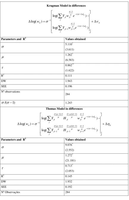
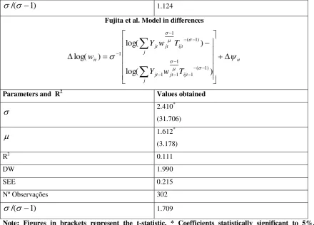
On balance, taking into account the developments of the New Economic Geography, a value /( 1) greater than one indicates that the production is subject to increasing returns to scale. This is because, for the New Economic Geography economies of scale arise through the number of varieties of manufactured goods will be greater the lower the elasticity of substitution  . Thus, the lower the elasticity of substitution is further away from one the value of /( 1) and the greater the increasing returns to scale.

(14)Krugman (1992) shows that if (1)1, then increasing returns to scale are sufficiently weak or the fraction of the manufactured goods sector is sufficiently low and the range of possible equilibria depends on transport costs. If (1)1, then increasing returns are sufficiently strong or the fraction is sufficiently high, such as economic activity is concentrated geographically to any value  .

3. THE DATA USED

Considering the variables of the model presented previously, and the availability of statistical information, we used the following data at regional level: temporal data from 1987 to 1994 for the five regions (NUTS II) in mainland Portugal and for the various manufacturing industries existing in these regions, from the regional database of Eurostat statistics (Eurostat Regio of Statistics 2000), and data for the period 1995 to 1999, for the five regions and for total manufacturing, from the INE (National Accounts 2003).

4. ESTIMATIONS MADE

(8)

forces of anti-agglomeration by immobile factors. Anyway, the point that it confirms the results obtained with the estimates of three equations of some importance, but small, transport costs, given the low values of the parameter  . Looking at the increasing returns to scale, calculating, as noted, the value  /(1), it appears that this is always greater than one, reflecting the fact that there were increasing returns in the Portuguese regions in this period. It should be noted also that the parameter values  are unreasonably high in all three estimations, however, as stated (15)Head et al. (2003) there is a tendency for these values fall around the unit in most empirical work.

(9)

[image:9.595.67.502.107.777.2]

Table 1: Results of estimations of the models of Krugman, Thomas and Fujita et al., in temporal differences, for the period 1987-1994, with panel data (at NUTS II level)

Krugman Model in differences

it j d jt jt j d jt jt it ij ij e w Y e w Y

w  

                          



         ) log( ) log( ) log( ) 1 ( 1 1 1 ) 1 ( 1 1

Parameters and R2 Values obtained

 5.110*

(3.611)

 1.262*

(6.583)

 0.862**

(1.622)

R2 0.111

DW 1.943

SEE 0.196

Nº observations 284 ) 1 /(   1.243

Thomas Model in differences

w  

                                      



                  ) log( ) log( ) log( ) 1 ( 1 1 ) 1 )( 1 ( 1 1 ) 1 ( 1 ) 1 ( 1 ) 1 )( 1 ( 1 ) 1 ( 1

 9.076*

(2.552)

 1.272*

(21.181)

 0.713*

(2.053)

R2 0.145

DW 1.932

SEE 0.192

(10)

) 1 /( 

 1.124

Fujita et al. Model in differences

it j ijt jt jt j ijt jt jt it T w Y T w Y

w  

                        



          ) log( ) log( ) log( ) 1 ( 1 1 1 1 ) 1 ( 1 1

 2.410*

(31.706)

 1.612*

(3.178)

R2 0.111

DW 1.990

SEE 0.215

Nº Observações 302

) 1 /( 

 1.709

[image:10.595.67.508.71.387.2]

Note: Figures in brackets represent the t-statistic. * Coefficients statistically significant to 5%. ** Coefficient statistically significant 10%.

Table 2: Results of estimations of the models of Krugman, Thomas and Fujita et al., in

temporal differences, for the period 1995-1999, with panel data (the level of NUTS III) Krugman Model in differences

it j d jt jt j d jt jt it ij ij e w Y e w Y

w  

                          



         ) log( ) log( ) log( ) 1 ( 1 1 1 ) 1 ( 1 1

 7.399**

(1.914)

 1.158*

(15.579)

 0.003

(0.218)

R2 0.199

DW 2.576

(11)

Nº observations 112

) 1 /( 

 1.156

Thomas Model in differences (with agricultural workers to the H)

w  

                                      



                  ) log( ) log( ) log( ) 1 ( 1 1 ) 1 )( 1 ( 1 1 ) 1 ( 1 ) 1 ( 1 ) 1 )( 1 ( 1 ) 1 ( 1

 18.668*

(3.329)

 0.902*

(106.881)

 0.061*

(2.383)

R2 0.201

DW 2.483

SEE 0.023

) 1 /(   1.057 ) 1 ( 

  1.830

Thomas Model in differences (with housing stock to the H)

w  

                                      



                  ) log( ) log( ) log( ) 1 ( 1 1 ) 1 )( 1 ( 1 1 ) 1 ( 1 ) 1 ( 1 ) 1 )( 1 ( 1 ) 1 ( 1

 11.770

(1.205)

 1.221*

(8.993)

 0.003

(0.314)

R2 0.173

DW 2.535

SEE 0.024

(12)

Fujita et al. Model in differences

it

j

ijt jt jt j

ijt jt jt it

T w Y

w  

 

   

 

    

 

    

 

 





     

  



) log(

) 1 ( 1 1 1 1

) 1 ( 1

1

 5.482*

(4.399)

 1.159*

(14.741)

R2 0.177

DW 2.594

SEE 0.023

) 1 /( 

 1.223

Note: Figures in brackets represent the t-statistic. * Coefficients significant to 5%. ** Coefficients significant acct for 10%.

5. CONCLUSIONS

(13)

interaction between these two forces, traces the evolution of the spatial structure of the economy.

Note that the results obtained with the estimates of Thomas model equations are statistically more satisfactory, possibly because they consider these equations in addition to the centrifugal forces present in increasing returns, also by centrifugal forces, in this work, the

number of employees in the sector agricultural.

It should be noted, finally, that transport costs have had some importance in the evolution of the space economy in Portugal, which amount has been decreasing in recent years, which is understandable given the investments that have been made in terms of infrastructure structures, especially after the appointed time our entry into the European Economic Community in 1986, with the support that has been under structural policies.

6. REFERENCES

1. P. Krugman. Increasing Returns and Economic Geography. Journal of Political Economy, 99, 483-499 (1991).

2. A. Thomas. Increasing Returns, Congestion Costs and the Geographic Concentration of Firms. Mimeo, International Monetary Fund, 1997.

3. G. Hanson. Market Potential, Increasing Returns, and Geographic concentration. Working Paper, NBER, Cambridge, 1998.

4. M. Fujita; P. Krugman and J.A. Venables. The Spatial Economy: Cities, Regions, and International Trade. MIT Press, Cambridge, 2000.

5. G. Myrdal. Economic Theory and Under-developed Regions. Duckworth, London, 1957. 6. A. Hirschman. The Strategy of Economic Development. Yale University Press, 1958. 7. M.N. Jovanovic. M. Fujita, P. Krugman, A.J. Venables - The Spatial Economy. Economia Internazionale, Vol. LIII, nº 3, 428-431 (2000).

8. P. Krugman. Complex Landscapes in Economic Geography. The American Economic Review, Vol. 84, nº 2, 412-416 (1994).

9. P. Krugman. Development, Geography, and Economic Theory. MIT Press, Cambridge, 1995.

10. P. Krugman. Space: The Final Frontier. Journal of Economic Perspectives, Vol. 12, nº 2, 161-174 (1998).

(14)

12. M. Fujita and T. Mori. The role of ports in the making of major cities: Self-agglomeration and hub-effect. Journal of Development Economics, 49, 93-120 (1996).

13. A.J. Venables. Equilibrium locations of vertically linked industries. International Economic Review, 37, 341-359 (1996).

14. P. Krugman. A Dynamic Spatial Model. Working Paper, NBER, Cambridge, 1992.