New Adaptive UKF Algorithm to Improve the Accuracy of SLAM

* Corresponding author address: Yazd University, Yazd, Iran,

Tel.: +98-35-31232495; fax: +98-35-38212781., E-mail address: [email protected].

A

New Adaptive UKF Algorithm to Improve the

Accuracy of SLAM

Masoud S. Bahraini

a,b

, Mohammad Bozorg

a,*

, Ahmad B. Rad

b a _{Department of Mechanical Engineering, Yazd University, Yazd, Iran, P.O. Box, 89195-741}

b _{School of Mechatronic Systems Engineering, Simon Fraser University, Surrey, BC V3T 0A3, Canada}

A R T I C L E I N F O _{A B S T R A C T}

Article history: Received: 26 June, 2017

Received in revised form:

15 January, 2018

Accepted: 30 June, 2018

SLAM (Simultaneous Localization and Mapping) is a fundamental problem when an autonomous mobile robot explores an unknown environment by constructing/updating the environment map and localizing itself in this built map. The all-important problem of SLAM is revisited in this paper and a solution based on Adaptive Unscented Kalman Filter (AUKF) is presented. We will explain the detailed algorithm and demonstrate that the estimation error is significantly reduced and the accuracy of thenavigation is improved. A comparison among AUKF, Unscented Kalman Filter (UKF) and Extended Kalman Filter (EKF) algorithms is investigated through simulated as well as experimental dataset. An indoor dataset is generated from a two-wheel differential mobile robot in order to validate the robustness of AUKF-SLAM to noise of modeling and observation, and to examine the applicability of the method for real-time navigation. Both experimental and simulation results illustrate that AUKF-SLAM is more accurate than the standard UKF-SLAM and the EKF-SLAM. Finally, the well-known Victoria Park dataset is used to prove the applicability of the AUKF algorithm in large-scale environments.

Keywords: SLAM Adaptive UKF Scaling Parameter Mobile Robots

1. Introduction

SLAM is regarded as an essential attribute of an autonomous robot whereby the robot position and its pose are concurrently estimated. Many navigation functions such as goal determination and motion planning depend on successful solution of the SLAM problem. The problem has been extensively addressed via probability based approaches in particular Extended Kalman filter (EKF). Guivant and Nebot [1] investigated a real-time implementation of SLAM by a compressed EKF to reduce the computational efforts. Linearization of kinematic and observation equations in EKF leads to errors and inconsistency in estimation [2]. To overcome this drawback, nonlinear filters have been investigated by many researchers. A particle filter based SLAM method (Fast SLAM) was proposed by [3] wherein each particle stores the map as well as the robot pose. However, this algorithm is prone to computational costs

38 combination of UKF, inverse depth parameterization and bearing-only SLAM were applied on an autonomous airship in [7]. Huang et al. [8] proposed a formulation of UKF-based SLAM that improves its overall computational complexity. Shao et al. [9] proposed a layered SLAM approach for building hierarchical maps based on UKF-SLAM for an autonomous underwater vehicle. A UKF-SLAM based gravity gradient aided navigation was proposed in [10] to avoid the influence of time-varying noise and terrain fluctuations during localization and mapping. An augmented UKF-SLAM was proposed in [11] to estimate the parameters associated with odometry while performing SLAM. Recent developments on SLAM can be found in [12-15].

Recently, adaptation of UKF-SLAM has attracted the attention of many researchers to improve the performance of estimation [16-20]. The scaling parameter is a crucial design parameter in the UKF, which contributes to the approximation error. Although, it is possible to compute the scaling parameter analytically or off-line [21], proper tuning of the scaling parameter improves the quality of the approximations yielded by the unscented transformation (UT) [22]. However, finding a closed-form solution for proper adaptive parameter is not possible and it is necessary to use a numerical technique to compute it. The search for the appropriate scaling parameter can be systematic or random. In the current paper, we employ a systematic search method or the grid method [23]. The information obtained from the measurements plays an important role in adaptation of the scaling parameter [24]. Straka et al. [24] proposed several different criteria for the adaptation of the scaling parameter.

The value of the scaling parameter is usually selected before the estimation experiment in a standard UKF and it remains constant during the whole experiment. A review of recent adaptive approaches and comparison of their performances with those of the standard UKF indicated that the performance of the UKF could be greatly affected by tuning of the scaling parameter [22]. A computationally efficient algorithm can provide the adaptation of the scaling parameter in real time applications. In this work, we propose an AUKF-SLAM algorithm to enhance the accuracy of the estimation in comparison to UKF-SLAM by adapting the scaling parameter. An adaptive systematic search method is performed to find the suitable value for the scaling parameter and to improve the accuracy of estimation. First, the performance of proposed AUKF-SLAM is compared with the standard UKF-SLAM and the EKF-SLAM through simulation studies. Then, an indoor dataset is used to validate the algorithm and to demonstrate the possibility of implementation of the algorithm for real world applications. Comparison of AUKF-SLAM, UKF-SLAM and EKF-SLAM results for this real-life application is also provided. Finally, the

robustness of AUKF to real sensor noise is validated in a large-scale environment using Victoria Park dataset [25].

This paper is organized as follows: Section 2 briefly reviews the UKF algorithm and method of the scaling parameter adaptation. Section 3 revisits the fundamental models for SLAM problem. Section 4 provides simulation and experimental results, and Section 5 concludes the paper.

2. Adaption of UKF Algorithm

UKF is an extension of the Kalman filter that alleviates the linearization errors of the EKF. The use of the UKF can improve the accuracy of the estimation as compared to using the EKF [5].

2.1. UKF Algorithm

The UKF was first proposed by Julier and Uhlmann [26]. The algorithm constructs a minimal set of deterministic sampling points in the state distribution (sigma points) to accurately capture the true mean and the true covariance up to the second order approximation for a nonlinear system. The sigma points are substituted into the nonlinear system to obtain the corresponding point set of the nonlinear function. Applying a specified nonlinear transformation to each sigma point and computing the statistics (mean, estimate variance, and measurement variance) of the transformed set give the unscented estimate.

Consider an n-state discrete-time nonlinear stochastic system with the state vector x_kRn, the input vector

m

k R

u  , the observation vector z_kRp at time tk.

(

)

(

)

(

)

(

k

)

k k k

k k k k

k k k k k

R v

Q w

v t x h z

w t u x f x

, 0 ~

, 0 ~

, , , 1

+ =

+ =

+

(1)

where f :Rn →Rnand h:Rn →Rmare known as vector functions, Q is the system noise covariance and R is the observation noise covariance. The noise wk and vk

are assumed to be zero-mean, Gaussian, uncorrelated white sequences. The structure of the UKF algorithm for the system described by (1) can be summarized as follows [5].

2.1.1. Initialization

The UKF is initialized by the initial state vector x0 and

39

( )

(

ˆ

)(

ˆ

)

. , ˆ 0 0 0 0 0 0 0     _{− −} = = + + + + T x x x x E P x E x (2)

2.1.2.Prediction (time update):

To propagate the state estimates and their covariances from step (k-1) to k, first choose the sigma points described by:

(

)

. ˆ

ˆ _{1 1 1}

1=  + 

+ − + − + − +

− k k x k

k x x n  P



(3) The sigma points are then propagated through the nonlinear equations of the system:

(

_{k 1}, _k, _k

)

.

k f u t

+ − − _{= }

 ₍₄₎

Finally, the mean and the covariance of the a priori state estimate at time k are obtained by:

, ˆ 2 0 1 | ,



= − − ₌ nx

i k k i i k W x



(5)

(

ˆ

)(

ˆ

)

₁.

2 0 , , − = − − − − − ₌



_{− − +} k n i T k k i k k i i

k W x x Q

P

x





(6)

2.1.3. Filtering (measurement update):

The equations (7-14) will be used to implement the measurement update. The step of choosing sigma points can be omitted if the saving of computational effort is desired. Instead of generating new sigma points, those obtained from the time update can be reused. The sigma points can be projected into predicted measurements using the known nonlinear measurement equation. The weighted sigma points are rearranged to estimate the covariance of the predicted measurement. The covariance matrix Rk must be added to account for the

measurement noise. Then the cross covariance is estimated by (11).

(

)

, ˆ ˆ     _{ +} = − − − − k x k k

k x x n  P



(7)

(

,

)

,

ˆ_k h _k t_k

z = − ₍₈₎

, ˆ 2 0 ,



= = x n i k i i

k Wz

z (9)

(

ˆ

)(

ˆ

)

, 2 0 , , k n i T k k i k k i i

z W z z z z R

P x + − − =



= (10)

(

ˆ

)

(

ˆ

)

. 2 0 , ,



= − − _{− −}

= nx

i T k k i k k i i

xz W x z z

P



(11) Finally, the measurement update of the state estimate can be performed using the normal Kalman filter equations.

1 −

= _{xz z}

k P P

K ₍₁₂₎

(

k k

)

k k

k x K z z

xˆ+= ˆ−+ −ˆ ₍₁₃₎

T k z k k

k P K PK

P+= −− ₍₁₄₎

Let k = k + 1, the algorithm then continues by Step 2. Where nx is the length of state vector, κ is the scaling

parameter, K is the Kalman gain, and Wi is the weight of

the mean and covariance in which it can be computed as follow.     + = 2 1 ..., , 2 1 , 1 _  x i n W (15)

2.2. AUKF Algorithm

The scaling parameter κ represents a design parameter in the UKF. Julier et al. [27] proposed a setting for the scaling parameter using an analysis of the UT, which was κ=3-nx. However, this recommendation suffers a

possible loss of positive definiteness of Py (10) for a

multidimensional variable x due to negative value of κ (if nx > 3 in the recommendation formula, then κ < 0)

[28].

Dunik et al. [21] proposed maximizing of the likelihood function as the criterion for adaptation of scaling parameter. The adaptive setting technique for the scaling parameter is based on maximum likelihood criterion. The adaptive scaling parameter is chosen in the filtering step, at each time instant. The likelihood function can be approximated by the Gaussian pdf, since it is generally unknown. The approximate likelihood function is given by:

(

1



)



_{| 1}

( )



_{, | 1}

( )





, ˆ

: ,

|

ˆ k−  _{k kk− zkk−}

k N

pz z z z P ₍₁₆₎

Dependence of the measurement and covariance quantities on κ can be seen in (16). By taking the measurement zk at each time step k, the estimate of the

scaling parameter can be obtained by maximizing the approximate likelihood function

 

(



)



 

 max ˆ | ,

arg ˆ 1 , max min −  = k k

k pz z

(17) The likelihood function is evaluated in domain [κmin,

40 likelihood function is considered as the adaptive scaling parameter ˆ_k[21]. An overall scheme for UKF algorithm along with the proposed adaptation technique is illustrated in Fig. 1.

Figure 1. Overall scheme for adaptation of the scaling parameter in UKF.

3. SLAM Algorithm Based on AUKF

In this section, the basic formulations of SLAM algorithm are revisited such as nonlinear model of a differential mobile robot, features model and observation kinematics. Then, the data association method is described.

3.1. SLAM System Model

The SLAM problem is a fundamental capability for a vehicle exploring in unknown environments where external signals such as global position system (GPS) is not available. In the SLAM, the vehicle typically starting at an unknown initial location, moving through an unknown environment containing a population of landmarks. The vehicle is equipped with a sensor, which is capable of taking measurements of the relative positions between any individual landmarks. The ordinary sensor used for SLAM is a laser, which identifies the range and bearing of the landmarks. While the robot is navigation through the environment, it builds a complete map of landmarks in surrounding area and provides estimates of the robot location by a recursive process of prediction and update. The basic layout of the observation process and vehicle model is presented in Fig. 2.

3.1.1.Nonlinear Dynamic Model

For a differential drive robot, the kinematic model can be presented as:

(

)

(

)

(

)

( )

(

( )

)

( )

(

( )

)

( )

sin ,

cos

1 1 1

  

 

  

 

  +

  + 

 +

  + 

 + =

  

 

  

 

+ + +

t k

t k

t k

y

t k

t k

x

k k y

k x

d k r

d k r

r k r

d k r

r k r

r r r



 



(18) by defining _kr 

(

_R

( )

k +_L

( )

k

)

r/2 and

( )

( )

(

_R k _L k

)

r D d

k   − /

 , where r is the active

wheels’ radius, D is the distance between them, and Δt is the sample time of the discrete fusion process. Position and orientation of the robot established the state vector, where index r stands for robot in the robot state vector. The increment of encoder readings can be used to approximate the velocity input in this model. It should be noted that XG and YG denote the global coordinate, XR

and YR denote the robot coordinate, and xv and yv

represent the position of the observation device in Fig. 2.

Figure 2. Vehicle and observation kinematics [15].

The process noise wk is eliminated in (18). It can be

inserted in process model by adding the noise term into the control signal u.

k n k

k u w

u = + ₍₁₉₎

where ukn is a nominal control signal and wk is a

Gaussian distribution noise vector which its mean and covariance matrix are zero and Q, respectively.

3.1.2.

Feature Model

41 N i y x X X _i m i m i m i m k k k

k () , 1

) ( ) ( ) (

1  =

      = = + (20)

where Xm denotes the location of the ith landmark and can

be augmented to the vehicle state vector X_v.

N i X X X i m v a k k

k () , 1

1 1 1 =         = + + + (21)

3.1.3.Observation Model

The observation model can be expressed by a nonlinear function:

(

) (

)

            + −         − − + − + − =         = k k k k k k v x x y y v y y x x r z k v i m v i m r v i m v i m i k i k i k    ) ( ) ( 2 ) ( 2 ) ( ) ( ) ( ) ( arctan (22) It is assumed that the vehicle is equipped with a laser range-bearing scanner that takes observations of the landmarks in the surrounding environment. In addition, the vehicle speed and the steer angle can be obtained from the wheel encoders. The observation defined in vehicle coordinates can be transformed into absolute world coordinates by transformation matrix [29]. Note that there is a distance offset between the mounting positions of laser ranging finder and the wheelbase of vehicle.

( )

( )

( )

k

( )

k k v k k k v b a y y b a x x k k









cos sin sin cos + + = − + = (23) where k v x and

k

v

y are the position of the laser scanner at time step k. The position of the laser scanner is defined by parameters a and b with respect to the vehicle frame. mi represents the ith landmark in the surrounding

environment with the pose of

(

(), m(i)

)

i

m y

x in the global coordinate XG-YG. The position of ith landmark is

indicated by

(

r(i),(i)

)

with respect to the observation device frame XR-YR.

3.2. Data Association

The most common method for validity of potential associations between observations and features relies on the Mahalanobis distance

min 1

d v S

vT −  ₍₂₄₎

where v and S are respectively the innovation and innovation covariance of observations. The Mahalanobis distance between the estimated and observed feature location is then compared against a validation gate, dmin

for the association being considered. More details about data association can be found in [29].

4. Simulation Results

To verify the proposed approach, a simulated dataset and a RGBD dataset are selected. In both of experiments, it is assumed that robot is moving through an unknown environment, whilst it was simultaneously building the map of the environment and localizing itself in this environment.

4.1. Simulation results with simulated data

Bailey et al. developed the SLAM simulator which is open-source software packages for SLAM [20]. This simulator permits comparison of the different map building algorithms. The preliminary simulation was executed on rectangular shaped trajectories of 50m × 50m, in which 35 randomly placed landmarks together with the robot are to be localized and mapped, as shown in Fig. 3. The vehicle was assumed to admit a kinematic model that is subject to rolling motion constraints [30]. The vehicle was moving with maximum speed of 3 m/s. It has had the active wheels’ radius 10 cm and the distance of 40 cm between them. It was equipped by a range-bearing sensor with a maximum range of 30m and 180º frontal field-of-view. Gaussian noise covariance was generated for both the measurement and the motion. The control frequency was 40 Hz, and observation scans were obtained at 5 Hz. The measurement noise was 0.1m in range and 1º in bearing and the control noises in the simulation were σV = 0.3 m/s, σγ = 3º. The likelihood

function (16) was maximized at each time step k by means of the systematic search method or the grid method on interval 0 and 10 with the increment 0.5.

Figure 3. Estimated and true vehicle paths with estimated and true landmarks using AUKF by the grid method and

42

(black) continuous line is the estimated path of the vehicle and the (red) plus sign is estimated landmarks with uncertainty ellipse.

Figure 4. Estimated and true vehicle paths with estimated and true landmarks using UKF - The (red) dashed line and (blue) asterisks denote the true path and landmark positions, respectively. The (black) continuous line is the estimated path of the vehicle and the (red) plus sign is estimated landmarks with uncertainty ellipse.

Figure 5. Estimated and true vehicle paths with estimated and true landmarks using EKF - The (red) dashed line and (blue) asterisks denote the true path and landmark positions, respectively. The (black) continuous line is the estimated path of the vehicle and the (red) plus sign is estimated landmarks with uncertainty ellipse.

Figures 3 to 5 show the estimated robot path and the estimated landmark with the true path of the robot and the true positions of the landmarks, using AUKF, UKF and EKF algorithm, respectively. The estimated trajectories of the robot and the estimated positions of the landmarks are compared using the AUKF, UKF and EKF. The total errors of AUKF, UKF and EKF estimations are listed in Table 1. The variation of the scaling parameter with the increment 0.5 during SLAM simulation is plotted in Fig. 6. The values of positions errors in Fig. 7 show that the proposed algorithm has the most accurate estimates of the vehicle positions. From

Table 1 and Fig.7, we conclude that the AUKF outperforms the standard UKF and EKF in estimating the vehicle path and the landmarks positions.

Figure 6. Scaling parameter values in time steps for simulation dataset.

Figure 7. Error of the vehicle trajectory estimation with respect to time using EKF, UKF and AUKF.

Table 1.Total errors of AUKF, UKF and EKF estimates

AUKF UKF EKF

κ

{0:0.5:10} κ = 3- nx without _κ

estimated

trajectory error 14.0193 19.2794 34.1448 Estimated

position error of landmarks

19.6480 28.6200 47.9998

The results were obtained over 100 Monte Carlo runs for fixed value (κ = 3-nx) and three adaptive choices of

43 standard UKF. The notation 



_min :_step:_max



means that the likelihood function (16) is maximized at

each time step k by means of the grid method on interval κmin and κmax with the increment κstep. From the results,

the estimation accuracy is improved by applying the proposed approach with respect to the standard UKF and the EKF. From Table 2, it can be seen that the adaptive setting of the scaling parameter in UKF has a significant impact on the improvement of the estimation quality, measured by the MSE. Also, by comparing the search areas κ{0:1:4} and κ{0:1:10}, we conclude that changing the search area of κ leads to improvement of the results, while saving computational costs. Comparing the search areas κ{0:0.5:4} and κ{0:1:4} reveals that fining the increment κstep in a constant

interval, can improve the accuracy of the results, while increasing computational efforts.

4.2. Indoor SLAM with RGB-D sensor

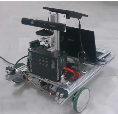
In this section, the robustness of AUKF to high sensor noise is validated in an indoor environment using a RGB-D based mobile robot. This robot explored an unknown and structured indoor environment, whilst it was building the map of the environment and localizing itself in this environment. The Microsoft XBOX Kinect was attached to the robot to obtain visual and depth information. The robot was controlled by two independent motors equipped by an incremental encoder. Combination of the differential driving output and gyro data were used for dead reckoning. The technical details about an approximated, discrete-time model of two-wheel driven mobile robot can be found in [31].

Kinect sensor camera has three lenses, an infrared transmitter for emitting a dotted light pattern, an Infrared CMOS camera for capturing reflected patterns, and a RGB camera for providing additional information on color and texture of the surface. The RGB camera supports a maximum resolution of 1280×960, while the depth sensors support 640×480 imaging. The view angles for the Kinect sensor cameras are 57 degrees horizontal and 43 degrees vertical. However, there is a practical ranging limit for extracting distance due to

depth sensing range for 0 to 4095 mm. Microsoft recommends extracting distance within the range of

1220 to 3810 mm for more accuracy and reliability. A mobile robot platform has been built in the Department of Mechanical Engineering of Yazd University, Yazd, Iran for indoor experiments (Fig. 8).

Figure 8. Experimental Robot Platform.

An Arduino board was used to collect data from sensors and to send them to a laptop for recording. The laptop was mounted on the robot to program the Arduino board, define the trajectory and record sensors data. When the robot navigated through the environment with a predefined trajectory, the estimated trajectory and the constructed map was recorded. The robot returned to the start point after detecting the environmental features using RGB-D sensor.

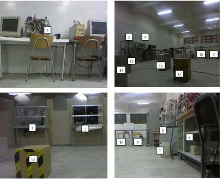
The Mechatronics Laboratory of Yazd University was chosen for obtaining the indoor dataset. This area spans a width of 7.3 meters by a length of 14 meters. A 2D location of objects and their dimension were collected from the environment to compare them with the estimated map obtained from the proposed algorithm. Unfortunately, the true trajectory was not available for

Table 2. MSE of UKF, EKF and AUKF estimations UKF EKF AUKF

κ = 3-nx without κ κ {0:0.5:4} κ {0:1:4} κ {0:1:10}

MSE 12.3720 19.8492 9.8808 10.0889 10.5084

Normalized time

44 the experiment like this. Several objects such as tables, chairs, boxes and experimental devices were placed in the environment. The true positions of objects were measured before running the algorithm. Several views of the environment along with a few objects are shown in Fig. 9.

Investigating the effectiveness of any SLAM algorithm requires detecting features. To extract the features from RGBD data, two processing steps were applied on the data. At the first step, an object detection method was applied on the RGBD data based on a combination of finding objects from depth image, and finding point correspondences between the reference and the target image. Then, the positions of these features were evaluated from the depth data. It must be noted that calibration of this sensor is necessary to measure the position of the features, accurately. A number of selected RGB and depth images along with

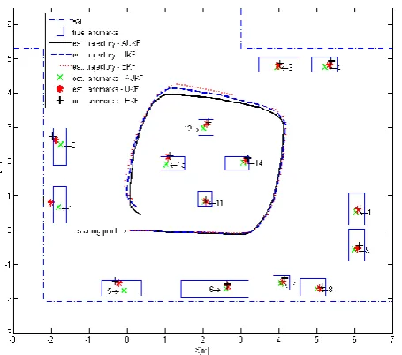
several features extracted during this experiment, are shown in Fig. 10. The constructed SLAM maps and trajectories of the robot using AUKF, UKF and EKF are also shown in Fig. 11. To demonstrate the applicability of AUKF-SLAM algorithm in real applications with higher number of search parameter, the values of κ are chosen by the grid method in the interval κ{0:0.5:10}. These experiments showed that AUKF-SLAM can be implemented in real-time applications. Comparison of the obtained results in Fig. 11 reveals that applying the proposed AUKF on the dataset improves the accuracy of SLAM, as compared to the standard UKF and EKF algorithms. The values of positions errors are plotted in Fig. 12. It can be seen that the proposed algorithm has the most accurate estimates as compared to the other methods.

45

Figure 10. RGB and depth images along with the extracted object. The red asterisks indicate the center position of extracted features.

Figure 11. Estimated map and the robot trajectories using AUKF, UKF and EKF algorithms by of the grid

method and the scaling parameter κ{0:0.5:10}.

46

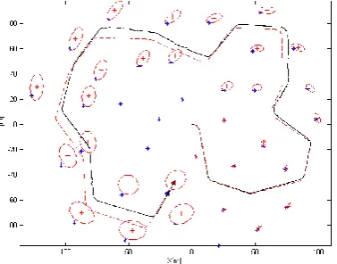
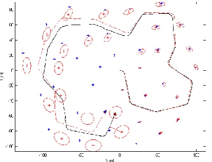
4.3. Victoria Park Dataset

Finally, the well-known Victoria Park dataset [25] is chosen to prove the applicability of the proposed method in large-scale environments. This dataset was recorded when a vehicle was driven around Victoria Park for about 25 minutes, covering a distance of over 4 km [25]. The vehicle was equipped with a GPS receiver in order to establish its trajectory. The control noises in the experiment are σV = 2 m/s, σγ = 6º, and the measurement

noises are σr = 1 m, σφ = 3º. Figure 13 presents the final

navigation map and vehicle trajectory estimated for a part of Victoria Park dataset by using the AUKF.

Figure 13. Estimated path (continuous line) and landmarks (plus sign with the uncertainty ellipse) using

AUKF for Victoria Park dataset.

Figure 14. Estimated path (continuous line) and landmarks (plus sign with the uncertainty ellipse) using AUKF for

Victoria Park dataset along with GPS data (points).

Since the true position of the vehicle was obtained with GPS, a true navigation map was available for

comparison purposes. It can be seen that the GPS sensor gave intermittent information due to limited satellite availability. Figure 14 shows estimated path and landmarks using AUKF algorithm for Victoria Park dataset along with GPS path that is represented by blue points.

5. Conclusions

In this work, an AUKF is applied on the SLAM problem in both simulated data and real application. The proposed adaptation of the scaling parameter is based on the maximum likelihood function at each time step. Through simulations, it is shown that the proposed approach decreases the estimation errors of the robot trajectory and the landmarks positions. MSE of the UKF and AUKF are compared by the impact of the chosen increment of the scaling parameter. It is shown that increasing the dimension of search space for the adaptation criteria leads to improving the accuracy of the estimation, although it adversely affects the required computational effort. Therefore, we should comprise between the wideness of the search space and the computational costs based on the required accuracy and available computational facilities. An RGBD dataset, obtained from a real setup, and Victoria Park dataset are used to demonstrate the applicability of the results for real navigations. The AUKF-SLAM algorithm described in this paper provides a more accurate method for estimating both the pose of the robot and the features in an unknown environment, as compared to the existing UKF and EKF methods.

6. Acknowledgements

This work is partially supported by Center of Excellence for Robust and Intelligent Systems (CERIS) of Yazd University.

7. References

[1] J. E. Guivant and E. M. Nebot, "Optimization of the simultaneous localization and map-building algorithm for real-time implementation," Robotics and Automation, IEEE Transactions on, vol. 17, pp. 242-257, 2001.

47

[3] M. Montemerlo, S. Thrun, D. Koller, and B. Wegbreit, "FastSLAM: A factored solution to the simultaneous localization and mapping problem," in AAAI/IAAI, 2002, pp. 593-598.

[4] V. Elvira, J. Míguez, and P. M. Djurić, "Adapting the number of particles in sequential monte carlo methods through an online scheme for convergence assessment,"

IEEE Transactions on Signal Processing, vol. 65, pp. 1781-1794, 2017.

[5] D. Simon, Optimal state estimation: Kalman, H infinity, and nonlinear approaches: John Wiley & Sons, 2006. [6] R. Martinez-Cantin and J. Castellanos, "Unscented SLAM

for large-scale outdoor environments," in Intelligent Robots and Systems, IEEE/RSJ International Conference

on, 2005, pp. 3427-3432.

[7] N. Sunderhauf, S. Lange, and P. Protzel, "Using the unscented kalman filter in mono-SLAM with inverse depth parametrization for autonomous airship control," in Safety, Security and Rescue Robotics, 2007. SSRR 2007. IEEE International Workshop on, 2007, pp. 1-6. [8] G. P. Huang, A. Mourikis, and S. Roumeliotis, "On the

complexity and consistency of UKF-based SLAM," in

Robotics and Automation, IEEE International Conference on, 2009, pp. 4401-4408.

[9] G. Shao, L. Wan, and X. D. Shen, "Hierarchical map building based UKF-SLAM approach for AUV," in

Applied Mechanics and Materials, 2013, pp. 793-797. [10] M. Wu and Y. Weng, "UKF-SLAM based gravity

gradient aided navigation," in Intelligent Robotics and Applications, ed: Springer, 2014, pp. 77-88.

[11] S. Maeyama, Y. Takahashi, and K. Watanabe, "A solution to SLAM problems by simultaneous estimation of kinematic parameters including sensor mounting offset with an augmented UKF," Advanced Robotics,

vol. 29, pp. 1137-1149, 2015.

[12] T. S. Ho, Y. C. Fai, and E. S. L. Ming, "Simultaneous localization and mapping survey based on filtering techniques," in Control Conference, 10th Asian, 2015, pp. 1-6.

[13] C. Cadena, L. Carlone, H. Carrillo, Y. Latif, D. Scaramuzza, J. Neira, et al., "Past, present, and future of simultaneous localization and mapping: toward the robust-perception age," IEEE Transactions on Robotics,

vol. 32, pp. 1309-1332, 2016.

[14] N. H. Khan and A. Adnan, "Ego-motion estimation concepts, algorithms and challenges: an overview,"

Multimedia Tools and Applications, pp. 1-23, 2016. [15] M. S. Bahraini, M. Bozorg, and A. B. Rad, "SLAM in

dynamic environments via ML-RANSAC,"

Mechatronics, vol. 49, pp. 105-118, 2018.

[16] M. Cugliari and F. Martinelli, "A FastSLAM algorithm based on the Unscented Filtering with adaptive selective resampling," in Field and Service Robotics, 2008, pp. 359-368.

[17] J. Qi, D. Song, C. Wu, J. Han, and T. Wang, "KF-based adaptive UKF algorithm and its application for rotorcraft UAV actuator failure estimation," Int J Adv Robotic Sy,

vol. 9, 2012.

[18] H. Wang, G. Fu, J. Li, Z. Yan, and X. Bian, "An adaptive UKF based SLAM method for unmanned underwater vehicle," Mathematical Problems in Engineering, vol. 2013, 2013.

[19] Z.-l. Wang, S. Qin, and Y.-m. Liang, "Adaptive UKF-SLAM Algorithm Based on Noise Scaling," Computer Engineering, vol. 10, p. 029, 2014.

[20] M. Wu and J. Yao, "Adaptive UKF-SLAM Based on Magnetic Gradient Inversion Method for Underwater Navigation," in Intelligent Robotics and Applications, ed: Springer, 2015, pp. 237-247.

[21] J. Dunik, M. Simandl, and O. Straka, "Unscented Kalman filter: aspects and adaptive setting of scaling parameter," Automatic Control, IEEE Transactions on,

vol. 57, pp. 2411-2416, 2012.

[22] L. A. Scardua and J. J. da Cruz, "Adaptively tuning the scaling parameter of the unscented kalman filter," in

Proceedings of the 11th Portuguese Conference on Automatic Control, 2015, pp. 429-438.

[23] O. Straka, J. Dunik, M. Simandl, and E. Blasch, "Comparison of adaptive and randomized unscented Kalman filter algorithms," in Information Fusion, 17th International Conference on, 2014, pp. 1-8.

[24] O. Straka, J. Dunik, and M. Simandl, "Unscented Kalman filter with advanced adaptation of scaling parameter," Automatica, vol. 50, pp. 2657-2664, 2014. [25] J. Guivant, J. Nieto, and E. Nebot, "Victoria park

48

[26] S. J. Julier and J. K. Uhlmann, "Unscented filtering and nonlinear estimation," Proceedings of the IEEE, vol. 92, pp. 401-422, 2004.

[27] S. Julier, J. Uhlmann, and H. F. Durrant-Whyte, "Technical Notes and Correspondence_," IEEE Transactions on automatic control, vol. 45, p. 477, 2000. [28] O. Straka, J. Dunik, and M. Simandl, "Scaling parameter in unscented transform: Analysis and specification," in

American Control Conference (ACC), 2012, 2012, pp. 5550-5555.

[29] T. Bailey, "Mobile robot localisation and mapping in extensive outdoor environments," Diss. The University of Sydney, 2002.

[30] T. Bailey, J. Nieto, J. Guivant, M. Stevens, and E. Nebot, "Consistency of the EKF-SLAM algorithm," in

Intelligent Robots and Systems, 2006 IEEE/RSJ International Conference on, 2006, pp. 3562-3568. [31] Y. Tu, Z. Huang, X. Zhang, W. Yu, Y. Xu, and B. Chen,

"The Mobile Robot SLAM Based on Depth and Visual Sensing in Structured Environment," in Robot Intelligence Technology and Applications 3, ed: Springer, 2015, pp. 343-357

Biography

Masoud S. Bahraini received his B.S. degree from Shahid Bahonar University of Kerman, Kerman, Iran (2009); and M.S. degree from Shiraz University, Shiraz, Iran (2012), both in Mechanical Engineering. He is currently a Ph.D. candidate in Mechanical Engineering Department of Yazd University, Yazd, Iran. He is also a research assistant at Autonomous and Intelligence Systems Laboratory (AISL), Simon Fraser University, Surrey, BC, Canada. His research interests include robot navigation, vibration analysis and control

Mohammad Bozorg received his B.S. and M.S. and Ph.D. degrees all in Mechanical Engineering from Chamran University of Ahwaz, Ahwaz, Iran, Sharif University of Technology, Tehran, Iran and Sydney University, Sydney, Australia in 1989, 1991 and 1997, respectively. In November 1997, he joined the Department of Mechanical Engineering, Yazd University, Yazd, Iran, where he is currently an associate professor. His current research interests include sensor fusion, navigation, robust control and mechatronics. He is a member of "Control Design" Technical Committee of International Federation of Automatic Control (IFAC) and a founding member of Robotic Society of Iran (RSI).