Volume 14 - Article 9 | Pages 157–178

in the population sciences published by the Max Planck Institute for Demographic Research Konrad-Zuse Str. 1, D-18057 Rostock·GERMANY www.demographic-research.org

DEMOGRAPHIC RESEARCH

VOLUME 14, ARTICLE 9, PAGES 157-178

PUBLISHED 07 MARCH 2006

http://www.demographic-research.org/Volumes/Vol14/9/ DOI: 10.4054/DemRes.2006.14.9

Research Article

A model for geographical variation

in health and total life expectancy

Peter Congdon

c

1 Introduction 158

2 The proportionality assumption (multiplicative model) 158

3 A model based on proportionality 160

4 Estimation 162

5 Modelling non-proportional age and area effects 166

6 Other models for age effects and spatially varying age effects 169

7 Implications for life table parameters 171

8 Conclusions 172

A model for geographical variation

in health and total life expectancy

Peter Congdon1

Abstract

This paper develops a joint approach to life and health expectancy based on 2001 UK Census data for limiting long term illness and general health status, and on registered death occurrences in 2001. The model takes account of the interdependence of different outcomes (e.g. ill health and mortality) as well as spatial correlation in their patterns. A particular focus is on the proportionality assumption or ’multiplicative model’ whereby separate age and area effects multiply to produce age-area mortality rates. Alternative non-proportional models are developed and shown to be more parsimonious as well as more appropriate to actual area-age interdependence. The application involves mortality and health status in the 33 London Boroughs.

1.

Introduction

Health expectancy is increasingly emphasised as an indicator for population health that takes account of both mortality and morbidity or disability. While morbidity and dis-ability data are often only obtainable from surveys, the recent UK 2001 Census includes questions on both limiting long term illness and general health status. Thus, in England and Wales63%of adults (aged16and over) said they had good health,26%reported they had fairly good health and11%said their health was not good. A variety of measures of health expectancy are available that may be based on limited function or self-perceived health status; these include disability free life expectancy and healthy life expectancy (Bebbington et al, 1993; Robine and Ritchie, 1991).

While both total life expectancy and health expectancy have improved in the UK, there are wide variations between geographic areas and socio-economic groups. Anal-yses of such contrasts, especially of spatial variations, have typically used standard life table calculations. These do not take account of features such as interdependence of dif-ferent outcomes (e.g. ill health and mortality), or of spatial correlation in their patterns, or of sampling variations in deaths or other outcomes. Where statistical modelling tech-niques are adopted, simplifying assumptions about the impacts of demographic variables and area are often made; for example, the proportionality assumption or ‘multiplicative model’ (Hoem, 1987) whereby separate age and area effects multiply to produce age-area mortality rates.

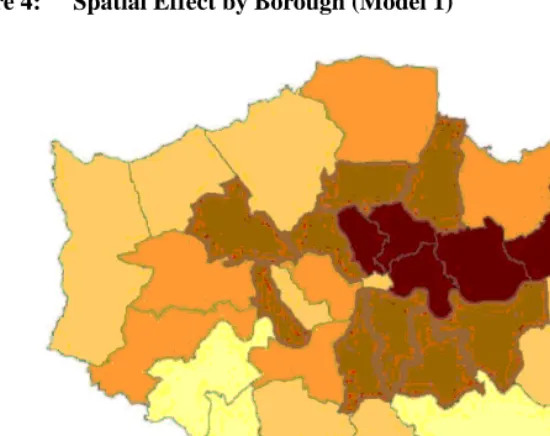
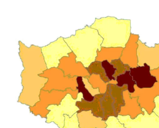
The present paper considers how evidence from mortality, limiting illness and self-rated health for sets of areas may be integself-rated in life tables for sets of contiguous areas. It includes consideration of the validity of the multiplicative model, and considers how interactions between age and area effects may be parsimoniously modelled. The appli-cation involves the33London Boroughs (Figure 1) and combines information from the two 2001 Census questions on disabling illness and self assessed health with recorded deaths in 2001 for the same areas. The result is a joint life table model for life and health expectancies by area.

2.

The proportionality assumption (multiplicative model)

Let populations in areaa(a= 1, . . . , A), and age bandx(x= 1, . . . , X)be denotedP_ax. Then deathsD_axby area and age band will be binomial

D_ax|µ_ax∼Bin(P_ax, µ_ax)

In line with many spatial epidemiology studies (e.g. Wakefield et al, 2000), the propor-tionality assumption is that

Figure 1: The London boroughs

whereρ_a are unknown relative risks for areaaandr_xare death rates at agex. For rare outcomes, the binomial distribution may be approximated by a Poisson distribution for theD_ax(e.g. Sun et al, 2000, p. 2108)

D_ax∼Poi(P_axµ_ax)

where µ_ax is often taken as proportional as in (1). A relevant model (e.g. with log link) forµ_axwould then takelog(ρ_a)andlog(r_x)as independent effects. Alternatively under the proportionality assumption one may collapse over the age groups to obtain a model where the area death totalsD_a = _xD_axare Poisson with meansE_aρ_a where

E_a =_xP_axr_xare expected deaths. If an internal demographic standardisation is used then_aD_a =_aE_aand so theρ_awill have average1, and posterior densities forρ_a concentrated on values over1(e.g. with95%credible interval all above1) then indicate excess relative risk in areaa.

assump-tion is that age effects are independent of area (e.g. McNab and Dean, 2001), though changes over time in the age profile of mortality may be included (Sun et al, 2000).

The present analysis uses age and area classifiers only and considers either total deaths (males and females combined) or deaths for one sex only. Extensions to include more classifiers (e.g. time) or to bivariate life table analysis (male and female life tables in one overall model) are, however, possible. Life and health expectancy may be jointly modelled for a set of areas using data on health status and long term illness as well as mortality data. An initial analysis using the proportionality assumption for these outcomes is contrasted in terms of fit and substantive implications with an analysis allowing for age-area interactions. The age-age-area interaction model draws on the principles in the Carter and Lee (1992) model for age-time interactions in mortality, and the related log-linear model of Goodman (1979). More heavily parameterised models that use random effects for each age-area interaction are also considered.

3.

A model based on proportionality

The relevant data are deathsD_axfor the year 2001, numbers of long term ill in areaa at agex,G_ax, and the numbersH_axj in areaaand agexin thej = 1, . . . ,3categories of the general health (good, fairly good, not good). There area = 1, . . . ,33areas and

x= 1, . . . ,19age bands (namely0−4,5−9, . . . ,85−89,over90).

Lets_adenote spatially correlated area effects,u_abe random errors without any spatial structure, andδ_x denote age effects. To reflect correlated outcomes one may include a common spatial effect across the responses, since it is plausible that a common structure between excess mortality and morbidity exists and that it follows a spatial structure. Then coefficientsθ_jmay be introduced to express the differential impact ofs_aon each outcome

j. Hence thes_acan be seen as a spatially correlated factor scores, andθ= (θ₁, θ₂, ..)as factor loadings, that account for correlations between the outcomes. Ifvar(s_a)is taken as a free parameter then for identifiability oneθcoefficient is assigned a set value (e.g.

θ₁= 1), while ifvar(s_a)is set, e.g.var(s_a) = 1, allθcoefficients may be free.

Several models are possible for age effects. Sun et al (2000) treat them as fixed ef-fects; McNab and Dean (2001) and Nandram et al (1999) use spline models; Ibrahim et al (2001) suggest random walks, while demographic applications (Anson, 1991) may use polynomials in age. Here the first two models use a random effects approach combin-ing a structured random walk prior with unstructured age effects. Thus withjdenoting mortality/morbidity responses(j= 1, ..K)

δ_jx=v_jx+w_jx

effects with w_jx ∼ N(0, ϕ_j). To reflect the correlation among the outcomes j it is assumed that rather than separate state space models for each of theK series of effects

v_jx, the processes are interlinked according to

v_jx =φ_jV_x

where theφ_jare loadings on a shared structured age effect

V_x∼N(V_x−1, ξ).

One possible model (model 1) for deaths and long term illness totals based on age-area proportionality is then

D_ax∼Po(P_axµ_ax)

log(µ_ax) =α₁+φ₁V_x+w_1x+θ₁s_a+u_1a (1a)

G_ax ∼Bin(P_ax, λ_ax)

logit(λ_ax) =α₂+φ₂V_x+w_2x+θ₂s_a+u_2a (1b)

whereα_jare intercepts. For numbersH_axkin the health status groups, a cumulative logit model involving

υ_axj =π_ax1+· · ·+π_axj=Pr(H_axk≤j), j= 1, J−1

(J = 3here) is often assumed. Other links allowing for asymmetric departures from the cumulative logit might also be considered such as the cumulative log-log link or links involving a transformation parameter (Zayeri et al, 2005; Agresti, 2002). A proportional cumulative logit model would require common age gradients and area effects acrossj. In the current application considerable gains in fit were made if age gradients and area effects were allowed to differ between levels of health status, leading to a non-proportional model (Peterson and Harrell, 1990). WhileJ−1non-parallel regression lines may cross when explanatory variables are continuous, this problem does not occur for explanatory variables that are categorical, as here (Gibbons and Hedeker, 2000). The cumulative logit model is then

logit(υ_ax1) =κ₁−(φ₃V_x+w_3x+θ₃s_a+u_3a) (1c)

logit(υ_ax2) =κ₂−(φ₄V_x+w_4x+θ₄s_a+u_4a) (1d)

The probabilitiesπ_axj of the health status distribution (H_ax1, H_ax2, H_ax3) in areaaand agexare obtained as

π_ax1=υ_ax1 π_ax2=υ_ax2−υ_ax1 π_ax3= 1−υ_ax2

The ICAR prior of Besag et al (1991) is used for the shared spatial effectss_a. Define theA×Acontiguity matrixCwith elementsc_ab=c_ba= 1if areasaandbare adjacent and zero otherwise, letL_a be the neighbourhood of areas adjacent to a (excluding area a itself) and letN_abe the number of areas in the neighbourhood. Then the Normal version of the ICAR prior (with varianceτ) assumes

f(s_a|s_[−a]) =

_N

a

2πτ

0.5

exp{−0.5Na

τ (sa−Sa)2}

wheres_[−a]denotes all{s₁, s₂, ..s_A}excepts_a, andS_ais the average ofs_bfor the areas

bin the localityL_aof areaa. Equivalently

s_a|s_[−a]∼N(

b

c_abs_b, τ /N_a)

To ensure identification thes_aare recentred at each iteration to have mean zero. Theu_ja are taken to be unstructured Normal random effects with mean zero.

Note that a close fit to the data may be attained by effectively modelling each ob-servation, namely adding random age-area effects{e_1ax, e_2ax, e_3ax, e_4ax} in (1a)-(1d). However, this approach is heavily parameterised, and leads to complex interpretation is-sues of model results in substantive terms. Instead the goal is relatively parsimonious and interpretable models that clearly improve fit as an alternative to introducing age-area interaction effects. This objective is pursued in subsequent model elaboration.

4.

Estimation

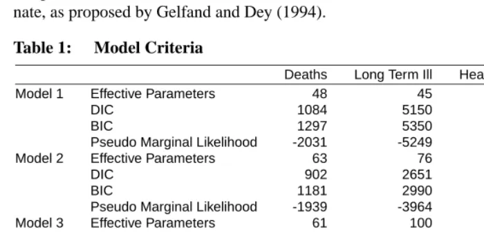
To assess model fit, one criterion used is the DIC of Spiegelhalter et al (2002), un-der which the number of effective parametersp_eis derived as the difference between the averaged sampled deviance Dev and the deviance atΦ, the posterior mean of the full pa-rameter setΦ. The DIC is then the average deviance plus the effective parameter total (see Table 1 for fit statistics for model 1 and subsequent models). Another is the pseudo marginal likelihood based on the Monte Carlo estimate of the conditional predictive ordi-nate, as proposed by Gelfand and Dey (1994).

Table 1: Model Criteria

Deaths Long Term Ill Health Status Total

Model 1 Effective Parameters 48 45 72 165

DIC 1084 5150 7950 14184

BIC 1297 5350 8319 14916

Pseudo Marginal Likelihood -2031 -5249 -9178 -16458

Model 2 Effective Parameters 63 76 154 293

DIC 902 2651 4611 8164

BIC 1181 2990 5404 9467

Pseudo Marginal Likelihood -1939 -3964 -7464 -13367

Model 3 Effective Parameters 61 100 194 355

DIC 904 2278 3987 7169

BIC 1175 2722 4983 8746

Pseudo Marginal Likelihood -1928 -3744 -7114 -12786

Model 4 Effective Parameters 159 467 905 1531

DIC 868 1154 2291 4313

BIC 1574 3228 6937 11112

Pseudo Marginal Likelihood -1920 -3126 -6181 -11227

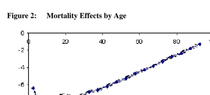
Figure 2: Mortality Effects by Age

5.

Modelling non-proportional age and area effects

To allow for non-proportional impacts means age effects and area effects will interact. As noted above, the most heavily parameterised models allowing this are random ef-fects models with termse_jaxspecific to area, age and outcome. These would usually be assumed spatially unstructured, though for a small number of age groupsxone might assumee_ja1, e_ja2, . . . ,etc to have distinct spatially correlated densities.

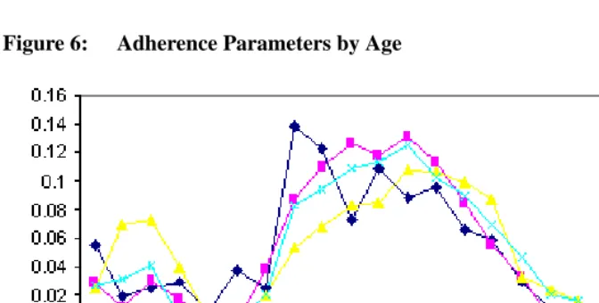
Alternatively for a relatively parsimonious model with substantive interpretability one may adapt the Carter-Lee model for forecasting mortality (Carter and Lee, 1992) to the present spatial application. The Carter-Lee model for mortality rates in age and timeµ_tx (without an area dimension) takes the form

log(µ_tx) =α₁+δ_x+β_xκ_t

with constraints on the multiplicative functionβ_xκ_tto ensure identifiability. Lee (2000) assumes theβ_x to be positive and sum to1over allx, and constrains the κ_tto sum to zero. Theβ_xparameters express variations between ages in the adherence to the overall mortality trend represented by theκ_t parameters. If theκ_twere declining as mortality fell then largerβ_xindicate for which age groups the rates are declining more rapidly.

In the present spatial mortality application one may incorporate this form of non-proportionality (leading to model 2). This involves first re-defining the mortality model as

D_ax∼Po(P_axµ_ax)

log(µ_ax) =α₁+δ_1x+β_1xγ_a+u_1a (2a)

where theβ_1xare assumed positive and sum to1and theγ_a are centred to sum to zero. The mixed random effects model for the age effectsδ_jx used in model (1) is retained in model 2. The remaining components of the model are redefined as

logit(λ_ax) =α₂+δ_2x+β_2xγ_a+u_2a (2b) logit(γ_ax1) =κ₁−(δ_3x+β_3xγ_a+u_3a) (2c) logit(γ_ax2) =κ₂−(δ_4x+β_4xγ_a+u_4a) (2d)

childhood and middle age bands, but low at old ages. Disability or poor health in middle age also tends to be elevated in deprived areas.

Extensions of the basic non-proportional model with generic form

log(µ_ax) =α+δ_x+u_a+β_xγ_a

may be envisaged. For example, it may be that there are discordant spatial effects or that the interaction between age and spatial effects is less clearly defined in some areas than others. The generic model reduces to the proportional model

log(µ_ax) =α+δ_x+u_a+γ_a

when all theβ_xare equal, so one might propose a two group discrete mixture whereby in one group theβ_xvary less than in another group. Thus

log(µ_ax) =α+δ_x+u_a+β_xGaγ_a

whereG_a ∈(1,2). One possible prior for theβ_xinvolves a multiple logit link, namely

β_x= exp(a_x)/

1 +X−1

x=1

exp(a_x)

x= 1, . . . , X−1

β_X = 1/

1 +X−1

x=1

exp(a_x)

wherea_xare random effects, e.g.a_x∼N(0, τ_a). So the discrete mixture would involve constrainingτ_ato be lower in one group than the other. Another possible model allowing for spatial outliers would mix over a normal ICAR spatial effectγ_1a and a heavy tailed (e.g. Laplace) spatial effectγ_2a. This can be done using continuous mixing using beta weightsh_a∼Beta(g₁, g₂)whereg₁andg₂are known (Lawson and Clark, 2002). So

log(µ_ax) =α+δ_x+u_a+β_x[h_aγ_1a+ (1−h_a)γ_2a].

Figure 6: Adherence Parameters by Age

6.

Other models for age effects and spatially varying age effects

Instead of assuming a random walk prior for the structured component in the age mixture model δ_jx = v_jx+w_jx, one might represent v_jx by a basis function (e.g. a polyno-mial spline or B spline), and then assume spatially varying coefficients applied to certain components in each function. This may be combined with predictor selection on other components of the function, leading to averaging over a number of different models. As noted by Smith and Kohn (1996) this implies a nonparametric regression model for age effects in which several predictor variables may be redundant. Here a cubic spline in age with terms{x, x2, x3,(x−t₁)3₊, . . . ,(x−t_M)3₊} is assumed in a third model. Define

B₁(x) = x, B₂(x) = x2_{, . . . , BM+3(x) = (x−tM)}3

+ then the smooth in age has the form

v_jx =M+3

k=1

g_jkη_jkB_k(x)

whereg_jkare binary selection indicators with Bernoulli(0.5) priors, andη_jkare coeffi-cients applied toB_k(x)only wheng_jk= 1. The linear coefficient in ageη_j1is taken as necessary by default so thatg_j1= 1(e.g. see Figures 2 and 3). All other terms are subject to predictor selection. TheMpotential knots are taken as the mid-points of each five year age band, excluding the first and last so there are seventeen potential knots (at ages7.5, 12.5, etc. to87.5). An unstructured random age termw_jxis retained to model remaining residual age impacts for outcomej.

and illness outcomes, so that linear coefficient in age for outcomejis area specific,η_j1a. There is evidence at a higher geographical scale, for example, that high and low mortality regimes in developed societies may differ in their age slopes (Gakidou et al, 2000). To additionally reflect the correlation between outcomes (death, long term limiting illness, etc) the area linear effect on age is modelled as

η_j1a =ω_ja+ψ_jξ_a

whereξ_a is a shared spatially correlated error,ω_jais an outcome specific unstructured error with meanη_j1andψ_jare outcome specific loadings. The remainder of the model is an in model 2.

Then model 3 for mortality is

log(µ_ax) =α₁+w_1x+ (ω_1a+ψ₁ξ_a)x+ [g₁₂η₁₂x2_+g

13η13x3+

g₁₄η₁₄(x−t₁)3

++· · ·+g1,M+3η1,M+3(x−tM)3+]+

β_1xγ_a+u_1a (3a)

The models for illness and health status are accordingly

logit(λ_ax) =α₂+w_2x+ (ω_2a+ψ₂ξ_a)x+ [g₂₂η₂₂x2_+g

23η23x3+

g₂₄η₂₄(x−t₁)3

++· · ·+g2,M+3η2,M+3(x−tM)3+]+

β_2xγ_a+u_2a (3b)

logit(γ_ax1) =κ₁−(w_3x+ [ω_3a+ψ₃ξ_a]x+{g₃₂η₃₂x2_+g

33η33x3+

g₃₄η₃₄(x−t₁)3

++· · ·+g3,M+3η3,M+3(x−tM)3+}+

β_3xγ_a+u_3a) (3c)

logit(γ_ax2) =κ₂−(w_4x+ [ω_4a+ψ₄ξ_a]x+{g₄₂η₄₂x2_+g

43η43x3+

g₄₄η₄₄(x−t₁)3

++· · ·+g4,M+3η4,M+3(x−tM)3+}+

β_4xγ_a+u_4a (3d)

As compared to model 2 this representation produces a further gain in fit at the ex-pense of a relatively small increase in the effective parameter total. The spatially varying linear age effectsη_j1a tend to be higher in deprived boroughs, but the correlation with deprivation is higher for health and illness outcomes than for mortality.

status analysis. For the mortality analysis this is only slight with Dev(Φ) = 782but for illness the same quantity is2078, while for health status it is3599. As mentioned above one generalisation of model 1 or subsequent models is to include unstructured age-area random effects (Dean et al, 2001). So let effectse_jaxreplace the unstructured are effects

u_jain model 2.

This leads to model 4

log(µ_ax) =α₁+δ_1x+β₁s_a+e_1ax (4a) logit(λ_ax) =α₂+δ_2x+β₂s_a+e_2ax (4b) logit(γ_ax1) =κ₁−(δ_3x+β₃s_a+e_3ax) (4c) logit(γ_ax2) =κ₂−(δ_4x+β₄s_a+e_4ax) (4d)

where thee_jaxare assumed to be unstructured with outcome specific variances

e_jax∼N(0, τ_ej).

While producing a clear reduction in the average deviance, this approach also has a cost in model complexity. The effective parameter total of around1500compares to the number of categories being modelled, namelyN_c= (19×33)+(19×33)+(2×19×33) = 2508.

Alternative measures of fit such as the BIC that penalise complexity more heavily than the DIC (or its classical equivalent the AIC) are available. There is evidence that the AIC tends to select complex models, i.e. is prone to overfitting (Geweke and Meese, 1981). An informal definition of the BIC that uses the effective parameter estimate for each of the three outcomes is contained in Table 1. This is based on the average deviance plus the product of the effective parameters by the log of the number of categoriesN_c being modelled:

BIC=Dev(Φ) +p_elog(N_c).

Although model 4 has a relatively low DIC and the highest pseudo marginal likeli-hood, its BIC exceeds those for the less complex models. Model 3 has the lowest BIC.

7.

Implications for life table parameters

a) life expectancy by area at agex,E_ax;

b) disability free life expectancyW_ax1 , namely years to be lived beyond agexbefore the onset of limiting long term illness;

c) healthy life expectancyW_ax2 , in terms of years to be lived in good health beyond agex

d) G1_ax, average years lived with disability, namely the gap betweenE_axandW_ax1; e) and average years lived in poor healthG2_ax, the gap betweenE_axandW_ax2 .

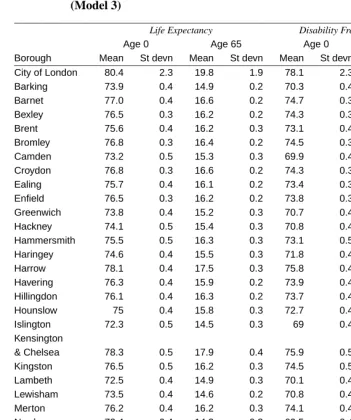
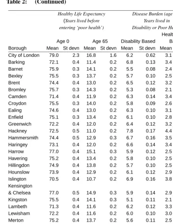
Table 2 shows posterior means and standard deviations by borough for total life ex-pectancy and the two forms of health exex-pectancy (at birth and age65) under model 3. Table 2 also contains a deprivation index devised by the UK Department of Environment, Transport and Regions. For example, the disability free life expectancy at birthW_a1₀varies from69to78.1and correlates−0.85with deprivation.

In terms of the disease burden at age65, Table 2 shows that years lived in poor health

G2

a,65after age65is typically around three years, or half of the years lived in disability

G1

a,65. Hence the worst category of the health status question is apparently identifying more severe morbidity than the long term illness (limiting disability) question. There is a0.95correlation between the disease burden measureG2_a,65and deprivation. ForG1_a,65 the correlation with deprivation is slightly lower, namely0.92.

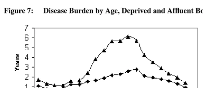
Of interest for health needs profiling is the disease burden at different ages and how this varies between geographic areas. As noted above the area gradients for illness on ageη_j1a are more highly correlated with area deprivation than those for mortality. This implies that the age profile of the disease burden would be discrepant between affluent and deprived boroughs, and Figure 7 contrasts the burden-age profile for the deprived inner city borough of Tower Hamlets with that in the affluent suburban area of Bromley. The clear excess in morbidity in the inner city borough, especially in middle ages, can be seen.

8.

Conclusion

This paper has sought to develop and investigate the fit of a set of models that depart from the often used proportionality assumption for mortality and morbidity data which are crossed by age and area. Instead relatively parsimonious models for age-area interactions in data on deaths and health in London have shown that the proportionality assumption is very much a simplification that does not match actuality for this city region.

Table 2: Life Table Parameters, Mortality and Health, London Boroughs (Model 3)

Life Expectancy Disability Free Life Expectancy

Age 0 Age 65 Age 0 Age 65

Borough Mean St devn Mean St devn Mean St devn Mean St devn

City of London 80.4 2.3 19.8 1.9 78.1 2.3 13.6 1.3

Barking 73.9 0.4 14.9 0.2 70.3 0.4 8.1 0.1

Barnet 77.0 0.4 16.6 0.2 74.7 0.3 11.1 0.2

Bexley 76.5 0.3 16.2 0.2 74.3 0.3 10.5 0.2

Brent 75.6 0.4 16.2 0.3 73.1 0.4 9.7 0.2

Bromley 76.8 0.3 16.4 0.2 74.5 0.3 11.2 0.2

Camden 73.2 0.5 15.3 0.3 69.9 0.4 8.9 0.2

Croydon 76.8 0.3 16.6 0.2 74.3 0.3 10.8 0.2

Ealing 75.7 0.4 16.1 0.2 73.4 0.3 9.7 0.2

Enfield 76.5 0.3 16.2 0.2 73.8 0.3 10.1 0.2

Greenwich 73.8 0.4 15.2 0.3 70.7 0.4 8.8 0.2

Hackney 74.1 0.5 15.4 0.3 70.8 0.4 7.6 0.2

Hammersmith 75.5 0.5 16.3 0.3 73.1 0.5 9.6 0.2

Haringey 74.6 0.4 15.5 0.3 71.8 0.4 8.9 0.2

Harrow 78.1 0.4 17.5 0.3 75.8 0.4 11.6 0.2

Havering 76.3 0.4 15.9 0.2 73.9 0.4 10.1 0.2

Hillingdon 76.1 0.4 16.3 0.2 73.7 0.4 10.6 0.2

Hounslow 75 0.4 15.8 0.3 72.7 0.4 9.7 0.2

Islington 72.3 0.5 14.5 0.3 69 0.4 7.6 0.2

Kensington

& Chelsea 78.3 0.5 17.9 0.4 75.9 0.5 12.0 0.3

Kingston 76.5 0.5 16.2 0.3 74.5 0.5 11.2 0.2

Lambeth 72.5 0.4 14.9 0.3 70.1 0.4 8.7 0.2

Lewisham 73.5 0.4 14.6 0.2 70.8 0.4 8.6 0.1

Merton 76.2 0.4 16.2 0.3 74.1 0.4 10.6 0.2

Newham 72.4 0.4 14.3 0.3 69.5 0.4 6.9 0.1

Redbridge 76.1 0.4 16.2 0.2 73.7 0.4 10.0 0.2

Richmond 77.4 0.4 16.8 0.3 75.8 0.4 11.9 0.2

Southwark 73.3 0.4 15.3 0.3 70.6 0.4 8.7 0.2

Sutton 76.1 0.4 15.8 0.3 73.7 0.4 10.5 0.2

Tower Hamlets 72.1 0.4 14.2 0.3 69.1 0.4 6.8 0.2

Waltham Forest 73.6 0.4 14.7 0.2 70.9 0.4 8.5 0.2

Wandsworth 74 0.4 14.7 0.2 71.9 0.4 9.2 0.2

Table 2: (Continued)

Healthy Life Expectancy Disease Burden (age 65), DETR

(Years lived before Years lived in Deprivation entering ‘poor health’) Disability or Poor Health Index

Health Status Age 0 Age 65 Disability Based Based Borough Mean St devn Mean St devn Mean St devn Mean St devn

City of London 79.0 2.3 16.8 1.6 6.2 0.62 3.1 0.34 -0.88

Barking 72.1 0.4 11.4 0.2 6.8 0.13 3.4 0.07 0.68

Barnet 75.9 0.3 14.1 0.2 5.5 0.08 2.4 0.05 -0.84

Bexley 75.5 0.3 13.7 0.2 5.7 0.10 2.5 0.05 -0.91

Brent 74.4 0.4 13.0 0.2 6.5 0.12 3.2 0.06 0.41

Bromley 75.7 0.3 14.3 0.2 5.3 0.08 2.1 0.05 -1.12

Camden 71.4 0.4 11.9 0.2 6.3 0.14 3.4 0.09 0.56

Croydon 75.5 0.3 14.0 0.2 5.8 0.09 2.6 0.05 -0.52

Ealing 74.6 0.4 13.0 0.2 6.3 0.10 3.1 0.06 -0.14

Enfield 75.1 0.3 13.4 0.2 6.1 0.10 2.8 0.05 -0.13

Greenwich 72.2 0.4 12.0 0.2 6.4 0.12 3.2 0.06 0.56

Hackney 72.5 0.5 11.0 0.2 7.8 0.17 4.4 0.11 2.02

Hammersmith 74.4 0.5 12.9 0.3 6.7 0.16 3.5 0.09 0.12

Haringey 73.1 0.4 12.0 0.2 6.6 0.14 3.4 0.08 0.92

Harrow 77.0 0.4 15.1 0.3 5.9 0.12 2.5 0.06 -0.89

Havering 75.2 0.4 13.4 0.2 5.8 0.10 2.5 0.05 -0.85

Hillingdon 74.9 0.4 13.8 0.2 5.7 0.10 2.5 0.05 -0.7

Hounslow 73.9 0.4 12.9 0.2 6.1 0.12 2.9 0.06 -0.22

Islington 70.5 0.4 10.7 0.2 6.9 0.16 3.8 0.10 1.21

Kensington

& Chelsea 77.0 0.5 14.9 0.3 5.9 0.14 2.9 0.08 -0.62

Kingston 75.5 0.4 14.1 0.3 5.1 0.11 2.1 0.06 -1.32

Lambeth 71.3 0.4 11.6 0.2 6.2 0.12 3.3 0.07 0.66

Lewisham 72.2 0.4 11.6 0.2 6.0 0.10 3.0 0.06 0.56

Merton 75.2 0.4 13.7 0.2 5.6 0.11 2.5 0.06 -0.74

Newham 70.9 0.4 10.2 0.2 7.4 0.15 4.0 0.09 2.02

Redbridge 75.0 0.4 13.4 0.2 6.3 0.11 2.9 0.06 -0.49

Richmond 76.6 0.4 14.8 0.3 4.9 0.11 2.0 0.05 -1.47

Southwark 72.0 0.4 11.8 0.2 6.6 0.13 3.5 0.08 1.21

Sutton 74.9 0.4 13.6 0.2 5.3 0.10 2.2 0.05 -1.01

Tower Hamlets 70.4 0.4 9.9 0.2 7.4 0.16 4.3 0.11 2.36

Waltham Forest 72.3 0.4 11.6 0.2 6.2 0.12 3.1 0.07 0.34

Wandsworth 73.1 0.4 12.0 0.2 5.6 0.11 2.7 0.06 -0.37

Figure 7: Disease Burden by Age, Deprived and Affluent Boroughs Compared

age groups accord with a single spatial health index γ_a. Similarly the basic linear age effect on log death rates or logit illness/health rates may vary over areas.

In a joint life table pooling over outcomes it is important to model the correlation be-tween outcomes. The correlation over outcomes in both age and area impacts is reflected in

a) the pooled random walk effectV_xinδ_jxin models 1 and 2 b) the shared spatial effectsθ_js_ain model 1

c) the adherence by ageβ_jxγ_ainteracting with shared spatial effects in model 2, and d) the common area effect multiplied by an outcome specific loading in the linear age

effects in model 3, namelyη_j1a=ω_ja+ψ_jξ_a.

Further stratifiers may be introduced into such a framework, for example deaths, ill-ness and health may be specific for gender or ethnicity as well as for age and area. A time dimension could be added also.

References

Agresti, A. (2002). Categorical data analysis. Wiley, 2nd Edition.

Anson, J. (1991). Model mortality schedules: a parametric evaluation. Population Studies, 45:137–153.

Bebbington, J. (1993). Regional and social variations in disability-free life expectancy in great britain. In: Robine J-M, Mathers C, Bone I, Romieu, I, eds. Calculation of health expectancies: harmonization, consensus achieved and future perspectives. London: John Libbey.

Besag, J., York, J., and Molli´e, A. (1991). Bayesian image restoration with two appli-cations in spatial statistics. Annals of the Institute of Statistics and Mathematics, 43:1–59.

Carter, L. and Lee, R. (1992). Modeling and forecasting us sex differentials in mortality. International Journal of Forecasting, 8:393–411.

Dean, C., Ugarte, M., and Militino, A. (2001). Detecting interaction between random region and fixed age effects in disease mapping. Biometrics, 57:197–202.

Eames, M., Ben-Shlomo, Y., and Marmot, M. (1993). Social deprivation and premature mortality: regional comparison across england. British Medical Journal, 307:1085– 6.

Gakidou, E., Murray, C., and Frenk, J. (2000). Defining and measuring health inequality: an approach based on the distribution of health expectancy. Bulletin of the World Health Organisation, 78:42–54.

Gelfand, A. and Dey, D. (1994). Bayesian model choice: asymptotics and exact calcula-tions. J. Royal Statist. Soc., 56(B):501–514.

Gelman, A., Carlin, J., Stern, H., and Rubin, D. (1995). Bayesian data analysis. London: Chapman and Hall.

Geweke, J. and Meese, R. (1981). Estimating regression models of finite but unknown order. International Economic Review, 22:55–70.

Goodman, L. (1979). Simple models for the analysis of association in cross-classifications having ordered categories. Journal of the American Statistical Association, 74:537– 551.

Hoem, J. (1987). Statistical analysis of a multiplicative model and its application to the standardization of vital rates: a review. International Statistical Review, 55:119– 152.

Ibrahim, J., Chen, M., and Sinha, D. (2001). Bayesian survival analysis. Springer Verlag: New York.

Lawson, A. and Clark, A. (2002). Spatial mixture relative risk models applied to disease mapping. Statistics in Medicine, 21:359–370.

Lee, R. (2000). The lee-carter method for forecasting mortality, with various extensions and applications. North American Actuarial Journal, 4:80–93.

MacNab, Y. and Dean, C. (2001). Autoregressive spatial smoothing and temporal spline smoothing for mapping rates. Biometrics, 57:949–56.

Murray, C. and Lopez, A. (1996). The global burden of disease. Harvard University Press.

Nandram, B., Sedrank, J., and Pickle, L. (1999). Bayesian analysis of mortality rates for us health service areas. Sankhya, 61(B):145–165.

Newbold, K., Eyles, J., Birch, S., and Spencer, A. (1998). Allocating resources in health care: alternative approaches to measuring needs in resource allocation formula in ontario. Health and Place, 4:79–89.

Noble, M., Penhale, B., Smith, G., Wright, G., Dibben, C., Owen, T., and Lloyd, M. (2000). Indices of deprivation 2000. Regeneration Research Summary Number 31, Department of Transport, Environment and the Regions.

Peterson, B. and Harrell, F. (1990). Partial proportional odds models for ordinal response variables. Applied Statistics, 39:205–217.

Robine, J.-M. and Ritchie, K. (1991). Healthy life expectancy : evaluation of a new global indicator for change in population health. British Medical Journal, 302:457–460.

Spiegelhalter, D., Best, N., Carlin, B., and van der Linde, A. (2001). Bayesian measures of model complexity and fit. J. Royal Statist. Soc, 64(B):583–639.

Sun, D., Tsutakawa, R., Kim, H., and He, Z. (2000). Spatio-temporal interaction with disease mapping. Statistics in Medicine, 19:2015–2035.

Wakefield, J., Best, N., and Waller, L. (2000). Bayesian approaches to disease mapping. In Elliott P, Wakefield J, Best N, Briggs D (eds) Spatial Epidemiology; Methods and applications. Oxford University Press, Oxford, pages 106–127.