CONTINUOUS TIME REGIME-SWITCHING MODEL APPLIED TO
FOREIGN EXCHANGE RATE
ST ´EPHANE GOUTTE1,∗, AND BENTENG ZOU2
1Universit´e Paris 8, LED , 2 rue de la Libert´e, 93526 Saint-Denis Cedex, France 2CREA, Universit´e du Luxembourg, 162A Avenue de la Faiencerie, L-1511 Luxembourg
Copyright c⃝2013 Goutte and Zou. This is an open access article distributed under the Creative Commons Attribution
License, which permits unrestricted use, distribution, and reproduction in any medium, provided the original work is
properly cited.
Abstract. The continuous time modified Cox-Ingersoll-Ross (1985) stochastic model is employed, com-bining with the Hamilton (1989) type Markov regime-switching framework, to study daily foreign ex-change rates where all parameter values depend on the value of a continuous time Markov chain. The generalized Expectation-Maximization algorithm is applied to a more general class of regime switching models and used to study some exchange rate data. We compare the obtained results with non regime switching models and notice that the regime switching outcomes match much better the reality than the others without Markov switching; and two regimes in most of the cases are better than more regimes.
Keywords: foreign exchange rate; regime switching model; expectation-maximization algorithm;
finan-cial crisis.
2010 AMS Subject Classification: 91G70, 60J05, 91G30
1. Introduction
∗Corresponding author
E-mail addresses: [email protected] (S. Goutte), [email protected] (B. Zou) Received August 08, 2013
1
Math. Finance Lett. 2013, 2013:8
The Markov Switching model defines two or more states or regimes, and hence, it can present the dynamic process of variables of concern vividly and provide researchers and policy makers with a clear clue of how these variables have evolved in the past and how they may change in the future.
Engle and Hamilton(1990) first study the exchange rate behavior using the non mean-reverting Markov switching model based on quarterly data in the exchange rate during the period of 1973-1988, and find that Markov switching model is a good approximation to the series. Engle (1994) extends this work and studies whether the Markov switching model is a useful tool for describing the behavior of 18 exchange rates and he concludes that the Markov switching model fits well in-sample for many exchange rates, but the Markov model does not generate superior forecasts to a random walk or for the forward rate. Engle and Hakkio (1996) examine the behavior of the European Monetary System exchange rates using the Markov switching model and find that the changes in exchange rate match the periodic extreme volatility. Marsh (2000) goes one step further and studies the daily exchange rates of three countries against the US dollar by applying the Markov switching model and concludes that the data are well estimated by Markov switching model though the out-of-sample forecasting is very poor due to parameter instability. And Bollen et al. (2000) examine the ability of the regime-switching model to capture the dynamics of foreign exchange rates and their test shows that a regime-switching model with independent shifts in mean and variance exhibits a closer fit and more accurate variance forecasts than a range of other models though the observed option prices do not fully reflect regime switching information.
Recently, Bergman and Hansson (2005) notice that the Markov switching model is good to describe the exchange rates of six industrialized countries against the US dollar. Cheung and Erlandsson(2005) test three dollar-based exchange rates by quarterly and monthly data, respectively, and notice that monthly data shows “...unambiguous evidence of the presence of Markov switching dynamics”. Their findings suggest that “data frequency, in addition to sample size, is crucial for determining the number of regimes”. More recently, Ismail and Isa (2007) employ the Markov switching model to capture regime shifts behavior in Malaysia ringgit exchange rates against four other countries between 1990 and 2005. They conclude that the Markov shifting model is found to successfully capture the timing of regime shifts in the four series.
Except for the above mentioned work, Lopez (1996) studies the exchange rate market in the long run (and short run) by specially taking into account the central bank regime shift and claims that the central bank activity does have long term effects on exchange rates (except for the short term impacts).
to different crises and/or policies. Exchange rate regime changes and their effects on some key macroe-conomic variables are studied by Caporale and Pittis (1995), who offer some insight into the effects of some regime changes on the real world.
In this present paper, we would rather see from a different direction than them. That is, we would like to see how the exchange rate would follow if the macroeconomic regime switches? To capture the stochastic nature of the foreign exchange rate, we modify the Cox, Ingersoll and Ross (1985) stochastic interest rate model to measure the exchange rate, particularly with a mean reverting part. Furthermore, we also calibrate the model based on real daily exchange rate data from Jan. 2000 until May 2012. To understand and catch the complete information of switching regimes, we present an extended and generalized Expectation-Maximization algorithm and followed by some comparison with respect to some other non-regime-switching models. By dosing so, we are convinced that stochastic exchange rates, under the regime-switching model, can sharply catch the regime-switching time and period. In addition, we also observe that two types of regimes– good and bad economic performance (or normal and crisis periods)– is better for most of the exchange rates studies than more regimes. And that confirms again the data frequency argument of Cheung and Erlandsson (2005). The very recent paper of Naszodi (2011) is close to our idea of switching regime effects on exchange rate. However, our regime-shifting is more general than Naszodi (2011) in which the switching is only about the exchange rate regime changes “from free floating to a completely fixed one,” such as “the adoption of the Euro”.
Nonetheless, in doing so, we employ time series filtering and smoothing technique to smooth out the noisy data. This technique promises that our results capture more precisely the trend of exchange rates than the standard Hamilton’s Markov switching model, which could be over-affected due to noise in the data, and, hence, misleading the regime-switching results.
To our knowledge, this is the first time that the combination of Cox-Ingersoll-Ross (hereafter, in short CIR) framework with the Markov regime switching model is employed to study foreign exchange rates, though a similar idea is used recently by Driffill and Kenc(2009) in studying bonds prices; however, there is no data smoothing process in their work. In this paper, with refined and modified filtering and smoothing algorithm, we show that the regime-switching Cox-Ingersoll-Ross model fits better foreign exchange rate data than, firstly, non regime-switching CIR and, secondly, other non regime-switching models.
For the above findings of maximum likelihood, we employ an extension of the well-known Expectation-Maximization (EM) algorithm, which was named and explained first by Dempster, Laird and Ru-bin(1977). Our setting is developed in Hamilton (1989a, b) and generalized in Choi (2009) or more recently in Janczura and Weron (2011). In short, this algorithm works in two steps: firstly, the Ex-pectation step (E-step) where all the probabilities of the model are calculated based on the current estimation of parameters; then, secondly, using these probabilities, the Maximization step (M-step) is done by maximizing the expected log-likelihood found in the E-step, and update estimated parameters will be used in the next E-step. Nonetheless, these are classical likelihood maximization steps but the likelihood function is weighted with the probabilities calculated in E-step. Indeed, we work in a regime-switching model. Hence, we will use a generalization of the (EM)-algorithm in order to apply to our general regime-switching model.
This paper is arranged as following: Section 2 presents the exchange rate Cox-Ingersoll-Ross model with regime switching. Section 3 documents real data, refined and modified filtering and smoothing algorithm. Then, Section 4 presents the main findings including simulation analysis and different types of comparison results. Section 5 studies some forecasting and Section 6 concludes.
1. The model
In this section, we first introduce the notion of continuous time Markov chain on finite space, then general continuous time regime switching model is presented. Finally, some examples of real word regime-switching are followed. LetT(>0) be a fixed maturity time and denote by (Ω,F:= (Ft)[0,T],P) an underlying probability space.
Definition 1.1. Let (Xt)t∈[0,T] be a continuous time Markov chain on finite space S :={1,2, . . . , K}.
Denote FX
t :={σ(Xs); 0≤s≤t}, the natural filtration generated by the continuous time Markov chain X. The generator matrix ofX is then denoted by ΠX and it is given by
(1.1) ΠXij ≥0 if i̸=j for all i, j∈ S and ΠXii =−∑ j̸=i
ΠXij otherwise.
Remark 1.1. The quantityΠX
ij represents the intensity of the jump from statei to statej.
We can now give the definition of global regime switching model.
Definition 1.2. For all t ∈ [0, T], Let Xt be a continuous time Markov chain on finite space S :=
stochastic process (rt) which is solution of the stochastic differential equation given by
(1.2) drt= (α(Xt)−β(Xt)rt)dt+σ(Xt) (rt)
δ(Xt)dW
t with r0=r∈R+
where α(Xt), β(Xt), σ(Xt) andδ(Xt)are functions of the Markov chain X. Hence, they are constants which take values in α(S),β(S),σ(S)andδ(S)
α(S) :={α(1), . . . , α(K)} ∈RK∗, β(S) :={β(1), . . . , β(K)}, σ(S) :={σ(1), . . . , σ(K)} ∈RK+ and δ(S) :={δ(1), . . . , δ(K)} ∈RK
For allj∈ {1, . . . , K}, we impose the condition2α(j)≥σ(j)2 to ensure the positivity of the process r.
Remark 1.2. – The above (RS-M)model is a continuous time regime switching diffusion with driftµ(rt, Xt) = (α(Xt)−β(Xt)rt)and volatilityσ(rt, Xt) =σ(Xt) (rt)
δ(Xt). For simplicity, we
will denote the valuesα(Xt),β(Xt),σ(Xt)andδ(Xt)byαt,βt,σt andδt.
– The drift factor,(αt−βtrt), ensures mean reversion of the process towards the long run value αt
βt, with speed of adjustment governed by the strictly positive parameterβt. From economic point
of view, if the value ofβtis large then the dynamic of the process r is almost near the value of
the mean, even if there is a spike at timet∈[0, T]. Then, for a small time periodϵ, the value ofrt+ϵ will be again close to the value of the mean.
– α(S)∈RK∗ means that all values of the parameter α in each state have to be strictly positive, since we have the condition2α(j)≥σ(j)2, for every j ∈ S. Moreover, σ is the volatility so it
has to be positive. Hence,σ(S)∈RK+.
Remark 1.3. – It is obvious that in this model there are two sources of randomness: the Brownian motionW appearing in the dynamic ofrand the Markov chainX. Hence, there is a randomness
dues to the information market which is the initial continuous filtration F generated by the
Brownian motionW; and another randomness dues to the Markov chain X, FX. We assume
thatW andX are mutually independent.
– This independence implies that the Markov chain is an exogenous factor of the market infor-mation. Thus, it can be seen as an exogenous factor such as an economic impact factor. An
economic interpretation of this is that the Markov chain can represent a credit rating of a firm
A. Indeed, assume that(RS-M) models the spread of a firm A then the Markov chain can be
the credit rating of this firm given by an exogenous rating company as “Standard and Poors”.
Then it is natural to think that the dynamic of the spread of the firmA depends on the value of
Hence, model (RS-M)(1.2) is a mean reverting model with local volatility. Moreover, this model is construct to encompass most of the financial models stated in the literature. Indeed, we obtain :
•Regime switching Cox Ingersoll Ross (RS-CIR).
Takingδ(Xt)≡ 12, we obtain a standard Cox-Ingersoll-Ross (CIR) model with regime switching param-eters:
(1.3) drt= (α(Xt)−β(Xt)rt)dt+σ(Xt)√rtdWt.
•Regime switching Vasicek (RS-V).
Takingδ(Xt)≡0, it yields a Vasicek model with regime switching parameters:
(1.4) drt= (α(Xt)−β(Xt)rt)dt+σ(Xt)dWt.
•Regime switching mean reverting Geometric Brownian motion (RS-R-GM).
Taking δ(Xt) ≡ 1, we have a geometric Brownian motion with mean reverting and regime switching parameters:
(1.5) drt= (α(Xt)−β(Xt)rt)dt+σ(Xt)rtdWt.
•Regime switching Constant of elasticity Variance (RS-CEV)
Takingα(Xt)≡0, it follows a constant of elasticity variance (CEV) with regime switching parameters:
(1.6) drt=−β(Xt)rtdt+σ(Xt) (rt)δ(Xt)dWt.
In Europe, Ferrara (2008) employs Markov-switching model to construct probabilistic indicators and serves as useful tools for providing original qualitative information for economic analysis, especially “ to monitor on a monthly basis turning points in the business cycle in French industry and those in the acceleration cycles in the French economy as a whole” and “Indicators of this nature are currently being developed for the euro area as a whole”. Billio and Casarin’s (2010) recent working paper study the Euro area by considering monthly observation from January 1970 until May 2009 of the industrial production index. They find that their new class of Markov switching latent factor model (with stochastic transition probability) “implies a better description of the dynamics of the Euro-zone business cycle”.
Basing on the above facts that Markov switching models capture the economic cycles and regime switching, therefore, we would like to see how the exchange rates would behave, do the exchange rates follow the economic regime switching and how large (or small) are the effects?
In order to answer these questions, in the following sections, we first introduce some real data followed by some calibration, estimation, comparison with some other models, and some forecasting for exchange rates.
2. Data and Estimations Methods
In this section, we first state real foreign exchange rate data for different currencies. In order to study and get as much information as possible, we then present the Estimation Method: the extended and generalized Expectation-Maximization algorithm.
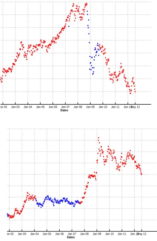
2.1. Data. Our samples of exchange rate include Euros VS Dollars, Yuan VS Dollars, Euro VS Yen, Euro VS Livre (GB) and Euro VS Yuan. Figure 1, 2 and 3 show the historical value of the corresponding daily foreign exchange rates over the period of January 1st, 2000 until May 28, 2012, except for the foreign exchange rate Yuan VS Dollars which begins in January 2006 since before it is a fixed constant.
Jan 02 Jan 03 Jan 04 Jan 05 Jan 06 Jan 07 Jan 08 Jan 09 Jan 10 Jan 11 Jan 12 May 12
Dates
Jan 06 Jan 07 Jan 08 Jan 09 Jan 10 Jan 11 Jan 12 6.2
6.4 6.6 6.8 7 7.2 7.4 7.6 7.8 8 8.2
Dates
Figure 1.
On left: Price of 1 Euro in Dollars between Jan. 2000 and May
2012. On right: Price of 1 Yuan in Dollars between Jan. 2006 and May 2012.
We begin by giving in Table 1 some general descriptive statistics for all foreign exchange rate data.
Datas Minimum Maximum Mean Std. Dev. Skewness Kurtosis
Euro/Dollars 0.8324 1.5849 1.2190 0.1965 -0.0033 0.0032
Yuan/Dollars 6.3809 8.0702 7.1376 0.5164 0.0771 0.1298
Euro/Yen 90.5300 168.77 127.9484 19.2980 2222.8422 312563.5673
Euro/Livre 0.5794 0.9610 0.72803 0.0994 0.0005 0.0002
Euro/Yuan 6.8839 11.1920 9.2032 1.1277 -0.4633 3.1990
Table 1.
Summary Statistics
It is easy to see that this historical data of exchange rates have significant different economic fluctu-ation during this time interval. To study the above presented data, we rely on an estimfluctu-ation method: Expectation-Maximization algorithm.
Jan 01 Jan 02 Jan 03 Jan 04 Jan 05 Jan 06 Jan 07 Jan 08 Jan 09 Jan 10 Jan 11 Jan 12May 12 Dates
Jan 01 Jan 02 Jan 03 Jan 04 Jan 05 Jan 06 Jan 07 Jan 08 Jan 09 Jan 10 Jan 11 Jan 12May 12 Dates
Figure 2.
On left: Price of 1 Euro in Livre (GB) between Jan. 2006 and May
2012. On right: Price of 1 Euro in Yen (Jap.) between Jan. 2006 and May 2012.
Jan 00 Jan 01 Jan 02 Jan 03 Jan 04 Jan 05 Jan 06 Jan 07 Jan 08 Jan 09 Jan 10 Jan 11 Jan 12May 12 Dates
Figure 3.
Price of 1 Euro in Yuan between Jan. 2006 and May 2012.
b) and studied recently by Choi (2009) and Janczura and Weron (2011). We applied this estimation method to our general regime switching model (1.2).
Suppose that the size of historical data isM+ 1. Let Γ denote the corresponding increasing sequence of time where this data value are taken:
Then, the discretized approximation model of (1.2) is given by
(2.7) rtk−rtk−1 =
(
αtk−βtkrtk−1
)
∆t+σtk(rtk−1)
δtk∆W
tk, for all k∈ {1, . . . , M}.
Here, the time step ∆t is equal to one since we have uniform equidistant time data values. Then, ∆Wtk ∼
√
∆tϵtk=ϵtk whereϵtk∼ N(0,1). Hence, it yields
rtk−rtk−1 =
(
αtk−βtkrtk−1
)
+σtk(rtk−1)
δtkϵ tk, rtk = αtk+ (1−βtk)rtk−1+σtk(rtk−1)
δtkϵ tk. (2.8)
We will denote in the sequel byFtrk the vector of historical value of the process r until timetk ∈Γ. Thus, Fr
tk is the vector of the k+ 1 last value of the discretized model defined in (2.8) and therefore,
Fr
tk = (rt0, rt1, . . . , rtk).
To estimate the optimal set of parameters ˆΘ :=
(
ˆ
αi,βˆi,σˆ2i,δˆi,Πˆ
)
, fori∈ S, we use the EM-algorithm where the set of parameter Θ is estimated by an iterative two-step procedure. First, the Expectation procedure or E-step: We evaluate the smoothed and filtered probability. In fact the filtered probability is given by the probability such that the Markov chain X is in regime i ∈ S at time t with respect to
Fr
t. And the smoothed probability is given by the probability such that the Markov chain X is in regime i ∈ S at time t with respect to all the historical data Fr
T. Second, the Maximization step, or M-step: We estimate all the parameters of the vector Θ using maximum likelihood estimation and the probability obtained in the E-step. More precisely, the process is giving as follow:
Proposition 2.1. The estimation method is given by the following procedure.
(1) Starting with an initial vector set Θ(0) := (α(0)
i , β
(0)
i , σ
2
i
(0)
, δi(0),Π(0)), for all i ∈ S. Fixed N ∈N, the maximum number of iteration we authorize for this method (for the step 2 and 3 of
EM-algorithm). And fixed a positive constantεas a convergence constant for the estimated log
likelihood function.
(2) Assume that we are at then+ 1≤N steps, calculation in the previous iteration of the algorithm yields vector setΘ(n):=
(
α(in), βi(n), σi2(n), δi(n),Π(n)
)
.
E-Step :: Filtered probability:: For all i ∈ S and k = {1,2, . . . , M}, evaluate the quantity
P
(
Xtk =i|F r tk; Θ
(n)) =
P
(
Xtk, rtk|F r tk−1; Θ
(n)) f
(
rtk|F r tk−1; Θ
(n))
= P
(
Xtk=i|F r tk−1; Θ
(n))f(r
tk|Xtk=i;F r tk−1; Θ
(n))
∑
j∈SP
(
Xtk=j|F r tk−1; Θ
(n)
)
f
(
rtk|Xtk =j;F r tk−1; Θ
(n)
)
with
P
(
Xtk=i|F r tk−1; Θ
(n)) = ∑
j∈S P
(
Xtk =i, Xtk−1 =j|F
r tk−1; Θ
(n))
= ∑
j∈S P
(
Xtk =i, Xtk−1 =j|Θ
(n))P(X
tk−1 =j|F
r tk−1; Θ
(n))
= ∑
j∈S Π(jin)P
(
Xtk−1 =j|F
r tk−1; Θ
(n)) (2.10)
where f
(
rtk|Xtk =i;F r tk−1; Θ
(n)) is the density of the process r at time t
k
condi-tional that the process is in regime i∈ S. Observed by (2.8), that given Fr tk−1, the process rtk has a conditional Gaussian distribution with mean
α(in)+
(
1−β(in)
)
rtk−1
and standard deviation σi(n)(rtk−1)
ˆ
δi(n), whose density function is given by
f
(
rtk|Xtk=i;F r tk−1; Θ
(n))= 1 √
2πσi(n)|rtk−1|
ˆ
δi(n) exp
− (
rtk−(1−β (n)
i )rtk−1−α
(n)
i
)2
2(σi(n))2|rtk−1|
2ˆδi(n)
. (2.11)
Smoothed probability:: For alli∈ S andk={M−1, M −2, . . . ,1},
P
(
Xtk=i|F r tM; Θ
(n))=∑
j∈S
(
P(Xtk =i|F r tk; Θ
(n))P(X
tk+1 =j|F
r tM; Θ
(n))Π(n)
ij P(Xtk+1 =j|F
r tk; Θ
(n))
)
. (2.12)
M-Step :: The maximum likelihood estimates Θ(n+1) for all model parameters is given, for all i∈ S, by
α(in+1) =
∑M k=2
[
P(Xtk=i|F r tM; Θ
(n))|r
tk−1|−
2δi(n)(r
tk−(1−β (n+1)
i )rtk−1
)]
∑M k=2
[
P(Xtk=i|F r tM; Θ
(n))|r
tk−1|−
2δi(n)] ,
βi(n+1) =
∑M k=2
[
P(Xtk=i|F r tM; Θ
(n))|r
tk−1|−
2δi(n)r tk−1B1
]
∑M k=2
[
P(Xtk=i|F r tM; Θ
(n))|r
tk−1|−
2δi(n)r tk−1B2
],
σi2(n+1) =
∑M k=2
[
P(Xtk=i|F r tM; Θ
(n))|r
tk−1|−
2δi(n)(r tk−α
(n+1)
i −(1−β
(n+1)
i )rtk−1
)2]
∑M k=2
[
P(Xtk =i|F r tM; Θ
(n))] ,
where
B1 = rtk−rtk−1−
∑M k=2
[
P(Xtk=i|F r tM; Θ
(n))|r
tk−1|−
2δi(n)(r
tk−rtk−1
)]
∑M k=2
[
P(Xtk =i|F r tM; Θ
(n))|r
tk−1|−
2δ(in)] ,
B2 =
∑M k=2
[
P(Xtk =i|F r tM; Θ
(n))|r
tk−1|−
2δ(in)r tk−1
]
∑M k=2
[
P(Xtk=i|F r tM; Θ
(n))|r
tk−1|−
The fourth parameterδi(n+1)is obtained by a numerical maximization of the likelihood func-tion. Finally, the transition probabilities are estimated according to the following formula
Π(ijn+1) =
∑M k=2
[
P(Xtk=j|F r tM; Θ
(n))Π
(n)
ij P (
Xtk−1=i|Ftkr
−1;Θ (n))
P (
Xtk=j|Fr tk−1;Θ
(n))
]
∑M k=2
[
P(Xtk−1 =i|F
r tM; Θ
(n))] .
(2.13)
(3) Denote by Θ(n+1) :=
(
α(in+1), βi(n+1), σ2i(n+1), δ(in+1),Π(n+1)
)
, the new parameters of the
algo-rithm and use it in step 2 until the convergence of the EM-algoalgo-rithm. In fact, we stop the
procedure if one of the following conditions are verified:
(a) We have done N times the procedure.
(b) The difference between the log likelihood at step n+ 1≤N denoted by logL(n+ 1) and at stepn, satisfied the relation
(2.14) logL(n+ 1)−logL(n)< ε.
Remark 2.4. (1) Proof of obtaining estimators α(in+1), βi(n+1) and σ2i(n+1) are demonstrated in Lemma 3.1 of Janczura and Weron (2011). Formula to obtain allΠ(ijn+1) are deduced from Kim (1994).
(2) Since the log likelihood function is increasing in each iteration of the procedure, we don’t need to take absolute value of the left hand side of inequality (2.14).
(3) In our case (i.e. regime switching), the standard log-likelihood function without regime switching
∑M k=1log
(
f
(
rtk|F r tk−1; Θ
(n))) has to be weighted with the corresponding smoothed inference.
Each observationrtk belongs to theith state with probabilityP
(
Xtk=i|F r tM; Θ
(n)). Hence, the
regime switching log-likelihood function is:
(2.15) L(Θ) =
M ∑ k=1 log ( f (
rtk|Xtk=i;F r tk−1; Θ
(n)))P(X
tk =i|F r tM; Θ
(n)).
(4) The standard error of each estimator is obtained by taking the square root of the(i, i)−th entry of the inverse of−H( ˆΘ) whereH( ˆΘ) is the Hessian matrix defined by
H( ˆΘ)i,j=
(
∂2L( ˆΘ) ∂Θi∂Θj
)
, i, j∈ S.
3. Main Findings and Models Comparison
Starting from a model with two regimes S = {1,2}, which represent two states of the economy: good and bad economic performance or a ”normal” and crisis economy. We would like to discover:
ii.: Regime switching against non regime switching models, does the regime switching model offers better results?
Based on general model (1.2), we have 5 regime switching models: the more general model (RS-M) given by (1.2), the models (RS-CIR), (RS-V), (RS-R-G(RS-M) and (RS-CEV). We will estimate the parameters of each model on each foreign exchange rate data. To run the estimation procedure, we need to take an initial parameters Θ(0). For this, we take an initial regime distribution equals to(12,12). That is, beginning with the same probability in each regime, we take an initial transition matrix Π(0) of the Markov chainX, such that, Π(0)11 = Π(0)22 = 12. And finally, initial parameters values(α(0), β(0), σ(0), δ(0)) are given by the results of a global maximum likelihood estimation on the corresponding models without regime shift.
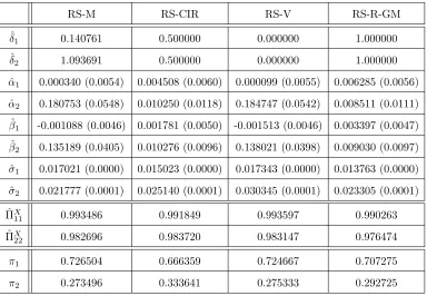
3.1. Parameters estimation. The Tables (2), (3), (4), (5) and (6) present values of the parameters estimation for each models.
RS-M RS-CIR RS-V RS-R-GM
ˆ
δ1 0.140761 0.500000 0.000000 1.000000
ˆ
δ2 1.093691 0.500000 0.000000 1.000000
ˆ
α1 0.000340 (0.0054) 0.004508 (0.0060) 0.000099 (0.0055) 0.006285 (0.0056) ˆ
α2 0.180753 (0.0548) 0.010250 (0.0118) 0.184747 (0.0542) 0.008511 (0.0111) ˆ
β1 -0.001088 (0.0046) 0.001781 (0.0050) -0.001513 (0.0046) 0.003397 (0.0047) ˆ
β2 0.135189 (0.0405) 0.010276 (0.0096) 0.138021 (0.0398) 0.009030 (0.0097) ˆ
σ1 0.017021 (0.0000) 0.015023 (0.0000) 0.017343 (0.0000) 0.013763 (0.0000) ˆ
σ2 0.021777 (0.0001) 0.025140 (0.0001) 0.030345 (0.0001) 0.023305 (0.0001) ˆ
ΠX
11 0.993486 0.991849 0.993597 0.990263
ˆ ΠX
22 0.982696 0.983720 0.983147 0.976474
π1 0.726504 0.666359 0.724667 0.707275
π2 0.273496 0.333641 0.275333 0.292725
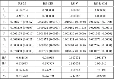
RS-M RS-CIR RS-V RS-R-GM ˆ
δ1 8.688204 0.500000 0.000000 1.000000
ˆ
δ2 -1.957911 0.500000 0.000000 1.000000
ˆ
α1 0.021557 (0.0067) 0.002560 (0.0177) 0.019259 (0.0060) 0.005650 (0.0182) ˆ
α2 0.005200 (0.0195) 0.019622 (0.0061) 0.000162 (0.0173) 0.020305 (0.0061) ˆ
β1 0.003125 (0.0010) 0.001503 (0.0025) 0.002820 (0.0009) 0.001943 (0.0026) ˆ
β2 0.001989 (0.0027) 0.002873 (0.0009) 0.001121 (0.0024) 0.002973 (0.0009) ˆ
σ1 0.000000 (0.0000) 0.006980 (0.0000) 0.003307 (0.0000) 0.002652 (0.0000) ˆ
σ2 0.871350 (0.0803) 0.001249 (0.0000) 0.018447 (0.0000) 0.000476 (0.0000) ˆ
ΠX11 0.881806 0.984915 0.957572 0.983178
ˆ ΠX
22 0.933623 0.956565 0.985652 0.954240
π1 0.359628 0.742231 0.252713 0.731195
π2 0.640372 0.257769 0.747287 0.268805
Table 3.
Maximum Likelihood estimation results for the Dollars-Yuan data
with standard errors.
RS-M RS-CIR RS-V RS-R-GM
ˆ
δ1 1.797463 0.500000 0.000000 1.000000
ˆ
δ2 -0.083423 0.500000 0.000000 1.000000
ˆ
α1 14.918395 (4.6358) 7.525180 (3.0508) 17.774657 (5.9303) 6.889107 (3.0148) ˆ
α2 -0.363333 (0.7003) 0.004430 (0.7695) 0.199365 (0.6992) 0.088266 (0.7828) ˆ
β1 0.122275 (0.0390) 0.068257 (0.0266) 0.143222 (0.0455) 0.062993 (0.0271) ˆ
β2 -0.003321 (0.0054) -0.000544 (0.0060) -0.002095 (0.0054) 0.000099 (0.0062) ˆ
σ1 0.000813 (0.0000) 0.397770 (0.0254) 5.199643 (5.8142) 0.035694 (0.0002) ˆ
σ2 3.143649 (0.6962) 0.183135 (0.0024) 2.129099 (0.3167) 0.016173 (0.0000) ˆ
ΠX
11 0.890571 0.966836 0.899831 0.970122
ˆ
ΠX22 0.988872 0.995772 0.991836 0.996123
π1 0.092303 0.113062 0.075357 0.114846
π2 0.907697 0.886938 0.924643 0.885154
RS-M RS-CIR RS-V RS-R-GM ˆ
δ1 -4.137988 0.500000 0.000000 1.000000
ˆ
δ2 3.049220 0.500000 0.000000 1.000000
ˆ
α1 0.018711 (0.0066) 0.008197 (0.0045) 0.008158 (0.0046) 0.006397 (0.0032) ˆ
α2 0.004255 (0.0043) 0.004782 (0.0074) 0.007253 (0.0090) 0.009330 (0.0137) ˆ
β1 0.028651 (0.0098) 0.011400 (0.0066) 0.011340 (0.0067) 0.008588 (0.0045) ˆ
β2 0.004260 (0.0061) 0.005297 (0.0094) 0.008402 (0.0110) -0.016901 (0.0202) ˆ
σ1 0.001188 (0.0000) 0.008090 (0.0000) 0.006728 (0.0000) 0.010927 (0.0000) ˆ
σ2 0.022192 (0.0000) 0.016107 (0.0000) 0.014717 (0.0000) 0.023550 (0.0001) ˆ
ΠX11 0.986823 0.996013 0.996129 0.996683
ˆ ΠX
22 0.993432 0.985484 0.985726 0.953937
π1 0.332644 0.784503 0.786676 0.932828
π2 0.667356 0.215497 0.213324 0.067172
Table 5.
Maximum Likelihood estimation results for the Euro-Livres data with
standard errors.
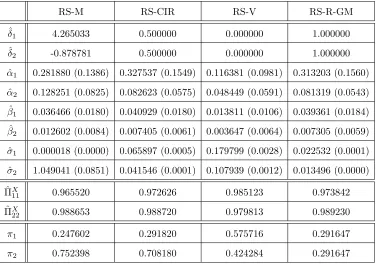
RS-M RS-CIR RS-V RS-R-GM
ˆ
δ1 4.265033 0.500000 0.000000 1.000000
ˆ
δ2 -0.878781 0.500000 0.000000 1.000000
ˆ
α1 0.281880 (0.1386) 0.327537 (0.1549) 0.116381 (0.0981) 0.313203 (0.1560) ˆ
α2 0.128251 (0.0825) 0.082623 (0.0575) 0.048449 (0.0591) 0.081319 (0.0543) ˆ
β1 0.036466 (0.0180) 0.040929 (0.0180) 0.013811 (0.0106) 0.039361 (0.0184) ˆ
β2 0.012602 (0.0084) 0.007405 (0.0061) 0.003647 (0.0064) 0.007305 (0.0059) ˆ
σ1 0.000018 (0.0000) 0.065897 (0.0005) 0.179799 (0.0028) 0.022532 (0.0001) ˆ
σ2 1.049041 (0.0851) 0.041546 (0.0001) 0.107939 (0.0012) 0.013496 (0.0000) ˆ
ΠX
11 0.965520 0.972626 0.985123 0.973842
ˆ
ΠX22 0.988653 0.988720 0.979813 0.989230
π1 0.247602 0.291820 0.575716 0.291647
π2 0.752398 0.708180 0.424284 0.291647
Where the quantitiesπ1 andπ2 represent the stationary distribution of the Markov chain given by
(π1, π2) =
(
1−ΠˆX
22 2−ΠˆX
11−ΠˆX22
, 1−Πˆ X
11 2−ΠˆX
11−ΠˆX22
)
.
Furthermore, it is clear that the presence of mean reverting effect (i.e. the parameter ˆβi) in each data can’t be rejected.
For each data, taking the model which obtain the higher log likelihood value (see Table (13)), we can plot Figures 10, 11 and 12 which give the evolution of the values of parameters in each regime during all the estimation procedure. In all the figures in this subsection, the regime 1 will be in color blue and regime 2 in color red. It is obvious that, in all the cases, convergence of the EM-Algorithm happens in less than 40 steps.
Figures 13, 14 and 15 give the smoothed and the filtered probabilities basing on real data. Usual-ly, “smoothed probabilities allow for the most information ex-post analysis of the data, while filtered probabilities are useful for forecasting” as stated by Calvet and Fisher (2008).
3.2. Value of the Regime duration time. Basing on and using the above estimations and classifi-cations, we can reproduce the exchange rates, whose origin real data are presented at the beginning of last section. Figures 4, 5 and 6 give trajectories of foreign exchange rate with respect to the value of the current regime. Again, we take the model which obtain the higher log likelihood value (see Table (13)).
The left graph in Figure 4 indicates clearly two significantly different time periods. The first one, in blue, corresponds to an increasing time period where the value of the change is better for Euro zone. This can be seen from the value of estimating parameters. Indeed, in this regime the speed of adjustment parameter ˆβ is close to zero ( ˆβ1= 0.001294) which means that the Euro-dollar exchange rate dynamic has a mean reversion close to zero. The second one, in red, corresponds to a more volatile time period where the volatility in this regime equals 0.025852 against 0.014986 as in regime 1. This shows an increasing of the volatility which equals to 72.51%. Hence, all the crisis periods fall into this regime which are the periods (1) between January 2000 and March 2001 and (2) from the autumn 2008 global financial crisis afterward.
For more detail, see for example, Calvet and Fisher (2008).
Jan 02 Jan 03 Jan 04 Jan 05 Jan 06 Jan 07 Jan 08 Jan 09 Jan 10 Jan 11 Jan 12May 12
Dates
Jan 07 Jan 08 Jan 09 Jan 10 Jan 11 Jan 12
Dates
Figure 4.
Foreign exchange rate with respect to the regime state for: on left:
Euro/Dollars and on right: Yuan/Dollars.
Similar finding is also presented in the right graph of Figure 4 which reads that there are two different time periods: regime 1 corresponding to a time period where the value of the change is better for Dollar zone; and a second regime which corresponds to stable or constant period as the crisis-mode policy taken
has determined that a peak in business activity occurred in the U.S. economy in March 2001. That is the end of an expansion and the beginning of a recession. As this committee also announced later on March 17, 2003, that this recession finished in 8 months, that is, the beginning of 2002.
by the People’s Bank of China. Furthermore, we can remark that the volatility of this foreign exchange rate is very close to zero: 0.006980 in regime 1 and 0.001249 in regime 2.
Jan 02 Jan 03 Jan 04 Jan 05 Jan 06 Jan 07 Jan 08 Jan 09 Jan 10 Jan 11 Jan 12May 12
Dates
Jan 02 Jan 03 Jan 04 Jan 05 Jan 06 Jan 07 Jan 08 Jan 09 Jan 10 Jan 11 Jan 12May 12
Dates
Figure 5.
Foreign exchange rate with respect to the regime state for: on left:
Euro/Yen and on right: Euro/Livres.
For the Euro/Yen calibration, we can see on the left graph of Figure 5 that is the case where one regime corresponds to standard dynamic and the other one catches the spikes of the dynamics. The regime 1 (blue color) documents the two crisis time periods mentioned above.
This crisis regime has a very high value for the speed of adjustment parameter, ˆβ1 = 0.068287. This is typically a spike regime where the value of the foreign exchange rates change brutally, then returns
quickly to the mean value. And of course the volatility in the crisis regime is bigger than the volatility in the standard economy regime. ˆσ1= 0.396827 against ˆσ2= 0.182396, this corresponds to an increasing of 117.56%.
For the Euro/Livre calibration shows on the right graph of Figure 5 that regime 2, in red, corresponds to a crisis time period. Thus, the autumn 2008 crisis and the time period between January 2000 and March 2001 fall in this regime.
The foreign exchange rate dynamic in this crisis time period has, again, a higher estimated volatility than in the standard regime (in blue). Indeed, ˆσ2 = 0.016095 and ˆσ1 = 0.007954, this is an increasing of 102.35% of the volatility. We observe again that the speed of adjustment parameter is bigger in the crisis regime, ˆβ2= 0.005374 against ˆβ1= 0.002115 (+154.09%).
Jan 01 Jan 02Jan 03 Jan 04Jan 05 Jan 06Jan 07 Jan 08 Jan 09Jan 10 Jan 11Jan 12May 12
Dates
Figure 6.
Foreign exchange rate with respect to the regime state for Euro/Yuan.
Finally, the Euro/Yuan calibration presented in Figure 6 states the same regime cut as Euro/Livre foreign exchange rate. But here the impact of the crisis is less pronounced in term of volatility, only +60.70% than in term of the speed of adjustment +334.57%.
3.3. Good Classification Measures. An ideal model is that classifying regimes sharply and having smoothed probabilities which are either close to zero or one. In order to measure the quality of regime classification, we propose two measures:
(1) The regime classification measure (RCM) introduced by Ang and Bekaert (2002) and generalized for multiple state by Baele (2005).
(2) The smoothed probability indicator.
Regime classification measure:: LetK(>0) be the number of regimes, the RCM statistics is then given by
(3.16) RCM(K) = 100
(
1− K
K−1 1 T
T
∑
t=1
K
∑
i=1
(
P
(
Xt=i|FTr; ˆΘ
)
− 1
K
)2)
where the quantityP(Xtk=i|F r tM; Θ
(n))is the smoothed probability given in (2.12) and ˆΘ is the vector parameter estimation results. The constant serves to normalize the statistic to be between 0 and 100. Good regime classification is associated with low RCM statistic value: a value of 0 means perfect regime classification and a value of 100 implies that no information about regimes is revealed.
Smoothed probability indicator:: A good classification for data can be also seen when the smoothed probability is less than 0.1 or greater than 0.9. Then this means that the data at time t∈ [0, T] is with a probability higher than 0.9 in one of regimes for the 10% error and higher than 0.95 for the 5% error. We will call this percentage as the smoothed probability indicator with p% error and we will denote here byPp%.
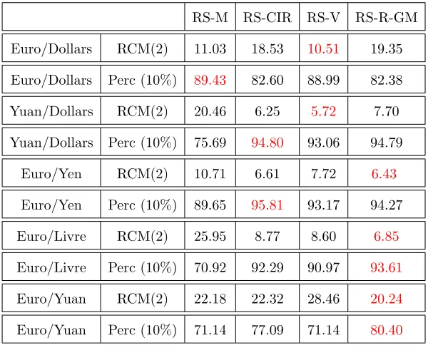
In the following, we evaluate the RCM statistics and the smoothed probability indicators for all foreign exchange rates data and all models. The results are stated in Table 7.
RS-M RS-CIR RS-V RS-R-GM
Euro/Dollars RCM(2) 11.03 18.53 10.51 19.35
Euro/Dollars Perc (10%) 89.43 82.60 88.99 82.38
Yuan/Dollars RCM(2) 20.46 6.25 5.72 7.70
Yuan/Dollars Perc (10%) 75.69 94.80 93.06 94.79
Euro/Yen RCM(2) 10.71 6.61 7.72 6.43
Euro/Yen Perc (10%) 89.65 95.81 93.17 94.27
Euro/Livre RCM(2) 25.95 8.77 8.60 6.85
Euro/Livre Perc (10%) 70.92 92.29 90.97 93.61
Euro/Yuan RCM(2) 22.18 22.32 28.46 20.24
Euro/Yuan Perc (10%) 71.14 77.09 71.14 80.40
Table 7.
RCM statistics and percentage given by the smoothed probability
indicator for 10%:
P
10%.
indicates that the two regimes obtained via the EM-algorithm classify the data in a very good way. And hence, there exists different regimes in the dynamics of foreign exchange rate. Therefore, it is better to take into account the existence of this regime switching in modeling foreign exchange rate dynamics.
3.4. Model fitting. In this subsection, some interesting tests are done to show which is the best regime switching model in the sense that it fits better foreign exchange rate data. For this aim, we evaluate the log likelihood values of each models obtained in the calibration. Thus, a likelihood maximization procedure is used. Furthermore, we calculate the Akaike information criterion (AIC) and the Bayesian information criterion (BIC) which are given by
AIC=−2 ln(L( ˆΘ)) + 2∗k,
and
BIC =−2∗ln(L( ˆΘ)) +kln(n)
whereL( ˆΘ) is the log-likelihood value obtained with the estimated parameters,kis the degree of freedom of each models andnthe number of data for each historical foreign exchange rates.
All the results are stated in Tables 13, 14 and 15 at the end of the paper. The decision rule is the following: Given a set of candidate models for the data, the preferred model is the one with the minimum AIC or BIC value. Hence, we can see from Table 14 and 15, that in all the cases, regime switching models give a less AIC and BIC values than corresponding non regime switching models. This demonstrates that regime switching models fit better the data than non regime switching model. Moreover, Table 13 gives the log likelihood values of each models and it is clear that this value is always higher for regime switching models than non regime switching models. This confirms the previous statement.
Let us now check which is the better regime switching model. To make a choice, we have to take into account two things. Firstly, the log likelihood value given by the model. Indeed, higher in this value and better the fit of the data, better is the model. But, secondly, we have to weight these values with the values given by the (RCM) in Table 7, which measures the good classification of the data. Indeed, even if a model has a higher log likelihood value it is important that its RCM to be close to zero. As an example, if we took the Euro/Yen results, the higher log likelihood value is obtained by the (RS-M) model
The Akaike information criterion is a measure of the relative goodness of fit of a statistical model. It was developed by Hirotsugu Akaike, under the name of ”an information criterion” (AIC), and was first published by Akaike (1974) in [1].
(-1012.42) but this value is closed to the one given by the (RS-V) model (-1015.83). So if comparing their (RCM), we see that (RS-M) model has a (RCM) equals to 10.71 but the (RS-V) has a value equals to 7.72. In conclusion, the choice of the (RS-V) model is better to fit this data since is obtained a log likelihood value close to the best model but obtained a better classification of the regime. Regarding all the results, the choice of the (RS-CIR) or (RS-R-GM) seems to be the best model to fit well data and obtain a good classification of the data with significant regime periods.
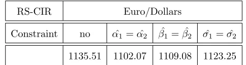
3.5. Impact of regime switching in each parameters. In this section, we would like to see what would happen if one of the three parameters of the model (1.2) do not depend on the regime switching process. To answer this question, we run another simulation and show in Table 8 for the Euro/Dollars foreign exchange rate data and the RS-CIR model, by assuming that one of the parameters don’t depend on the regime switching. This exercise gives a log likelihood value less than the RS-CIR model. This means that the CIR model, where all parameters depend on the regime switching process, fits better to the real data. Therefore, assuming that the speed of adjustment processβ or the volatility parameterσ are equal in each regime give a worse fit on data than in the RS-CIR model.
RS-CIR Euro/Dollars
Constraint no αˆ1= ˆα2 βˆ1= ˆβ2 σˆ1= ˆσ2 1135.51 1102.07 1109.08 1123.25
Table 8.
Log Likelihood value for the RS-CIR model given by
dr
t= (
α
t−
β
tr
t)dt
+
σ
t√
r
tdW
twith two regimes.
Furthermore, similar conclusion can be obtained if we take another foreign exchange rate data or another regime switching model.
3.6. Three Regimes case. One step further from the previous subsections, we would like to see what would be the outcomes if there exist three Markov switching regimes. One could capture “normal” economic dynamics, a second presents for “crisis” and the last one states “good” economic performance. Can more regimes capture more precisely the economic and financial dynamics, what would be the gain and what could be the lost if more regimes are introduced?
Data Statistics RS-M RS-CIR RS-V RS-R-GM
RCM(2) 11.03 18.53 10.51 19.35
RCM(3) - 10.83 13.72 11.00
P10%(2) 89.43 82.60 88.99 82.38 Euro/Dollars
P10%(3) - 90.60 87.22 90.45
RCM(2) 20.46 6.25 5.72 7.70
RCM(3) - 7.57 8.49 13,78
P10%(2) 75.69 94.80 93.06 94.79 Yuan/Dollars
P10%(3) - 93.06 92.13 84.95
RCM(2) 10.71 6.61 7.72 6.43
RCM(3) - 53.53 3.00 7.16
P10%(2) 89.65 95.81 93.17 94.27 Euro/Yen
P10%(3) - 46.92 97.50 93.10
RCM(2) 25.95 8.77 8.60 6.85
RCM(3) - 63.48 61.86 51.09
P10%(2) 70.92 92.29 90.27 93.61 Euro/Livres
P10%(3) - 34.36 35.83 40.31 RCM(2) 22.18 22.32 28.46 20.24
RCM(3) - 44,87 17.40 44.00
P10%(2) 71.14 77.09 71.14 80.40 Euro/Yuan
P10%(3) - 52.64 82.97 54.70
Table 9.
RCM statistics in the case of two and three regimes and percentage
given by the smoothed probability indicator for 10% in the case of 2 and 3 regimes.
It is clear from the Table 9 that the regime classification measure (RCM) is bigger in three regimes cases than in the two regimes case for almost all the data and regime switching models. Moreover, we notice that in many cases the three regimes cases gives very bad classification with respect to the two regimes cases. Indeed, in the case of Euro/Livre, using the (RS-CIR) model, only 34.36% of the data are good classified for 10% error under the three regimes cases against 92.29% with the two regimes cases.
confirmed by the value of the smoothed probability indicator. Indeed, for 10% error, 90.60% of the data are good classified in the 3 regimes model while only 82.60% in the 2 regimes case.
Jan 01 Jan 02 Jan 03 Jan 04 Jan 05 Jan 06 Jan 07 Jan 08 Jan 09 Jan 10 Jan 11 Jan 12May 12 Dates
Jan 01 Jan 02 Jan 03 Jan 04 Jan 05 Jan 06 Jan 07 Jan 08 Jan 09 Jan 10 Jan 11 Jan 12May 12 Dates
Figure 7.
Euro/Dollar foreign exchange rate models with (RS-CIR) with
re-spect to the regime state for: on left: two regimes and on right: three regimes.
As to the Euro/Dollar exchange rate, Figure 7 displays that the three regime case separates better the second regime (in red) than in the two regimes case. The three regimes cases differentiate the two level of the more volatile time periods (the red regime obtained in the two regimes cases): the first one, in green, correspond to the lower value time period and the second one, in red, the higher value time period. Hence, this two periods are differentiate by long mean level value αˆ2
ˆ
β2
= 0.1833
0.1371 = 1.3370 for the regime 2, in red, and αˆ3
ˆ
β3
=00..11531280= 0.9008 for the regime 3, in green. And they have a comparable level of volatility ˆσ2= 0.02617 and ˆσ3= 0.02030 against ˆσ1= 0.01511 for the blue regime.
Jan 01 Jan 02 Jan 03 Jan 04 Jan 05 Jan 06 Jan 07 Jan 08 Jan 09 Jan 10 Jan 11 Jan 12May 12 Dates
Jan 01 Jan 02 Jan 03 Jan 04 Jan 05 Jan 06 Jan 07 Jan 08 Jan 09 Jan 10 Jan 11 Jan 12May 12 Dates
Figure 8.
Euro/Livres foreign exchange rate models with (RS-CIR) with
re-spect to the regime state for: on left: two regimes and on right: three regimes.
As a conclusion, two regimes seems to be the best choice because it gives significant better results in most cases. In the cases where results are better with three regimes, the gain in term of classification is very small regarding the lost in the cases where three regimes give worst results. Hence, it’s better to always take two regimes rather than three.
4. Forecasting
Given observations (rt0, rt1, . . . , rtk) taken at timetk,k∈ {0, . . . , M}, we can define the mean-squared error (MSE) for a given model as
(4.17) M SE= 1
M+ 1 M∑+1
i=1
(ˆrti−rti) 2
where ˆrtiis the predicted value ofrtigiven all information available up to timeti−1(i.e.,F r
ti−1). Moreover,
we recall first that ∆t=ti−ti−1 is a constant and
ˆ
rti+∆t =E
[
rti+∆t|F r ti
]
is a function of rti and the current estimates of all the parameters. By (2.7), the distribution ofrti+∆t is normal with mean
rti+
(
ˆ
αti+1−βˆti+1rti
)
∆t.
Hence, for two state regime switching models, we get
E[rti+∆t|F r ti
]
=π1.(E[rti+∆t|Xti+∆t = 1;F r ti
])
+π2.(E[rti+∆t|Xti+∆t= 1;F r ti
])
.
So, it yields
E[rti+∆t|F r ti
]
=π1.
(
rti+
(
ˆ
α1−βˆ1rti
)
∆t
)
+π2.
(
rti+
(
ˆ
α2−βˆ2rti
)
∆t
)
.
In Table 10, 11 and 12 we display the MSE statistics for ours different models and for each foreign exchange rates data. Keeping the last 60 values of r for the forecast estimation, we estimate all the model parameters using the firstM −60 values ofr. In other words, thisM −60 first data serves as a training data set in order to learn the parameters of each model. Then, starting from theM−60 values, perform the one step ahead, the two step ahead and the three step ahead predictions via using these parameters’ estimation.
Euro/Dollars Yuan/Dollars Euro/Yen Euro/Livre Euro/Yuan
(RS-M) 0.6698×10⁻³ 0.3328×10⁻³ 4.2696 0.1183×10⁻³ 0.0278 (RS-CIR) 0.6839×10⁻³ 0.3131×10⁻³ 4.2648 0.1182×10⁻³ 0.0275
(RS-V) 0.6698×10⁻³ 0.6079×10⁻³ 4.3282 0.1181×10⁻³ 0.0276 (RS-R-GM) 0.6835×10⁻³ 0.3130×10⁻³ 4.3499 0.1180×10⁻³ 0.0275
Table 10.
MSE comparison of each model and data for One Ahead Forcast.
Euro/Dollars Yuan/Dollars Euro/Yen Euro/Livre Euro/Yuan
(RS-M) 0.0012 0.0007 9.6947 0.1992×10⁻³ 0.05
(RS-CIR) 0.0012 0.0006 9.6535 0.1986×10⁻³ 0.049 (RS-V) 0.0012 0.0018 9.9092 0.1982×10⁻³ 0.0489
(RS-R-GM) 0.0012 0.0006 9.9624 0.1978×10⁻³ 0.0489
Table 11.
MSE comparison of each model and data for Two Ahead Forcast.
Euro/Dollars Yuan/Dollars Euro/Yen Euro/Livre Euro/Yuan
(RS-M) 0.0015 0.0009 14.9629 0.2685×10⁻³ 0.0684 (RS-CIR) 0.0016 0.0008 14.8482 0.2669×10⁻³ 0.0663 (RS-V) 0.0015 0.0034 15.4086 0.2662×10⁻³ 0.0669 (RS-R-GM) 0.0016 0.0008 15.4871 0.2651×10⁻³ 0.0660
Table 12.
MSE comparison of each model and data for Three Ahead Forecast.
10 20 30 40 50 60
True Value Predicted Value RS−CIR Predicted Value RS−GBM Predicted Value RS−OU Predicted Value RS−Optimise
Figure 9.
One day forecasting for the Euro/Yuan exchange rate.
5. Conclusion
state spaceS) allows us to highlight some economic and financial time periods where dynamics of foreign exchange rates are significantly different.
Furthermore, we extend the expectation-maximization algorithm, with a filtering and smoothing tech-nique to smooth out noisy data, to calibrate the regime-switching model and show that only a few number of step is needed to obtain a very good calibration. Thus, this refined and modified filtering and smoothing algorithm could be used for other studies and tests of time series related topics, such as the macroeconomic effects of tax changes, different countries bond-stock market, and some more detail can also be found in Romer and Romer (2010).
Conflict of Interests
The authors declare that there is no conflict of interests.
Acknowledgements
We appreciate enormously the valuable discussion in the early stage of this work with Michel Beine, Yin-Wong Cheung, Gautam Tripathi and Rafal Weron. But of course, all eventual mistakes and errors are ours.
References
[1] H. Akaike, A new look at the statistical model identification, IEEE Transactions on Automatic Control 19 (1974) 716-723.
[2] A. Ang, G. Bekaert, Regime switching in interest rates, Journal of Business and Economic Statistics 20 (2002) 163-182.
[3] L. Baele, Volatility spillover effects in european equity markets, Journal of Financial and Quantitative Analysis, 40 (2005).
[4] J. Bai, P. Wang, Conditional markov chain and its application in economic time series analysis, Journal of Applied Econometrics, 26 (2010), 715-734.
[5] H. Baron, G. Baron, Un indicateur de retournement conjoncturel dans la zone euro, Economie et Statistique, No. 359-360 (2002) 101-121.
[6] U. Bergman, J. Hansson, Real exchange rates and switching regimes, Journal of International Money and Finance, 24 (2005) 121-138.
[8] N. Bollen, S. Gray, R. Whaley, Regime switching in foreign exchange rates: Evidence from currency option prices, Journal of Econometrics 94 (2000) 239-276.
[9] L. Calvet, A. Fisher, Multifractal Volatility: Theory, Forecasting, and Pricing, Academic Press (2008).
[10] G. Caporale, N. Pittis, Nominal exchange rate regimes and the stochastic behavior of real variables, Journal of International Money and Finance, 14(3) (1995) 395-415.
[11] K.C. Chan, G.A. Karolyi, F.A. Longstaff, A.B, Sanders, An empirical comparison of alternative models of the short-term interest rate, Journal of Finance. 47 (1992) 1209-1227.
[12] Y. Cheung, M. Chinn, A. Pascual, Empirical exchange rate models of nineties: Are any fit to survive?, Journal of International Money and Finance 24 (2005) 1150-1175.
[13] Y. Cheung, U. Erlandsson, Exchange rate and Markov switching Dynamics, Journal of Business and Economic Statistic, 23 (2005) 314-320.
[14] S. Choi, Regime-Switching Univariate Diffusion Models of the Short-Term Interest Rate, Studies in Nonlinear Dynamics & Econometrics, 13 (2009) 4.
[15] S. Choi, M. Marcozzi, The valuation of foreign currency option under stochastic interest rates, Computers and Mathematics with Applications 46 (2003) 741-749.
[16] J. Cox, J. Ingersoll, S. Ross, A theory of term structure of interest rates, Econometrica 53 (1985) 385-407.
[17] R. Dacco, S. Satchel, Why do regime-switching models forecast so badly?, Journal of Forecasting, 18 (1999) 1-16.
[18] A.P. Dempster, N. Laird, D. Rubin, Maximum likelihood from incomplete data via the EM algorithm, Journal of the Royal Statistical Society. Series B (Methodological) 39 (1977) 1-38.
[19] J. Driffill, T. Kenc, The effects of different parameterizations of Markov-switching in a CIR model of bond pricing, Studies in Nonlinear Dynamics and Econometrics, 13 (2009) 1-22.
[20] C. Engle, J.D. Hamilton, Long swings in the Dollar: Are they in the data and do markets know it?, American Economic Review 80 (1990) 689-713.
[21] C. Engle, Can the Markov switching model forcase exchange rates?, Journal of International Eco-nomics, 36 (1994) 151-165.
[22] C. Engle, C. Hakkio, The distribution of exchange rates in the EMS, International Journal of Finance and Economics 1 (1996) 55-67.
[23] L. Ferrara, The contribution of cyclical turning point indicators to business cycle analysis, Banque de France, Quarterly Selection of Articles, 13 (2008).
[25] S. Goutte. Conditional Markov regime switching model applied to economic modelling. Preprint (2012).
[26] S. Goutte. Quadratic regime switching term structures models. Preprint (2013).
[27] G. Schwarz, Estimating the dimension of a model. Annals of Statistics 6 (1978) 461?64.
[28] D.R. Heath, A. Morton, Bond pricing and the term structure of interest rates: A new methodology for contingent claim valuation, Econometrica 60 (1992) 77-105
[29] J. Hamilton, A new approach to the economic analysis of non-stationary time series and the business cycle, Econometrica, 57 (1989a) 357-384.
[30] J. Hamilton, Rational-expectations econometric analysis of changes in regime, Journal of Economic Dynamics and Control, 12 (1989b) 385-423.
[31] B.E. Hansen, The likelihood ratio test under nonstandard conditions: Testing the Markov switching model of GNP, Journal of Applied Econometrics, 7 (1992) 61-82.
[32] J. Janczura, R. Weron, Efficient estimation of Markov regime-switching models: An application to electricity spot prices, Adv. Stat. Anal. 96 (2012) 385-407.
[33] C.J. Kim, Dynamic linear models with Markov-switching, Journal of Econometrics 60 (1994) 1-22. [34] Z. Kontolemis, Analysis of the US business cycle with a Vector-Markov-Switching model, Journal of
Forecasting, 20 (2001) 47-61.
[35] J. Lopez, Exchange rate cointegration across central bank regimes shifts, Federal Reserve Bank of New York Research Article ID 9602 (1996).
[36] N.C. Mark, Exchange rates and fundamentals: Evidence on long-horizon predictability, American Economic Review, 85 (1995) 201-218.
[37] I.W. Marsh, High-frequency Markov switching models in the foreign exchange market, Journal of Forecasting 19 (2000) 123-134.
[38] M. McConnel, G. Perez-Quiros, Output fluctuations in the United States: what has changed since the eearly 1980s?, American Economic Review 90 (2000) 1464-1476.
[39] A. Naszodi, Exchange rate dynamics under state-contingent stochastic process switching, Journal of international Money and Finance, 30 (2011) 896-908.
[40] M.T. Ismail, Z. Isa, Detecting regime shifts in Malaysian exchange rates, Journal of Fundamental science 3 (2007) 211–224.
[41] R. Meese, K. Rogoff, Empirical exchnage rate models of the seventies: Do they fit out of sample?, Journal of International Economics 14 (1983) 3-24.
[43] B. Rossi, Optimal tests for nested model selection with underlying parameter instability, Econometric theory 21 (2005) 962-990.
0 10 20 30 40 50 60 70 80 −0.02
0 0.02
0.04 Alpha
Regime 1 Regime 2
0 10 20 30 40 50 60 70 80 −0.02
0 0.02 0.04
Beta
Regime 1 Regime 2
0 10 20 30 40 50 60 70 80 0.01
0.015 0.02 0.025
Sigma
Regime 1 Regime 2
0 10 20 30 40 50 60 70 80 90 100 −0.05
0 0.05
Alpha
Regime 1 Regime 2
0 10 20 30 40 50 60 70 80 90 100 −10
−5 0 5x 10
−3 Beta
Regime 1 Regime 2
0 10 20 30 40 50 60 70 80 90 100 0
200 400 600
Sigma
Regime 1 Regime 2
0 10 20 30 40 50 60 70 80 90 100 −5 0 5 10 15 Alpha Regime 1 Regime 2
0 10 20 30 40 50 60 70 80 90 100 −0.05 0 0.05 0.1 0.15 Beta Regime 1 Regime 2
0 10 20 30 40 50 60 70 80 90 100 0 10 20 30 Sigma Regime 1 Regime 2
0 10 20 30 40 50 60 70 80 0 0.01 0.02 0.03 0.04 Alpha Regime 1 Regime 2
0 10 20 30 40 50 60 70 80 −0.02 0 0.02 0.04 Beta Regime 1 Regime 2
0 10 20 30 40 50 60 70 80 0 0.01 0.02 0.03 Sigma Regime 1 Regime 2
Figure 11.
Evolution of the calibrated parameters values: on left: Euro/Yen
and on right: Euro/Livres.
0 10 20 30 40 50 60 70 80 90 0 0.1 0.2 0.3 0.4 Alpha Regime 1 Regime 2
0 10 20 30 40 50 60 70 80 90 0.01 0.02 0.03 0.04 0.05 Beta Regime 1 Regime 2
0 10 20 30 40 50 60 70 80 90 0 0.5 1 1.5 Sigma Regime 1 Regime 2
0 50 100 150 200 250 300 350 400 Filtered Probability
Regime 1 Regime 2
0 50 100 150 200 250 300 350 400 Smoothed Probability
Regime 1 Regime 2
0 50 100 150 200 250 Filtered Probability
Regime 1 Regime 2
0 50 100 150 200 250 Smoothed Probability
Regime 1 Regime 2
0 50 100 150 200 250 300 350 400 Filtered Probability
Regime 1 Regime 2
0 50 100 150 200 250 300 350 400 Smoothed Probability
Regime 1 Regime 2
0 50 100 150 200 250 300 350 400 Filtered Probability
Regime 1 Regime 2
0 50 100 150 200 250 300 350 400 Smoothed Probability
Regime 1 Regime 2
Figure 14.
Smoothed and Filtered probabilities for: on left: Euro/Yen and on
right: Euro/Livres.
0 50 100 150 200 250 300 350 400 Filtered Probability
Regime 1 Regime 2
0 50 100 150 200 250 300 350 400 Smoothed Probability
Regime 1 Regime 2