Numerical Simulation of Crack Modeling using Extended Finite Element Method

Numerical Simulation of Crack Modeling using Extended

Finite Element Method

Gordana Jovičić - Miroslav Živković - Nebojša Jovičić

University of Kragujevac, Faculty of Mechanical Engineering, Serbia

For numerical simulation of crack modeling in Fracture Mechanics the eXtended Finite Element Method (X-FEM) has recently been accepted as the new powerful and efficiency methodology. Following the new approach, a discontinuous function and the asymptotic crack-tip displacement functions are added to the conventional finite element approximation. This enables the domain to be modeled by finite elements with no explicit meshing of the crack faces. In the paper we present the details of implementation of the X-FEM algorithm in our in-house finite elements based software. Also, we investigated the impact of the node enrichment variations on results of the developed numerical procedure. In order to evaluate computational accuracy, numerical results for the Stress Intensity Factors (SIF) are compared with both theoretical and conventional finite element data. For the calculation of the Stress Intensity Factors, we used the J-Equivalent Domain Integral (J-EDI) Method. Computational geometry issues associated with the representation of the crack and the enrichment of the finite element approximation are discussed in detail. Obtained numerical results have shown a good agreement with benchmark solutions.

© 2009 Journal of Mechanical Engineering. All rights reserved.

Keywords: extended finite element method, node enrichment, stress intensity factor, j-equivalen domain integral method

0 INTRODUCTION

The X-FEM, attempts to improve computational challenges associated with mesh generation by not requiring the finite element mesh to conform to cracks, and in addition, provides using higher-order elements or special finite elements without significant changes in the formulation. The basis of the method proposed by Belytchko and Black [1], was presented in [2] for two-dimensional cracks.

The essence of the X-FEM lies in sub-dividing the model problem into two distinct parts: mesh generation for the geometric domain (cracks not included), and enriching the finite element approximation by additional functions that model the flaw(s) and other geometric entities. Modeling damage and crack growth in a traditional finite element framework [3] and [4] is cumbersome due to the need for the mesh to match the geometry of the discontinuity. Many methods require remeshing of the domain at each time step. In the X-FEM there is no need for the remeshing, because the mesh is not changed as the crack growths and is completely independent of the location and geometry of the crack. The discontinuities across the crack are modeled by

1 LEVEL SET REPRESENTATION OF THE CRACK

In this paper a crack is presented using a set of the linear segments. The crack is described by means of the tip position and level set of a vector valued mapping. A signed distance function ψ( )x is defined over computational domainΩ using:

* *

x

(x) n (X X ) min X X

c

sign

ψ

∈Γ

⎡ ⎤

= _⎣ ⋅ − _⎦ −

,

where n is the unit normal to Γ_c and _{X is the} *

closest point to the X, see Fig. 1.

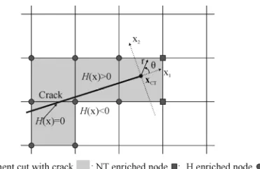
Fig. 1. Illustration of the values of Heavisade function above and below of the crack

The crack is then represented as the zero

ψ(X) =0. (2) The position related to the crack tip is defined through the following functions:

γ(X) = (X -XCT)⋅t, (3)

where t is the unit tangent to ΓC at the crack tip

ΛC and XCT is the coordinate of ΛC. The value

γ(X) = 0 corresponds to the crack tip. We defined LS functions ψ(X) and γ(X) in all the computational domain. The crack and the crack tip are represented as:

{

}

c ψ t γ t

Γ = = ∧ ≤ . (4)

Fig. 2. Definition of the Level Set Functions ψ(X) and γ(X) around the crack

In Fig. 2, definition of the ψ(X) and γ(X) around the crack is shown. For the crack representations linear interpolation has been used.

2 EXTENDED FINITE ELEMENT METHOD

In this paper, the method of discontinuous enrichment is presented in general framework. We illustrate how 2D formulation can be enriched for crack modeling. The concept of incorporating local enrichment in the finite element partition of unity was introduced in Melenk and Babuska [5]. The essential feature is multiplication of the enrichment functions by nodal shape functions.

The displacement approximation u(x) in the X-FEM is decomposed into a continuous and enrichment part, as:

con enrh

u(x) u (x) u= + (x). (5)

The second addond in Eq. 5 is:

N M

h α

enrh I α I

I 1 α 1

u (x) N (x) F (x) b

= =

⎛ ⎞

= _{⎜ ⎟}

⎝ ⎠

∑

∑

where: the continuous displacement approximation h

con I I

u (x)= ∑ N (x)u is standard approximation in the FEM, and u_enrh(x) is enrichment part of displacement approximation near the crack, (Fig. 3). The NI, I = (1, N) are the

finite element shape functions, Fα(x), α = (1, M)

are the enrichment functions and α

I

b is the nodal enriched degree of freedom vector associated with the elastic asymptotic crack-tip function that has the form of the Westergaard field for the crack tip.

2.1. Enrichment Functions

The enrichment is able to take a local form only by enriching those nodes whose support intersects a region of crack. Two distinct regions are identified for the crack geometry, precisely, one of them is the crack interior and the other is near tip region as it is shown in Fig. 3. In Fig. 3 a region of a crack for enrichment by H and NT functions is shown. The circled nodes are enriched with a discontinuous function, while the squared nodes are enriched with NT functions. It can be noticed that this shape of enriching near the crack tip ( Fig. 3), is used in [6] and [7].

Fig. 3. Regions for the standard enrichment near the edges of the crack

* 1 if (X X ) n 0 (X)

* 1 if (X X ) n 0

H = ⎨⎧⎪ − ⋅ ≥

⎪ − − ⋅ <

⎩

, (7)

where X is a sample (Gauss) point, X*_{(lies on the}

crack) is the closest point to X, and n is unit outward normal to crack at X* _{(Fig. 1). It can be}

seen that in the first published works [1] and [2] above shape modeling of the discontinuity was not used. The formulation (7) begins to use it due to practical numerical reasons.

The crack tip enrichment functions in isotropic elasticity have the form of the Westergaard field for the crack tip:

1 2 3 4

( ) { , , , }

cos , sin , sin sin ,

2 2 2

cos sin 2

F F F F F

r r r

r θ θ θ _θ θ _θ = = ⎡ ⎤ ⎢ ⎥ ⎢ ⎥ ⎢ ⎥ ⎢ ⎥ ⎣ ⎦ x , (8)

where is r and θ denotes polar coordinates in the locale system at the crack tip. It can be noted that the second function of the set (8) is discontinued over the crack faces [1] and [2]. The discontinuity over the crack faces can be obtained using other functions like Heavisade function (7), which have discontinuity. Let the element which contains the crack tip is denoted as CT element. In papers [6] and [7] the discontinuity behind the tip in the CT element is accomplished by the second function of the set (8). In this paper we have achieved the discontinuity in the CT element with Heavisade function (7).

The Heavisade step function (7) is modified using LS function γ (X, t):

1 if (X) 0 ( (X))

1 if (X) 0

H γ γ

γ

− <

⎧

= ⎨_{+ >}

⎩ . (9)

The Near tip functions Fα(r, θ), α = 1.4,

that have the form of the Westergaard field for the crack tip [5], should also be defined using the LS functions [8] to obtain polar coordinates in the local system at the crack tip (see Fig. 3):

2 2

1

(X) (X) (X) , (X) (X) tan .

(X)

r ψ γ

γ θ ψ − = + = (10)

Since NT functions are used for the cracks in the linear-elastic materials, we have considered the results in case when the enricment is done only by H function. Enrichment by H function is applied only behind the crack, hence discontinuity is occured.

3 DETERMINATION OF THE SIF USING J-EDI METHOD

The contour J-integral [9] is not in the best-suited form for finite element calculations. Therefore, we transform the contour integral into an equivalent domain form. The equivalent domain integral method (EDI) is an alternative way to obtain the J-integral. The EDI approach has the advantage in that the effect of body forces can be included very easily. The contour integral is replaced by an integral over a finite-size domain, [10] to [12]:

(

)

1 A ij i,1 1j ,j , 1, 2

J =∫ σ u −Wδ q dA i j= , (11)

where W is the strain energy density given by:

1 1

2 ij ij 2 ijkl kl ij

W = σ ε = C ε ε , (12)

where: σij is stress tensor, εij is strain tensor, Cijkl

is constitutive tensor, ui are components of the

displacement vector, where the qj is the derivate

of the weight function per coordinates x. With the isoparametric finite element formulation the distribution of q within the elements is determined by a standard interpolation scheme with the use of the shape functions NI.The spatial

derivatives of q can be found by the use of the usual procedures for isoparametric elements.

The equivalent domain integral in 2D can be calculated as a sum of the discretized values of Eq. (11), [10] to [13]:

1

det

i

ij kj

P _{k j}

k p elements p m in A n _p u q W X X J w X σ δ η = ⎡⎛ ∂ ⎞ ∂ ⎤ − ⎢⎜ _∂ ⎟_∂ ⎥ ⎝ ⎠ ⎢ ⎥ = ∑ ∑ ⎢ _{⎛∂ ⎞} ⎥ ⎢_{⋅ ⎜ ⎟} ⎥ ⎢ _⎝∂ _⎠ ⎥ ⎣ ⎦

,

, , , , 1, 2

i j k m n=

.

(13)

The terms within [.]p are evaluated at the

body forces are present. The J-integral evaluation in this paper is used for the calculation of SIF in both FEM and X-FEM frameworks.

4 NUMERICAL EXAMPLES

In Fig. 4, a benchmark plate model with an edge crack is shown. The plate is subjected to load along the crack faces. Both, geometrical as well material data for test case are presented in Fig. 4. Numerical calculations of SIF are carried out by using the X-FEM method, with the H and H+NT enrichment options. Obtained numerical results are compared to the theoretical values.

E = 3⋅106 _{MPa, v = 0.29, a = 20 mm} P = 1 N, W = 40 mm, s = 80 mm, B = 0.5 mm

Fig. 4. The edge crack subject to the concentration load along the face of the crack

Within the X-FEM calculations, the numerical grid consisting of 1600 elements (80⋅20) was used. The simulation of the discontinuous displacement field on the crack sides, as well singularly stress field near the crack tip, are performed by using the enrichment functions.

Theoretical values of SIF can be calculated as follows:

I

2 ( s a, )

K F a

W W σ π

= , (14)

where

2

6 6 2

M Ps

BW W

σ = = . (15)

The correction factors for the specified geometrical parameters (2 s/W = 4 and a/W = 0.5) are F(2 s/W, a/W) = 1.41, while σ = 0.3 MPa. Theoretical value of SIF for the test case is:

teor

I 3.35 MPa mm

K = . (16)

The simulations were performed within two versions of the presented numerical algorithms:

− Nodes are enriched by only using the H function (XFEM (H));

− Nodes are enriched by using the H+NT function (XFEM (H+NT)).

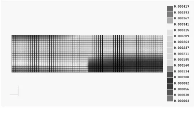
In Figs. 5 and 6, both, the stress and strain field around the crack, obtained by using the X-FEM, are shown, respectively. The crack overlaps the element edges, and there is no physical separation of the joint sides of the elements. In this case, the discontinuity at the crack faces is modeled by using enrichment functions. In Fig. 5, it can be noticed that within the extended X-FEM framework the stress concentration is located well, i.e., placed at the real crack tip. The displacement field around the central crack obtained by extended X-FEM is shown in Fig. 6. It is worth stressing that we have obtained discontinuity in the displacement field over the crack faces by using the Heavisade function, without explicitly geometrical crack modeling.

In Table 1, values of SIF for the number of the integration domains are shown. These values are obtained by using the X-FEM, with the H, as well H+NT enrichment in the nodes that are cut by crack. The results for the SIF are shown in Table 1, obtained by the integration of the J -integral using the J-EDI method, corresponding to the different integration domainr_c. The radius of the integration domain rcis defined as % of the

length of the cracka.

Table 1. The SIF corresponding to the different integration domain obtained by the H and H+NT enrichment

rc

(% a) 30 35 40 45 50 55 60 65

KI

XFEM

(H) 3.22 3.22 3.24 3.26 2.92 3.28 3.29 3.31 KI

XFEM

(H+NT)3.26 3.25 3.27 3.29 3.29 3.29 3.29 3.29

Comparing the numerical data with the theoretical results, it can be noticed that the error was 4%≤ for the case of the H enrichment. With using the H+NT enrichment, discrepancy was

3%

variation in the results, obtained by both approaches, is relativelysmall. On the other hand, a decrease in error for the numerical results of SIF could be achieved by grid refinement, particularly in the location of the crack tip.

Fig. 5. The stess field arround the model with the edge crack

Fig. 6. The displacement field arround the model with the edge crack

5 CONCLUSION

The essential idea in the X-FEM method is to add enrichment functions to the approximation that contains a discontinuous displacement field. The crack is presented as discontinuity in displacements within the element. The X-FEM does not require projection between mesh and crack geometry, and allows arbitrary crack in the finite element mesh.

In this paper we demonstrated the modeling of enriched nodes near the crack within an existing finite element numerical algorithm. The methodology adopted for the crack modeling belongs to a branch of the extended finite element method (X-FEM). The developed finite element software was used in this study, and the

isotropic media was described. The crack is described by means of the position of the tip and level set of a vector valued mapping. In this paper, the developed LS functions are used to determine the values of the NT functions. We also modified the enriching of the corresponding elements. Numerical results obtained in this way are compared with the theoretical values, and good agreement is achieved. This study presents the wide capability of the X-FEM approach that can be incorporated in standard finite element packages.

6 REFERENCES

[1] Belytschko, T., Black, T. (1999) Elastic crack growth in finite elements with minimal remeshing, International Journal for Numerical Methods in Engineering, vol.45, no.5, p. 601-620.

[2] Moes, N., Dolbow, J., Belytschko, T. (1999) A finite element method for crack growth without remeshing, International Journal for Numerical Methods in Engineering, vol. 46, no. 1, p. 131-150.

[3] Rosa, U., Nagode, M., Fajdiga, M. (2007) Evaluating thermo-mechanically loaded components using a strain-life approach,

Strojniški vestnik - Journal of Mechanical Engineering, vol.53, no. 10, p.706-71

[4] Vrh, M., Halilovič, M. (2008) Impact of young's modulus degradation on springback calculation in steel sheet drawing, Strojniški vestnik - Journal of Mechanical Engineering

vol. 54, no. 3, p. 288-296.

[5] Melenk, J.M., Babuska, I. (1996) The partition of unity finite element method: Basic theory and applications, Computer Methods in Applied Mechanics and Engineering, vol. 39, p. 289-314.

[6] Daux, C., Moes, N., Dolbow, J., Sukumur, N., Belytschko, T. (2000) Arbitrary cracks and holes with the extended finite element method, International Journal for Numerical Methods in Engineering, vol. 48, no. 12, p. 1741-1760.

7513-[8] Jovičić G. (2005) An extended finite element method for fracture mechanics and fatigue analysis, (in Serbian), Ph.D. thesis,

University of Kragujevac.

[9] Sedmak, A. (2003) Applicatiion of fracture mechanics to the structural integrity (in Serbian), University of Belgrade.

[10] Rice, J.R. (1968) A path independent integral and approximate analysis of strain concentration by notches and cracks, Journal of Applied Mechanics, vol. 35, p. 379-386. [11] Lin C.Y. (2000) Determination of the

Fracture Parameters in a Stiffened Composite Panel, Ph.D. thesis, North Carolina State University.

[12] Kim, J.H., Paulino, G.H. (2002) Mixed-mode J-integral formulation and implementation using graded elements for fracture analysis of no homogeneous orthotropic materials, Mechanics of Materials, vol. 35, p. 107-128.

[13] Enderlein, M., Riceour, A., Kuna, M. (2003) Comparison of finite element techniques for 2D and 3D crack analysis under impact loading, International Journal of Solids and Structuresc, vol. 40, p. 3425-3437.

[14] Kojic, M., Jovicic, G., Zivkovic, M., Vulovic, S. (2004) Numerical programs for life assessment of the steam turbine housing of the thermal power plant, Special Issue: From Fracture Mechanics to Structural Integrity Assessment, University of Belgrade. [15] Kojić, M., Jovičić, G., Živković, M.,

Vulovic, S. (2005) PAK-FM&F - software for fracture mechanics and fatigue based on the FEM and X-FEM, Manual, University of Kragujevac.

[16] Knez, M., Kramberger, J., Glodez, S. (2007) Determination of the low-cycle fatigue parameters of S1100Q high-strength steel,