www.the-cryosphere.net/5/989/2011/ doi:10.5194/tc-5-989-2011
© Author(s) 2011. CC Attribution 3.0 License.
The Cryosphere
The multiphase physics of sea ice: a review for model developers
E. C. Hunke1, D. Notz2, A. K. Turner1, and M. Vancoppenolle3 1Los Alamos National Laboratory, Los Alamos, New Mexico, USA 2Max Planck Institute for Meteorology, Hamburg, Germany
3Georges Lemaˆıtre Centre for Earth and Climate Research, Universit´e Catholique de Louvain, Louvain-la-Neuve, Belgium Received: 23 June 2011 – Published in The Cryosphere Discuss.: 22 July 2011
Revised: 27 October 2011 – Accepted: 31 October 2011 – Published: 14 November 2011
Abstract. Rather than being solid throughout, sea ice con-tains liquid brine inclusions, solid salts, microalgae, trace elements, gases, and other impurities which all exist in the interstices of a porous, solid ice matrix. This multiphase structure of sea ice arises from the fact that the salt that ex-ists in seawater cannot be incorporated into lattice sites in the pure ice component of sea ice, but remains in liquid so-lution. Depending on the ice permeability (determined by temperature, salinity and gas content), this brine can drain from the ice, taking other sea ice constituents with it. Thus, sea ice salinity and microstructure are tightly interconnected and play a significant role in polar ecosystems and climate. As large-scale climate modeling efforts move toward “earth system” simulations that include biological and chemical cy-cles, renewed interest in the multiphase physics of sea ice has strengthened research initiatives to observe, understand and model this complex system. This review article provides an overview of these efforts, highlighting known difficulties and requisite observations for further progress in the field. We focus on mushy layer theory, which describes general mul-tiphase materials, and on numerical approaches now being explored to model the multiphase evolution of sea ice and its interaction with chemical, biological and climate systems.
1 Introduction
Biologists in the polar regions face an apparent contradic-tion: the bulk salinity of sea ice (around 5 ppt) is consider-ably smaller than that in the underlying polar oceans (around 32 ppt) – salty brine drains from sea ice – and yet chlorophyll concentrations in sea ice (a measure of microalgal biomass) can be two orders of magnitude larger than in the surrounding
Correspondence to: E. Hunke
ocean (Arrigo et al., 1997). How do these organisms and the nutrients they need to survive reach such high concentrations, while the brine drains? This question, and its potential im-pact on polar ecosystems and climate, motivates a relatively new thrust in global-scale sea ice research that aims to under-stand and model the multiphase physics of sea ice. Indeed, the desalination mechanisms themselves are not well under-stood. In this review, we will give an overview of the recent advances in our understanding of the multiphase physics of sea ice. We will also describe how these advances are cur-rently guiding the development of new sea-ice models which allow for an improved simulation of the interaction of sea ice with the ocean and the atmosphere.
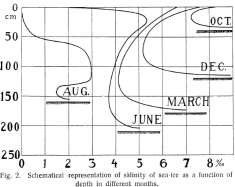
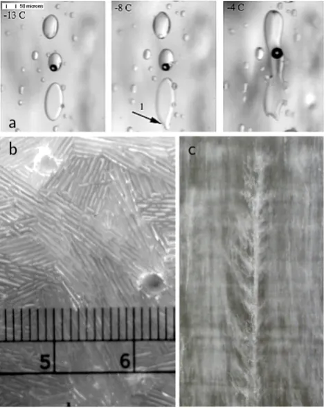
Sea ice salinity has long fascinated sea ice researchers for the complexity that it produces through depression of freez-ing and meltfreez-ing temperatures. Malmgren (1927) discussed the evolution of the vertical salinity profile, illustrated in Fig. 1, and recognized its effect on the thermal properties of sea ice. As sea water freezes, salt becomes concentrated in interstitial liquid brine inclusions. Because phase equilib-rium must be maintained between these inclusions and the surrounding ice, the salt becomes more and more concen-trated as temperatures decrease. Solid salts begin to precipi-tate out of solution, starting with CaCO3at−2.2◦C, NaSO4 (the mineral Mirabilite) at−8.2◦C and NaCl at−23◦C. Fig-ure 2 shows the phase diagram of sea ice as determined by Assur (1958) (see chapter 6 of Weeks (2010) for a com-plete description of the phase diagram). During periods of warming, some fresh ice dissolves in the liquid brine, ex-panding the brine inclusions, as shown in Fig. 3a. As sea ice ages, much of the liquid brine is lost from the ice, primarily through downward convection in vertical brine channels that form naturally during sea-ice formation (Fig. 3b, c).
Fig. 1. Malmgren’s (1927) diagram of sea ice salinity, as a
func-tion of depth for 5 different months, also illustrates the evolufunc-tion of sea ice thickness during the annual cycle. As Malmgren notes, this figure “is intended only to give a qualitative picture of the course of development and the salinities must not be interpreted as repre-senting the mean values of the salinity during the different months.” Reprinted from Malmgren (1927).
1992), probably due to intense rafting, surface flooding and snow ice formation. Eicken’s (1992) ice-core based classifi-cation of ice salinity profiles (Fig. 4) features typical profiles that differ significantly from their Arctic counterparts. C-type profiles, such as those found for winter Arctic first-year ice, appear but are not prevalent (25 % of the profiles). The most abundant profiles had high salinities (>10 ppt) near the surface (S-type, 51 %), which Eicken associated with sea-water flooding and snow ice formation. Profiles with low salinity values near the surface were not as frequent (16 %) as in the Arctic, where they are ubiquitous in summer, likely associated with the lack of surface melt in austral summer (Andreas and Ackley, 1982). Furthermore, 7 % of the pro-files were found to be nearly isosaline (I-type). Although the seasons were not evenly sampled, Eicken’s classification pro-vides a general idea of the salinity profile in Antarctic sea ice. Notably, very little difference between first-year and multi-year salinity profile shapes is observed, as pointed out by Eicken (1998) in a later study using essentially the same data set. Furthermore, Haas et al. (2001) and Ackley et al. (2008) note that the heavy snow layer present in the Antarctic may encourage superimposed ice formation as well as the occur-rence of liquid gap layers at the snow-ice interface, providing yet more diversity in Southern Hemisphere sea ice salinity profiles.
Other constituents in the sea water, such as algae and bac-teria, can exist in the interstices of the solid matrix, along with the salt. Communities of these organisms form within the ice, their life cycles largely determined by penetrating sunlight and by fluxes of nutrients between the ocean and
Fig. 2. The phase diagram for sea ice from Assur (1958). Open
squares show the temperature at which the labeled solid salts be-gin precipitating according to the experiments of Nelson (1953) and Nelson and Thompson (1954). Adapted and reprinted with permis-sion from “Arctic Sea Ice”, 1958, by the National Academy of Sci-ences, courtesy of National Academies Press, Washington, DC.
ice. The nutrient fluxes are, in turn, controlled by the porous ice structure that depends critically on the temperature and salinity of the ice. For example, cold or warm fronts pass-ing vertically through the ice after the onset of storms cause the brine inclusions to contract or expand, thus altering the permeability. When the ice becomes impermeable, nutrient fluxes cease and primary productivity within the ice declines (Fritsen et al., 1994).
Fig. 3. (a) Warming sequence showing changes in ice structure at −13◦C,−8◦C, and−4◦C. The arrow in the center panel indicates merged brine inclusions, and the three large inclusions have merged in the third panel. The vapor bubble at the center of the image also expands in size as the sample warms (Light et al., 2003, used with permission, American Geophysical Union). (b) Laboratory-grown sodium-chloride ice showing horizontal crystalline structure and 2 brine channel openings at the bottom of the ice (compare Wettlaufer et al., 1997b). (c) Brine channel in a vertical slab of Arctic sea ice (pictured height approximately 60 cm; photo: H. Eicken).
et al., 2011). In addition, for reasons that are not yet fully understood, particulate and dissolved iron accumulate in sea ice (e.g., Lannuzel et al., 2010; van der Merwe et al., 2011), while all other impurities have smaller concentrations in sea ice than in seawater. Understanding why iron accumulates in sea ice depends on a better understanding of sea ice multi-phase physical processes and how they interact with biogeo-chemical processes. The storage and transport of iron associ-ated with sea ice dynamics is important because it may stimu-late summer phytoplankton blooms in the Southern Ocean, as shown by a preliminary model investigation of the Southern Ocean (Lancelot et al., 2009). Overall, the sea-ice habitat ap-pears to be highly productive and is thought to make a signif-icant contribution to the carbon, sulfur and iron cycles, which needs to be carefully assessed. Previous assessments of the impact of sea ice on the large-scale carbon cycle suffer from uncertainties in observed and simulated primary production
in sea ice (Legendre et al., 1992; Arrigo et al., 1997; Zem-melink et al., 2008). Indeed, fundamental chemical equilibria at subzero temperatures are not well understood for aqueous geochemical processes as in sea ice (Marion, 2001).
Generally speaking, large-scale models, such as those used for regional or global climate simulations, can not simulate the detailed physical structures of brine inclusions, whose scales range from the sub-millimeter to around 1 cm in di-ameter. (Channels may stretch the full depth of the ice, however.) Ice models traditionally treat thermodynamic pro-cesses, including those dependent on salinity such as ther-mal conductivity, in a one dimensional, horizontally aver-aged sense. The thermodynamic model of Maykut and Un-tersteiner (1971) and its variants (Semtner, 1976; Bitz and Lipscomb, 1999; Winton, 2000) have generally sufficed for global climate modeling purposes, but GCMs are now begin-ning to include complex ecosystem models in order to more fully capture the carbon cycle, for instance. While sea ice was considered primarily a barrier between atmosphere and ocean for biogeochemically relevant fluxes, its influence on the ecosystems and chemistry in the polar regions is now be-coming recognized and sea ice researchers are striving to im-prove representations of sea ice multiphase physics in mod-els.
Such improved representation has in the past been hin-dered by a lack of understanding of fundamental processes driving the evolution of sea-ice microstructure. Hence, most current sea-ice models do not allow for a realistic simula-tion of the evolusimula-tion of sea-ice salinity, solid fracsimula-tion, and the transport of biogeochemical tracers within the ice. Recently, a theoretical framework to handle other such complex, mul-tiphase materials, mushy layer theory, has been applied to sea ice (Taylor and Feltham, 2004; Oertling and Watts, 2004; Notz and Worster, 2006; Petrich et al., 2007). Mushy layer theory consists of a proper formulation of energy, mass and solute conservation equations. Through the application of mushy layer theory to sea ice, we now have a solid physical basis on which future parameterizations of the interior struc-ture of sea ice can be based. An introduction to this theory, focusing on its applicability to sea ice, is given in Sect. 2. In Sect. 3, we provide an overview of the history of sea-ice models, focusing on their approximations of multiphase physics, and we outline how the future development of sea-ice models can profit from parameterization implementations based on mushy layer theory. Finally, in Sect. 4 we outline pertinent observational studies, highlighting needs for sea ice multiphase modeling.
2 Basic physics
(a) (b)
(c) (d)
Fig. 4. Classification of Antarctic sea ice salinity profiles proposed by Eicken (1992) based on 129 cores from the Weddell Sea taken during
four campaigns in the 1980s. (a) C-type, 33 profiles, (b) S-type, 66 profiles, (c) ?-type, 21 profiles, (d) I-type, 9 profiles. The different curves refer to the composite salinity profile (solid), compositeδ18O profile (dotted line), actual data for one particular salinity profile (circles), and a polynomial associated with the specific salinity profile (dash) (Eicken, 1992, reprinted with permission, American Geophysical Union).
fraction of solid ice (or the fraction of liquid brine, respec-tively). These parameters are closely related, and it is usually sufficient to know any two of them in order to calculate the third. The relationship between these parameters can easily be seen by considering, for example, the bulk salinitySthat describes the salinity of a melted sea ice sample. Denoting the fraction of solid ice asφ, the bulk salinity can be written as
S=φSice+(1−φ)Sbr(T ). (1)
Here,Sbr denotes the salinity of the interstitial liquid brine, whileSiceis the salinity of the solid ice lattice, with salinity defined as g salt per kg brine (or ice, or bulk material),
de-noted as ppt. (All symbols used in the text are defined in Ta-ble 1.) Since salt ions are not incorporated into the ice crystal lattice other than in trace amounts,Sice=0, and Eq. (1) can be rewritten as
(1−φ)= S Sbr(T )
. (2)
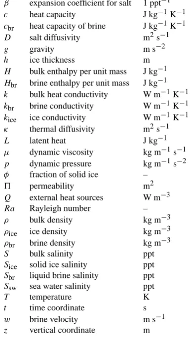
Table 1. Symbols, used in the text, with their definitions and units.
β expansion coefficient for salt 1 ppt−1
c heat capacity J kg−1K−1
cbr heat capacity of brine J kg−1K−1 D salt diffusivity m2s−1
g gravity m s−2
h ice thickness m
H bulk enthalpy per unit mass J kg−1
Hbr brine enthalpy per unit mass J kg−1 k bulk heat conductivity W m−1K−1
kbr brine conductivity W m−1K−1 kice ice conductivity W m−1K−1
κ thermal diffusivity m2s−1
L latent heat J kg−1
µ dynamic viscosity kg m−1s−1
p dynamic pressure kg m−1s−2
φ fraction of solid ice –
5 permeability m2
Q external heat sources W m−3
Ra Rayleigh number –
ρ bulk density kg m−3
ρice ice density kg m−3 ρbr brine density kg m−3 S bulk salinity ppt
Sice solid ice salinity ppt Sbr liquid brine salinity ppt Ssw sea water salinity ppt T temperature K
t time coordinate s
w brine velocity m s−1
z vertical coordinate m
Because the interstitial brine is surrounded by solid fresh-water ice, phase equilibrium must always be maintained be-tween these two phases. Hence, volume and salinity of the brine inclusions adjust in order to maintain the tem-perature of the brine at the freezing temtem-perature (or more accurately, the liquidus temperature). Therefore, if a cer-tain sample of sea ice is cooled, some of the liquid wa-ter of the brine freezes, which increases the salinity of the brine and maintains phase equilibrium. If a sample of sea ice is warmed, some of the freshwater ice dissolves in the liquid brine, which lowers brine salinity and again main-tains phase equilibrium. Brine salinitySbris therefore only a function of temperature T. Notz (2005) determined an empirical function for Sbr(T ) based on the data of Assur (1958). A third order polynomial fit to the data givesSbr(T) = −1.2−21.8T−0.919T2−0.0178T3 (see also Cox and Weeks, 1983).
Because of this dependence ofSbronT, the brine fraction of a sea-ice sample is determined uniquely by its bulk salin-ity and its temperature according to Eq. (2). Understand-ing the temporal evolution of bulk salinity and temperature is therefore key for any attempt to model the temporal
evo-lution of sea-ice properties. While temperature evoevo-lution is primarily governed by the diffusion of heat through the solid ice and the liquid brine, the evolution of the bulk salinity is far more complicated. Despite many decades of system-atic study ranging back to early works by Walker (1857) and Malmgren (1927), it is still not possible to accurately predict the salinity evolution of sea ice. Recently, progress has been made in analyzing the underlying physical processes by ap-plication of mushy layer theory. This set of equations, which describes the general behavior of component, multi-phase porous media, has recently shown great success in ex-plaining the observed loss of salt from sea ice. A new gen-eration of sea-ice models, based on this theory, is under de-velopment and showing promising results. In the following section, we will therefore briefly introduce this theory. We focus on a formulation that is directly applicable to sea-ice modeling, allowing for an easy transfer of this framework to a numerical implementation. In Sect. 3.1.4, we will explain in more detail how such an implementation can be achieved. 2.1 A brief overview of mushy layer theory
Multi-component, multiphase materials are traditionally re-ferred to as “mushy” by metallurgists (e.g. Smith, 1868). The study of such materials in which an interstitial melt can flow through a surrounding porous medium has a long tradition, but it was only toward the end of the twentieth century that scientists started to reference the behavior of sea ice in light of mushy layer theory (e.g. Worster and Kerr, 1994; Emms and Fowler, 1994; Worster, 1997; Wettlaufer et al., 1997b).
One major advantage in applying mushy layer theory to sea ice is the fact that in mushy layer terminology, all sea ice is usually “mushy” since it almost always consists of a mixture of solid and liquid. Hence, in mushy layer terminol-ogy there is no need to distinguish, for example, between a skeletal layer of ice crystals at the bottom of the ice cover and the interior of sea ice: both regions are described by the same set of equations, despite the significant difference in their relative fraction of liquid brine. Applying mushy layer theory to sea ice therefore provides a closed framework to study, for example, the formation of brine channels (which are called chimneys in mushy layer terminology), the release of salt from sea ice, and the conduction of heat through the mixture of solid ice and liquid brine. Note that the equations describing heat transfer within “classical” sea ice models can be derived from mushy layer theory, as described by Feltham et al. (2006). However, even for such models a reformulation of their underlying thermodynamics in terms of mushy layer theory might be advantageous, since this encourages a more direct implementation of the underlying physics within the numerical code. For example, the underlying physics of the “classical” formulation of the heat conductivity of sea ice
whereγis a constant, is much harder to grasp than the phys-ically equivalent formulation in mushy layer theory
k=φkice+(1−φ)kbr.
From this latter formulation, it is immediately obvious that the heat conductivity of a certain sea-ice sample is given by the heat conductivity of the solid ice matrixkice multiplied by the solid fraction of the ice, plus the heat conductivity of the brinekbrmultiplied by the brine fraction of the ice.
This equivalence between classical models and mushy layer theory applies, however, only to the description of the thermal field within classical sea-ice models. In addi-tion, mushy layer theory permits simulation of the salinity field and of the sea-ice solid fraction. For such applications, mushy layer theory is usually formulated as three equations that describe the conservation of heat, mass and solute and an additional equation to describe the phase equilibrium be-tween salty brine and surrounding freshwater ice. These equations are often formulated such that they apply to an “in-finitesmial region of the mushy layer that nevertheless con-tains representative distributions of liquid and solid phases” (Worster, 1997). In the case of bulk sea ice, with a horizontal crystal spacing of order mm, the averaging would in princi-ple be applied over a region spanning a few millimeters.
Since detailed derivations of the mushy layer equations are readily available elsewhere (e.g. Worster, 1992), here we only give a brief overview of the fundamental equations that are relevant for the study of sea ice. For simplicity, we as-sume that sea ice is horizontally homogenous such that trans-port of heat and brine only occurs in the vertical directionz. Generalization to three dimensions is straightforward (Notz, 2005; Feltham et al., 2006).
We start with an expression that describes energy conser-vation within a mushy layer. Denoting the total energy (or enthalpy) per unit mass asH, local energy conservation can be written as
∂
∂tρH= − ∂
∂z(ρbrHbrw)+ ∂ ∂z k∂T ∂z
+Q. (3)
Here, subscript br refers to brine, while overlines denote the average of a certain quantity over the control volume of liq-uid brine and solid ice, i.e.
X=φXice+(1−φ)Xbr. (4)
Eq. (3) describes the change in heat content of a control volume of sea ice by advection of heat with brine that moves with velocityw, conduction of heat given a heat conductiv-ityk, and external heat sourcesQ, i.e., solar radiation that penetrates into the ice.
By expandingρHaccording to Eq. (4), by using mass con-servation according to Eq. (9), by making use of the fact that the latent heatLis simply given as the difference in enthalpy between brine and ice,L=Hbr−Hice, and by introducing the heat capacityc=dH /dT, Eq. (3) can be reformulated as ρc∂T
∂t = −ρbrcbrw ∂T ∂z+ ∂ ∂z k∂T ∂z
+ρiceL
∂φ
∂t +Q (5)
This equation shows that the temperature of the control vol-ume of sea ice is governed by the advection of heat with mov-ing brine, the diffusion of heat, the release or storage of latent heat caused by internal phase changes, and internal heating caused by radiation.
In addition to Eq. (5) that describes conservation of heat, an expression for the conservation of salt is needed to fully describe the evolution of sea ice. This expression can be for-mulated similar to Eq. (3), namely
∂
∂tρS= − ∂
∂z(ρbrSbrw)+ρbr ∂ ∂z
D∂Sbr
∂z
. (6)
Hence, the total salt content of the control volume as de-scribed by the left-hand side of the equation can change by advection of salt with moving brine and by diffusion of salt with diffusivityD. In the expansion ofD,Dbris the diffu-sivity of salt in water, whileDiceis zero.
Expanding ρS according to Eq. (4) and using Eq. (9), Eq. (6) can be reformulated as
(1−φ)∂Sbr ∂t = −w
∂Sbr ∂z + ∂ ∂z D∂Sbr ∂z +ρice ρbr Sbr ∂φ ∂t. (7) This equation can be interpreted as an evolution equation for the bulk salinity. It shows that the local bulk salinity (left-hand side) can change by advection of brine, by diffusion of salt, and by the “expulsion” of salt whenever the local solid fraction changes (see Sect. 2.2.3).
Because brine salinitySbr is uniquely determined by tem-perature, it can be replaced in Eq. (7) by an expression in-volving only temperature. We are then left with two equa-tions (Eqs. 5 and 7) and three unknowns (T,φ andw). To close the system, an additional equation for the velocity of the brine is required.
In practice, two approaches are taken to obtain the brine velocity. First, for some applications one can neglect the im-pact of gravity. A flow of brine is then only driven by the pressure field that accompanies internal phase changes, ex-pressed by the mass-conservation equation
∂ρ ∂t = −
∂
∂z(ρbrw), (8)
which for expansion ofρcan be re-written as ∂w
∂z =
1−ρice ρbr
∂φ
∂t. (9)
The system of three equations (Eq. 5, 7 and 9) and three un-knowns (T,φandw) is now closed and an analytical similar-ity solution can be obtained (e.g. Chiareli and Worster, 1992; Notz, 2005). The solution allows one to examine processes for salt release from sea ice that are not governed by gravity. The second approach for determiningwinvolves gravity, in which case the flow of brine in sea ice can be approximated by Darcy’s law
w=5 µ
−∂p
∂z+ρbrg
This law describes the fluid flow through an ideal porous medium under the impact of gravity (cf. Worster, 1997; Eicken et al., 2002). In Eq. (10),pis the dynamic pressure, µis the dynamic viscosity of the brine and5is the perme-ability, which is a function of solid fraction and local geom-etry. The local brine densityρbris usually approximated as a linear function of brine salinity,ρbr=ρsw[1+β(Sbr−Ssw)], whereβ is the expansion coefficient for salt and subscript sw refers to the sea water underlying the sea ice. Using this expression, a non-dimensional Rayleigh number
Ra=gβ(Sbr−Ssw)h5
κµ (11)
can be derived for brine movement according to Darcy’s law (cf. Phillips, 1991; Worster, 1992; Wettlaufer et al., 1997b; Notz and Worster, 2009). In this expression, h is total ice thickness and κ is thermal diffusivity. The Rayleigh number describes the ratio of the available potential energy gβ(Sbr−Ssw)h versus the energy that is dissipated during convection. The latter energy is dissipated by two processes. First, energy is needed to overcome the viscosityµ of the brine during convection; the magnitude of this energy is ac-counted for byµ/5. Second, additional energy is required for the convection because some heat is exchanged between the brine and the surrounding solid ice matrix during convec-tion. The magnitude of this heat exchange, which indirectly changes brine salinity during convection, is given byκ.
The mushy layer theory presented here performs a volume averaging over the microstructure, and (with gravity) the flow through the mush is determined from the Darcy equation for porous medium flow. The details of the ice microstructure (i.e., porosity,χ=1−φ) are only needed to determine the permeability, which appears in the Darcy equation; the func-tional form of this permeability is crucial for calculating the correct brine flow through sea ice. Golden et al. (1998) noted a visual, microstructural similarity between sea ice and com-pressed powders and used it to explain the so-called “rule of fives”, where sea ice becomes largely impermeable at porosi-ties less than 5 % in sea ice, corresponding to a temperature of approximately−5◦C for a bulk salinity of 5 ppt (Weeks and Ackley, 1986). An upper bound on the permeability was determined by Golden et al. (2006), who assumed the ob-served distribution of brine inclusions was arranged in par-allel pipes in such a way as to maximize the permeability. Golden et al. (2007) estimated the permeability of sea ice using percolation and hierarchical models. The hierarchal model consists of a self-similar distribution of spheres, repre-senting ice crystals, around which the fluid flows. This model predicts a permeability of 3×10⁻⁸χ3m2and does not exhibit critical porosity for impermeability. The percolation model consists of a lattice network of bonds, with open and closed bonds placed at random in the lattice. The permeability of sea ice was calculated as 3×10⁻⁸(χ−χc)2m2, where χc
is a critical porosity beneath which the ice is impermeable. Golden et al. (2007) found a critical porosity of 5 %. Zhu
et al. (2006) improved on the percolation model by allowing the bonds between nodes in the lattice to have fluid conduc-tivities drawn from a representative distribution. They found no critical behavior, however, in numerical calculations.
The mushy layer equations described in this section can be solved analytically (e.g. Worster, 1992; Chiareli and Worster, 1992; Notz, 2005) or numerically (e.g. Le Bars and Worster, 2006; Petrich et al., 2006, see also Sect. 3.1.4). These so-lutions allow one to analyze, for example, the formation of brine channels (Chung and Worster, 2002), the structure of the ice-ocean interface (Chiareli and Worster, 1992) or the importance of various desalination mechanisms for sea ice (Notz and Worster, 2009). These desalination processes will be the subject of the next section because of their importance for sea-ice multiphase physics, and to give a practical exam-ple of how mushy layer theory allows us to better understand the evolution of the interior structure of sea ice.
2.2 Desalination processes
Historically, five processes have been suggested to possibly contribute to salt release from sea ice: the initial rejection of salt directly at the ice-ocean interface during ice growth, the diffusion of salt, brine expulsion, gravity drainage and flushing. Since a more extensive discussion is given by Notz (2005) and Notz and Worster (2009), these are all only briefly described here.
2.2.1 Initial rejection of salt
If a multi-component melt (for example a mixture of two metals) is solidified, the mixing ratio of the two components in the solid is often different from that in the initial liquid phase. To describe this fractionation, an effective distribu-tion coefficientkeffwas suggested by Burton et al. (1953) for the analysis of single-crystal alloys. This coefficient is given by the ratio of solute concentration in the solid phase to so-lute concentration in the initial liquid.
2.2.2 Brine diffusion
The temperature gradient usually present in sea ice gives rise to a gradient of brine salinity. In winter, when the ice is typ-ically coldest near its upper surface, high brine salinities are found toward the top of the ice with lower salinities toward the ice-ocean interface. This brine salinity gradient gives rise to vertical diffusion of salt within sea ice, which was sug-gested by Whitman (1926) to be responsible for the loss of salt from sea ice. However, various experimental and theo-retical studies have shown that this process is too slow to be responsible for significant salt loss from sea ice (Kingery and Goodnow, 1963; Hoekstra et al., 1965; Shreve, 1967). For example, Untersteiner (1968) and Notz and Worster (2009) estimated that brine diffusion can lead to an apparent salt ad-vection velocity of only a few centimeters per year. Hence, this process is not relevant for the large-scale loss of salt from sea ice.
2.2.3 Brine expulsion
Brine expulsion drives the movement of salt by density gra-dients whenever internal phase changes occur. For example, if a certain volume of ice is cooled, some of the water of the brine must freeze to increase brine salinity and hence main-tain phase equilibrium. Because of the density change of the solidifying water, a pressure gradient is established that can drive brine upward or downward, as was described by Ben-nington (1963).
However, it can be shown analytically that brine expul-sion cannot lead to any net loss of salt from sea ice (Notz and Worster, 2009). This result is obtained by integrating the velocity field that is caused by brine expulsion (Eq. 9) over the entire ice thickness, which shows that the downward ve-locity that can be established by brine expulsion is always smaller than the growth rate of sea ice. Therefore no salt can move beyond the ice-ocean interface by this process. While this process is not relevant for a net salt loss from sea ice, brine expulsion can contribute to the upward movement of brine within sea ice that sometimes leads to the formation of a thin, salty layer at the ice’s surface.
2.2.4 Gravity drainage
As described above, during winter brine salinity usually de-creases from the top of the ice downward. This salinity gra-dient gives rises to an unstable density gragra-dient of the inter-stitial brine that is prone to convection. Such convection of salty, heavy brine and its replacement with less dense under-lying sea water is usually referred to as gravity drainage. This process is the dominant mechanism that leads to the observed salt loss from sea ice during growth. Any parameterization that aims to realistically describe the loss of salt from sea ice must be able to capture the underlying physics of this process (see Notz and Worster, 2009).
Qualitatively, the onset and strength of gravity drainage is governed by a Rayleigh number according to Eq. (11). Once this Rayleigh number exceeds a threshold of order 10, con-vection sets in and brine is efficiently lost into the underlying seawater (e.g., Wettlaufer et al., 1997b; Notz and Worster, 2009). This process will be more efficient at larger Rayleigh number (e.g. Worster, 1997), and parameterizations of grav-ity drainage that are based on the magnitude of the Rayleigh number have recently shown promise in the modeling of salt release from sea ice (see Sect. 3).
2.2.5 Flushing
While gravity drainage is most active in winter when the ice is coldest at its surface, flushing is the dominant desalination process during summer. This process refers to the “washing out” of salty brine by relatively fresh surface meltwater that percolates into the pore space during summer. There is no doubt that this process leads to significant loss of salt from sea ice, but quantifying its impact remains difficult. While flushing is adequately described by Darcy’s law (Eq. 10) in principle, Eicken et al. (2002) and Eicken et al. (2004) have shown that its modeling is complicated by the fact that flush-ing is essentially a three-dimensional process. Hence, for a proper simulation of flushing both the horizontal and the ver-tical permeability of sea ice must be known, which are dif-ficult to estimate theoretically. In addition, the interplay of radiative fluxes, temperature and salinity distribution within the ice as well as the hydraulic head of the surface melt wa-ter remain poorly understood (e.g. Taylor and Feltham, 2004; L¨uthje et al., 2006; Vancoppenolle et al., 2007).
3 Numerical modeling
Sound climate projections – even without interactive biogeo-chemical cycles – require a realistic representation of mass and energy exchanges between the different components of the climate system. For sea ice, this involves the sea ice volume (i.e., thickness and concentration) and exchanges of heat, water and salt with the ocean. Sea ice multiphase pro-cesses affect both ice volume and ice-ocean fluxes at large scales. Climate projections that include the contribution of sea ice in global biogeochemical cycles also require a repre-sentation of the storage and exchange of chemical elements between the sea ice, the atmosphere, and the ocean. Exper-iments with simple one-dimensional sea ice models suggest a fundamental role for multiphase physics on sea ice biogeo-chemistry.
to assess the potential impacts of multiphase sea ice physics on sea ice biogeochemistry.
3.1 Approaches
Because the multiphase physics of sea ice is very similar to any binary alloy, research and modeling in the fields of met-allurgy and magma solidification are of direct relevance to the study of sea ice. Simulations have been performed on a variety of scales and with varying fidelity.
3.1.1 Direct numerical simulations of individual crystals
The highest fidelity simulations of solidification aim to model individual crystals growing from the melt phase. Such simulations are computationally intensive and must track the interface between all growing crystals and the surrounding melt. The heavy computational burden of explicitly track-ing the microstructure makes these techniques unsuitable for modeling a complete sea-ice layer, although they may prove useful in determining appropriate sub-grid scale parameteri-zations, such as the permeability, for averaged models. 3.1.2 Volume averaged simulations
Most numerical simulations of sea ice perform an averaging of the two phases over some representative volume, form-ing equations similar to those defined for the mushy layer in Sect. 2.1. Since individual ice crystals and brine inclu-sions no longer need to be explicitly modeled, the problem becomes much more computationally tractable.
To further simplify the problem, steady state solutions of growing mush can be sought. This is achieved in a labora-tory setting by forcing the liquid at a constant speed through a temperature gradient fixed in the laboratory frame of ref-erence. Such a setup has been used to numerically investi-gate chimney formation and the shape of the chimney and mush surface interface (Schulze and Worster, 1998, 1999; Chung and Worster, 2002). While these studies could ade-quately simulate the convecting mush and chimney system, they must assume a spacing between the chimneys and so could not predict a mush drainage rate. Wells et al. (2010) hypothesize that the chimney spacing maximizes the brine drainage from the mush. While validation of their spacing predictions awaits suitable observational data, Wells et al. (2011) derive a simple formula for the brine drainage rate which compares well to observations in their simulations of mush-chimney convection.
Steady state solutions to the mushy layer equations can be found only for limited configurations. In order to sim-ulate situations such as a constant-temperature cooling sur-face, time varying solutions are required. Much work has been performed in this area in the context of the solidifica-tion of binary metal alloys (e.g. Bennon and Incropera, 1987;
Beckermann and Viskanta, 1988; Voller et al., 1989; Olden-burg and Spera, 1991; Felicelli et al., 1998; Jain et al., 2007; Katz and Worster, 2008). All assume an incompressible flow and use the Boussinesq approximation. Also, all the models assume local thermodynamic equilibrium such that the brine in the inclusions lies on the liquidus temperature curve. The majority of models use a finite volume formulation (Felicelli et al. (1998) used a finite element formulation). The finite volume formulations all use the SIMPLE method or its vari-ations to calculate the fluid flow (Patankar, 1980). For mo-mentum, Katz and Worster (2008) solve the simpler Darcy equation and thus avoid calculating the fluid pressure. Other modelers solve a more complicated Navier-Stokes-like equa-tion with Darcy terms. The majority of the simulaequa-tions are performed in two dimensions instead of three to reduce com-putational burden, two notable exceptions being Neilson and Incropera (1993) and Felicelli et al. (1998).
Both Oertling and Watts (2004) and Petrich et al. (2007) performed simulations specifically for forming sea-ice. Oertling and Watts (2004) simulated a layer of newly grow-ing ice and compared the results to laboratory observations of Cox and Weeks (1975) and Wettlaufer et al. (1997a). The ice growth rate and brine drainage rate were comparable to the experimental results, but the simulations lacked the ob-served delayed onset of drainage. Models based on mushy layer theory are thus promising, although capturing the criti-cal Rayleigh number transition may prove difficult.
3.1.3 One dimensional simulations
0 12 24 36 48 0.2
0.3 0.4 0.5 0.6 0.7 0.8 0.9
t [hours]
φ
T =−5 Co T =−10 Co T =−5 Co T =−10 Co
o o o o
a
b
0 0 12 24 36 48 0.2
0.3 0.4 0.5 0.6 0.7 0.8 0.9
t [hours]
φ
T =−5 Co T =−10 Co T =−5 Co T =−10 Co
o o o o
a
b
0
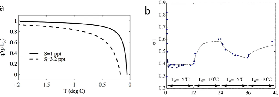
Fig. 5. (a) Energy of meltingqrelative to the latent heat of fusionρL0of pure ice, as a function of temperature for two values of salinity (Bitz
and Lipscomb, 1999, used with permission, American Geophysical Union). (b) Comparison of model predicted (solid line) and measured (dots) evolution of the mean solid volume fractionφ, for an experiment in which a 34 ppt NaCl solution is cooled from below with a varying temperatureT0(Notz and Worster, 2006, reprinted from Ann. Glaciol. with permission of the International Glaciological Society).
melting within brine inclusions. MU71 used a steady-state salinity profile computed from a series of Arctic multiyear ice cores (Schwarzacher, 1959). In addition, the latent heat of fusion was reduced at the lower boundary on the grounds that newly formed ice retains a liquid brine volume of about 10 %. Because of different values for the latent heat of fu-sion at the ice surface and at the ice base, the MU71 model is not energy-conserving and is not usable as it is in climate simulations. The mushy layer equations reduce to the MU71 model (Feltham et al., 2006) under several assumptions: ice and brine have the same density; brine flow and molecular salt diffusion in brine are neglected; ice salinity is constant in time; and only variations in the vertical are considered.
The MU71 model was the basis of the first sea ice com-ponent developed for large-scale climate models by Semtner (1976). Semtner did not keep MU71’s representation of the vertical salinity profile because the difference in latent heat of fusion between the upper and lower boundaries implies a violation of energy conservation. Instead, he proposed a simple formulation for penetrating radiation and brine vol-ume that conserves energy. During snow-free periods, the fraction of surface-penetrating radiation is stored in a heat reservoir, which represents internal meltwater. Energy from this reservoir is used to keep the temperature near the top of the ice from dropping below the freezing point, thereby sim-ulating release of heat through refreezing of the internal brine pockets.
The next generation of thermodynamic sea ice models was introduced by Bitz and Lipscomb (1999) (hereafter BL99). The BL99 model is based on MU71 but solves the problem of energy conservation when thermal properties depend on salinity and temperature by using the energy of melting (Un-tersteiner, 1961), i.e., the energy required to melt a volume of sea ice. The energy of melting is smaller than the latent heat
because it accounts for the presence of liquid brine, which reduces the energy that is required for full melting (Fig. 5a). In the original BL99 model, the vertical salinity profile is also Schwarzacher’s multiyear ice profile, variable in space but constant in time. The BL99 model and its derivatives (Winton, 2000; Vancoppenolle et al., 2007) constitute the ref-erence thermodynamic component of several large-scale sea ice models (Vancoppenolle et al., 2009b; Hunke, 2010).
In modeling the evolution of melt ponds, Taylor and Feltham (2004) explicitly used the mushy layer equations for heat transfer with the appropriate mixing equations for the heat capacity and the thermal conductivity (Eq. 4). They also kept a steady-state, vertically constant, 3.2 ppt salinity for the ice, since they were only interested in summer conditions.
A first attempt to couple the thermal effects of brine with ice desalination was made by Ebert and Curry (1993), who use the heat capacity and thermal conductivity parameteri-zations of MU71 but with a time dependence for ice salinity. For ice thinner than 60 cm they use the approximation of Cox and Weeks (1974), while a constant salinity of 3.2 ppt is used for thicker ice.
Notz and Worster (2006) introduced a fixed-grid enthalpy method which includes both mush and fully liquid regions within its domain, rather than the more traditional front tracking methods used in sea ice models. The model cor-rectly accounts for the redistribution of brine within the ice caused by brine expulsion and includes a model of flushing, where melt water at the surface flows through the ice accord-ing to Darcy’s law for flow in a porous medium. All the salt in the sea water is incorporated into the growing ice as found observationally in Notz (2005). Since this model is directly based on mushy layer theory, it realistically represents the impact of brine on sea-ice thermodynamics (Fig. 5b). How-ever, before the model can be used for climate studies, it needs to be extended to represent gravity drainage, a subject of ongoing work (Griewank and Notz, personal communica-tion).
Vancoppenolle et al. (2007) implemented the gravity drainage parameterization of Cox and Weeks (1988) into the BL99 model. The concept of an effective distribution coef-ficient (Sect. 2.2.1) is extremely helpful for the parameteri-zation of salt loss from sea ice. Mushy layer theory shows that brine fluxes from sea ice depend primarily on the buoy-ancy of the brine within the ice and on the permeability of the surrounding solid ice matrix. Hence, it would be desir-able to derive a formulation for a segregation coefficient that depends on these parameters, rather than on the ice growth rate. Such a physically based effective distribution coeffi-cient could then allow us to explain why, under certain ice-growth conditions, the very simplified and unphysical for-mulation ofkeffas derived by Burton et al. (1953) has proven to be quite successful in reproducing observed desalination rates (e.g. Cox and Weeks, 1988).
Nevertheless, Vancoppenolle et al. identified deficien-cies in the formulation of Cox and Weeks (1988) for gravity drainage: for example, the latter overestimates winter desali-nation in the lower half of the ice. Moreover, the empirical Cox and Weeks (1988) parameterization cannot be general-ized to the computation of biogeochemical tracers. In Van-coppenolle et al. (2010) and Jeffery et al. (2011), more realis-tic, diffusive formulations for gravity drainage are proposed. Vancoppenolle et al. (2010) represent gravity drainage using a turbulent diffusivity that is empirically enhanced when the depth-varying Rayleigh number (Notz and Worster, 2009) is super-critical. The results show substantial improvement compared to Cox and Weeks (1988). In contrast, Jeffery et al. (2011) propose a novel approach to modeling gravity drainage in one dimension by treating it as a diffusive pro-cess, using a diffusivity derived from mixing length theory.
Their model successfully reproduces the laboratory desali-nation sequence of Cottier et al. (1999) and the salt fluxes of Wakatsuchi and Ono (1983).
Vancoppenolle et al. (2007) also added a formulation for flushing, based on the following. Once the brine network is permeable over the entire sea ice layer, a fraction (30 %) of the melt water volume percolates through the brine network and replaces salty brine. The value of 30 % reflects the un-resolved three-dimensional features of the flow. Their model compares relatively well to observations of summer landfast sea ice desalination at Point Barrow (Fig. 6a). The simu-lated summer desalination is sensitive to parameters associ-ated with radiative transfer and fluid transport in the model.
A key question is how multiphase physics affects the sea ice mass balance. Vancoppenolle et al. (2005) have shown that the equilibrium thickness and ice-ocean salt fluxes in the BL99 model are quite sensitive to the representation of the ice salinity profile. The equilibrium thickness of about 3 m increases by up to one meter with salinity changes from 0 to 6 ppt for a vertically constant profile; higher ice salinity in-creases brine volume and specific heat capacity by up to two orders of magnitude. The increase in thermal inertia for more saline ice dominates the reduction in the energy of melting. Hence more saline ice resists warming more efficiently than fresh ice during the melt period, which in turn delays surface melt onset and reduces summer melt in the model used by Vancoppenolle et al. (2005). The shape of the profile was also found to be important, since low surface salinity is nec-essary to produce enough surface melt.
In a later study, Vancoppenolle et al. (2006) explored how temporal changes in the salinity profile affect the sea ice mass balance using the Vancoppenolle et al. (2007) model (Fig. 6b). The impact of salinity variations on ice thickness is concentrated during two key periods. First, during the sea ice growth period, high salinities found near the ice-ocean in-terface facilitate sea ice formation and reduce salt rejection. During the melt period, the decrease in ice salinity near the surface reduces thermal inertia and facilitates surface melt in the model.
3.1.4 Moving forward
m
ppt
kg/m
2
kg/m
2
m
year
month
no
rmalized
depth
mmol/m3
a
b
c
m
ppt
kg/m
2
kg/m
2
m
year
month
no
rmalized
depth
mmol/m3
a
b
c
m
ppt
kg/m
2
kg/m
2
m
year
month
no
rmalized
depth
mmol/m3
a
b
c
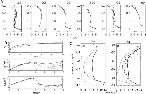
Fig. 6. (a) Vertical profiles of observed (stars) and simulated (lines) salinity during the early melt period of 2001 (day of year indicated at
the top of the panels), in the Chukchi Sea near Point Barrow (Vancoppenolle et al., 2007). (b) (top) 50-year time series of annual mean ice thickness in simulations using prognostic (solid line), steady-state isosaline (dash-dotted line), and steady-state, vertically-varying (dash-3x dotted line) salinity profiles. Time-integrated, seasonal cycle of total salt flux from the ice to the ocean for (middle) first-year and (bottom) 10-year-old multiyear ice. The lower panels also show salt flux from brine drainage (dotted) and equivalent salt flux from freshwater storage in the ice (dashed) for the prognostic salinity simulation (Vancoppenolle et al., 2006). (c) Normalized vertical profiles of the ice concentration of dissolved silicates in (left) June and (right) September for runs with (gray) and without (black) algal uptake associated with primary production. For comparison, field observations are also shown for sites in the Weddell Sea (pluses) and Bellingshausen Sea (diamonds). Panels (a) and (b) used with permission, American Geophysical Union. Panel (c) reprinted from Vancoppenolle et al. (2010) with permission from Elsevier.
gravity drainage based on the mushy layer Rayleigh-number, allow development of physically realistic and numerically ef-ficient schemes that can be used within large-scale models.
For both these approaches, modelers have to choose which combination of state variables they prefer to use. The most fundamental combination of state variables is arguably the enthalpy and the mass of salt contained within a model grid box. From these two fundamental variables, the tempera-ture, bulk salinity and solid fraction can uniquely be deter-mined. Given the equivalency between the state variables, a numerical scheme could also be based on the temperature and the bulk salinity within a grid cell. In its simplest for-mulation this latter choice requires an iterative cycle on the heat and solute equations to determine a liquid fraction (e.g. Petrich, 2005), while the choice of enthalpy necessitates a root finding method to convert between enthalpy and temper-ature, required for the conduction term in the heat equation
(e.g. Oldenburg and Spera, 1991; Notz, 2005). Independent of the choice of state variables, the resulting model allows one to simulate the evolution of the interior structure of sea ice based on first principles.
m
Fig. 7. The difference in sea ice thickness for a simulation em-ploying prognostic salinity relative to a simulation with the steady-state salinity profile of Schwarzacher (1959). (Vancoppenolle et al., 2009a, used with permission, American Geophysical Union.)
3.2 Numerical applications of multiphase physics
3.2.1 Climate modeling
Studies using large-scale sea ice models with various repre-sentations of multiphase physics point to the importance of (i) storage of latent heat within brine inclusions associated with the penetration of solar radiation into sea ice, (ii) the re-duction of the energy required to form or melt ice associated with significant liquid fractions, and (iii) the role of salinity on ice-ocean salt and freshwater exchanges.
In particular, MU71 found that brine inclusions retard the heating or cooling of the ice, and they argued that uncertain-ties in the salinity profile contribute to uncertainuncertain-ties in ice thickness. Likewise, using the zero-layer model of Semt-ner (1976) in a large-scale framework, SemtSemt-ner (1984) con-cluded that significant errors in phase and amplitude oc-cur if one neglects heat storage in thermodynamic sea-ice models. As a result, climate simulations using such ex-tremely simplified models have substantial biases that skew the seasonal disappearance of sea ice due to premature on-set of melt and increased melt rates. Similarly, Fichefet and Morales Maqueda (1997) showed that brine inclusions are the main contributor to the total heat content of Arctic sea ice. Nevertheless, Semtner’s zero-layer model and its derivatives are still the thermodynamic component of numerous large-scale sea ice models (e.g. Washington et al., 2000; Marsland et al., 2003; Timmermann et al., 2009; Hewitt et al., 2011).
The multilayer parameterization of sea ice desalination by Vancoppenolle et al. (2007) has been simplified further for inclusion in a large-scale, global, dynamic-thermodynamic sea ice model (Vancoppenolle et al., 2009b). Compared to a compilation of ice core salinity data, the simulated sea ice salinity shows spatial and temporal variations that are consis-tent with observations (Vancoppenolle et al., 2009a). First, the model agrees with observations in that the younger the ice, the more saline it is. In addition, Antarctic sea ice has a higher salinity than Arctic ice, in accordance with the saltier seawater, higher prevalence of young ice, and infiltration of snow by seawater. Furthermore, the sea ice salinity shows a seasonal cycle in both hemispheres, with higher values in winter and smaller values in summer.
Through a series of sensitivity simulations, Vancoppenolle et al. (2009a) studied the impact of ice salinity variations on sea ice. The order of magnitude of changes induced by salinity variations was found to be similar to a 10 % change in summer ice albedo, often presented as a key parameter. In the Arctic, salinity variations induce an increase in total ice volume by about 10 % via changes in the sea ice thermal properties, in particular the specific heat capacity and the en-ergy of melting (Fig. 7). In the Southern Hemisphere, the ice volume also increases. Ocean feedbacks amplify the differ-ences; with varying salinity, sea ice forms more efficiently while rejecting less salt into the ocean, which decreases ver-tical mixing and heat supply from the ocean to the ice.
The conclusions of all these studies underline the potential importance of sea ice salinity, but also stress the associated uncertainties and the need for more realistic representations of multiphase sea ice physics. In addition, our understanding of the impact of multiphase physics at large scales depends on the model used, at this stage the BL99 model, which ne-glects several aspects of sea ice multiphase physics. How-ever, it is interesting to note that more complex models have rarely contradicted the findings of earlier, simpler models. 3.2.2 Sea ice biogeochemistry
Development of sea ice biogeochemical models is less ad-vanced than that of sea ice physical models. In particular, multiphase physics and its coupling with nutrient, organic matter, trace metals and gases have been neglected or repre-sented in very simple terms. There could be nonlinear inter-actions between brine dynamics and biogeochemical sources and sinks (Vancoppenolle et al., 2010) such that biogeochem-ical impurities may behave differently from salt. For in-stance, fluid advection may fail to dislodge algae and some of the exudates, and thus nutrients incorporated into the al-gal biomass may accumulate in sea ice (Krembs et al., 2002; Raymond et al., 2009; Becquevort et al., 2009).
the required nutrients to sustain biological growth in the ice (Reeburgh, 1984; Fritsen et al., 1994). Convection is ei-ther confined in the lowermost, porous sea ice or may de-velop over the full depth of the ice, with a potential influ-ence on the localization of the communities. Second, dis-solved macronutrient concentrations in the ice plotted versus ice salinity lie on a line, in other words, the vertical profiles have the same shape, except when ice microbial communities are active, as indicated by field and laboratory experiments (Clarke and Ackley, 1984; Cota et al., 1987; Meese, 1989; Giannelli et al., 2001; Tison et al., 2008).
In principle, a model of sea ice biogeochemistry with a strong physical basis must represent how ice growth, melt and internal fluid transport affect the distribution of other in-clusions within the ice such as algae, nutrients, trace metals, and gases. Early sea ice biogeochemistry models handled the bio-physical coupling in various ways. Arrigo et al. (1993) represent the ocean-to-ice nutrient flux as the product of the nutrient concentration in seawater and a brine volume flux. This brine volume flux is formulated empirically, as a func-tion of the sea ice growth rate, based on the laboratory data of Wakatsuchi and Ono (1983). This approach was used later by Jin et al. (2006). Fritsen et al. (1998) included the con-tribution of flooding by seawater near the surface. In other studies, the nutrient fluxes were prescribed diffusivity values (e.g. Lavoie et al., 2005; Nishi and Tabeta, 2008). More re-cently, Tedesco et al. (2010) computed the fluxes of algae and nutrients from the ocean to the ice as directly proportional to the sea ice growth and melt rates. In all these studies, the fluxes of dissolved material missed some physical aspects of fluid transport.
Recently, the transport of solutes (e.g., nitrate, silicate, ammonium) has been included in one-dimensional sea ice models, based on transport equations containing some of the mushy layer physics (Vancoppenolle et al., 2010; Jeffery et al., 2011). In both studies, ocean and sea ice exchange dis-solved material in several ways. First, as for salt, disdis-solved tracers are trapped in the ice due to congelation at the ice base and due to flooding of snow by seawater at the ice sur-face. Second, dissolved tracers are redistributed within the ice due to gravity drainage and flushing. Finally, dissolved tracers are released in the ocean due to brine drainage and sea ice melt. Vancoppenolle et al. (2010) combined their pas-sive tracer module with a prescribed uptake due to primary production in sea ice, in order to simulate the vertical profile of dissolved silicates in Antarctic sea ice (Fig. 6c). The re-sults give qualitative agreement of the silicate profiles with observations. Jeffery et al. (2011) validated their formula-tion using brine salinity as a tracer, and conclude that theirs is a viable choice for simulating biogeochemical tracers in sea ice.
Sea ice modelers have not begun to incorporate the vapor phase, although it may play a significant role in gas transfers between ocean and atmosphere with potentially significant consequences for atmospheric chemistry and climate (Loose
et al., 2011). For instance, methane venting has been ob-served under sea ice at high latitudes (e.g., Shakhova et al., 2010), and sea ice halogen chemistry is critical for ozone depletion in the polar atmospheric boundary layer (Simpson et al., 2007).
There are many open questions regarding brine-biogeochemistry coupling in sea ice. What is the impact of the representation of multiphase physics on sea ice biogeochemistry? Are there several modes of transport of sea ice impurities (active, passive transport) that should be taken into account? Moreover, bio-physical feedbacks may impact larger scale, physical sea ice and climate processes (e.g., Lengaigne et al., 2009); the importance of biogeo-chemical processes for climate has yet to be ascertained. These questions need to be addressed via modeling and experimental studies.
4 Observations
Any progress in our theoretical understanding or numerical simulation of the multiphase physics of sea ice must be eval-uated against reality. However, detailed measurements of the temporal and spatial evolution of sea-ice microstructure are still largely lacking, despite progress in recent years. For ex-ample, the vertical profile of brine velocity is critical to the evolution of the salinity profile and tightly coupled with the permeability of the ice, but challenging to measure. In this section we briefly summarize the most relevant measurement techniques and point out particular data needs that will hope-fully be addressed by sea-ice researchers in the near future.
Traditionally, ice-core measurements have been the stan-dard approach to gain insight into the internal structure of sea ice. For such measurements, an ice core is extracted from an ice floe and then usually cut into thin slices. These are often examined visually to obtain their crystal structure and brine-channel distribution, for example. More objective analysis of the microstructure of such samples has recently become possible by direct three-dimensional imaging using conven-tional X-ray tomography (Golden et al., 2007; Pringle et al., 2009b) or the more highly resolved synchrotron-based X-ray microtomography (Maus et al., 2010a,b). Melting the ice-core samples allows one to measure bulk salinity profiles, to analyze the isotopic composition and hence the amount of meteoric water content (e.g. Eicken et al., 2002), or to obtain the algal biomass, nutrients and trace metals (Arrigo et al., 2010, and references therein). Additional information on the gas content of the ice can be gained by measuring the den-sity of the samples (Cox and Weeks, 1983) or by direct gas extraction (Nakawo, 1983; Tison et al., 2002; Rysgaard and Glud, 2004; Tison et al., 2010; Stefels et al., 2011), which has recently received much attention with respect to the role of sea ice in the Arctic CO2budget.
(e.g., Weyprecht (1879) and Malmgren (1927)), the overall data set remains too sparse to reliably test numerical models that describe the multiphase physics of sea ice. For example, we still have only very few data sets that allow for the anal-ysis of the temporal evolution of sea ice salinity, crucial to reliably test numerical predictions. Among the most notable ice core studies in this respect are the data set by Nakawo and Sinha (1981) who took bi-weekly sea-ice samples through-out a whole winter season; the data set provided by the Uni-versity of Alaska, Fairbanks of cores taken north of Alaska (Eicken, 2011); and a data set of Antarctic ice cores (Aus-tralian Antarctic Data Center, 2011). The apparent lack of temporally and spatially resolved data from ice core studies is caused by two main difficulties. First, ice-core extraction and analysis cannot easily be automated, which is why both spatial and temporal resolution of most ice-core studies are too low to reliably relate their results to numerical simula-tions. Second, ice-core studies are necessarily destructive and it is impossible to track temporal evolution of sea-ice microstructure within the same sample.
In addition to these difficulties, all such studies suffer from the fact that usually some brine is lost from the core during its extraction. This leads to particularly large sampling errors within the biologically important, porous bottom layer of the ice sample (e.g., Notz et al., 2005). While methods have been developed to minimize the loss of brine during sampling of sea ice (Cottier et al., 1999), these are usually difficult to ap-ply in the field. Therefore, focus has recently turned to non-destructive methods that allow for in-situ sampling of sea-ice properties. Regarding the multiphase structure of sea sea-ice, these methods include measurements of complex permittiv-ity with capacitance probes (Morey et al., 1984; Backstrom and Eicken, 2006; Pringle et al., 2009a), cross-borehole re-sistivity tomography (Ingham et al., 2008) and parallel-wire impedance measurements (Notz et al., 2005), which have all been summarized in more detail by Pringle and Ingham (2009). These methods pose some potential to overcome the limitations of classical ice-core studies, most notably be-cause they allow for the automated measurement of the tem-poral evolution of the solid and the brine fractions of sea ice. Further development of these methods and their wider ap-plication in both field and laboratory studies will allow for an increased understanding of desalination processes as well as the small-scale horizontal variability of sea-ice microstruc-ture. Measurements are required that cover the full cycle of sea-ice formation in open water, its growth during winter, the impact of flushing with surface melting during summer and the eventual decay of the ice cover. For the modeling of Antarctic sea ice, data sets are also needed regarding sea ice flooding caused by a heavy snow pack, in particular regard-ing the incorporation of this water into the ice pack and its impact on the internal structure of the ice.
In addition to such automated measurements of sea-ice mi-crostructure, we also require far more data regarding the tem-poral evolution of the biologically and climatically
impor-tant gas content of sea ice. So far, there exist very few data sets of its temporal evolution, many of which focus on the CO2 exchange at the ice-atmosphere interface using either eddy correlation techniques (Baldocchi et al., 1988; Oechel et al., 1998) or chamber techniques (Livingston and Hutchin-son (1995) and references therein; see also Schrier-Uijl et al. (2010) and Loose et al. (2011)). This lack of data is due, to some degree, to the fact that sea ice has for a long time been regarded as an impermeable lid on the ocean (Tison et al., 2002; Bates and Mathis, 2009), despite early works that clearly demonstrated significant gas exchange through sea ice (Gosink et al., 1976). Therefore the contribution of sea ice to gas exchange has only relatively recently be-come a major focus of polar research (Semiletov et al., 2004), leading to a significant increase in measurement campaigns (e.g. Delille et al., 2007; Rysgaard et al., 2009; Papakyriakou and Miller, 2011). However, more measurements clearly are needed to support development of realistic biogeochemistry components in large-scale, coupled numerical models.
The same holds for data regarding the interaction of sea ice with its snow pack (Sturm and Massom (2010) and refer-ences therein). Even a thin layer of snow significantly alters the heat budget of the ice because the thermal conductivity of snow is much lower than that of sea ice, and because snow often has a much larger albedo than bare ice. Melting snow that percolates into the ice leads to flushing and hence low-ers sea-ice salinity, but it can also create impermeable laylow-ers within the ice that foster the formation of surface melt ponds (Eicken et al., 2002; Vancoppenolle et al., 2007). Despite the importance of snow on sea ice, there are very few de-tailed measurements of its characteristics and fewer measure-ments of their temporal evolution. Here, again, more data are needed to allow for a better representation of the interaction of snow with sea-ice microstructure in numerical models.
While the clear data requirements described in this section are mostly motivated by the evaluation of numerical mod-els, the same data is also essential for evaluating or using satellite products. For example, reliable salinity measure-ments are needed for algorithms for deriving sea-ice thick-ness from measurements by ESA’s “Soil Moisture and Ocean Salinity (SMOS)” satellite (Kaleschke et al., 2010), whereas improved data sets of sea-ice microstructure and of sea-ice density are crucial to better estimate sea-ice thickness esti-mates that are based on freeboard measurements from space (ICESAT, CRYOSAT). The success of these satellite mis-sions crucially depends on the existence of a large data pool of reliable in-situ measurements.
5 Conclusions
the basic premise that a salinity profile representative of mul-tiyear ice was sufficient for modeling sea ice. While physi-cal processes have garnered most of the attention paid to the role of sea ice in the polar climate system, it has become in-creasingly obvious that chemical and biological changes are important to fully understand that role. This is the more the case with the ongoing transition of the Arctic from a multi-year sea-ice pack to one with a high percentage of first-multi-year ice. Thus, changes in the physical system along with the progression of modeling capabilities into the biogeochemi-cal domain have renewed scientific interest in sea ice halo-dynamics and multiphase physics.
Observations, both in the field and in the laboratory set-ting, have revealed the complex structure of sea ice and the dynamic processes that result from and cause that structure. Field research has further uncovered the subtle and often sur-prising role of sea ice multiphase physics in polar chemical-and ecosystems, as a concentrator of nutrients, incubator of algal life, and pathway for gas exchange between ocean and atmosphere. Experimental campaigns are beginning to fill the large gaps in data describing sea ice multiphase physics, but much more data is needed to fully understand the mecha-nisms and their dependencies, time evolution and variability. While climate modelers forge ahead with the model-ing frameworks at hand, new theoretical and numerical ap-proaches are being developed based on the extensive body of knowledge already compiled in metallurgical multiphase applications. For example, mushy layer theory (borrowed from solidification physics) provides a useful description of the general properties of sea ice by averaging over the mi-crostructure. The role of the five basic desalination processes (initial salt rejection, brine diffusion, brine expulsion, grav-ity drainage and flushing) of sea ice has been explored and the importance of each process determined. As discussed in Sect. 3, models are being developed and implemented nu-merically that address the sea ice salinity problem at various scales ranging from the microstructure to global, in one, two and (perhaps) three dimensions. A standardized model in-tercomparison of a small set of common problems could be useful for translating the highly resolved physical processes into parameterizations feasible for use in GCMs.
Recent modeling studies that include large-scale represen-tations of complex sea ice multiphase physics highlight the importance of such parameterizations for accurate simula-tions of polar climate. Furthermore, modelers are now be-ginning to examine the effect of sea ice’s microstructure and salinity evolution on organisms living in the ice, a subject long debated only in observational circles. Sea ice multi-phase physics is a very vibrant field of research that brings together observationalists, theorists and numerical modelers, all with the goal of improving our understanding of earth sys-tem changes, both polar and global, and the role of sea ice in these changes.
Acknowledgements. We thank Hajo Eicken for suggesting this
review and for enlightening discussions on the topic. Scott Elliott kindly read and commented on the manuscript also, for which we are grateful. We further thank S. Ackley and an anonymous reviewer for their careful reading and constructive comments. Hunke and Turner acknowledge funding from the Biological and Environmental Research division of the U.S. Department of Energy (DOE) Office of Science; Los Alamos National Laboratory is operated by the National Nuclear Security Administration of the DOE under Contract No. DE-AC52-06NA25396. Vancoppenolle is funded by Belgian FNRS, and Notz acknowledges funding through the Max-Planck-Society. This review paper resulted from the workshop “The Multi-Phase Physics of Sea Ice: Growth, Desalination and Transport Processes” held 8–10 September 2010 in Santa Fe, New Mexico, and funded through the DOE Office of Science project “Improving the Characterization of Clouds, Aerosols and the Cryosphere in Climate Models.”
Edited by: J.-L. Tison
References
Ackley, S. F., Lewis, M., Fritsen, C., and Xie, H.: Internal melting in Antarctic sea ice: Development of “gap layers”, Geophys. Res. Lett., 35, L11503, doi:10.1029/2008GL033644, 2008.
Andreae, M. O. and Raemdronck, H.: Dimethyl sulfide in the sur-face ocean and the marine atmosphere: A global view, Science, 221, 744–747, 1983.
Andreas, E. L. and Ackley, S. F.: On the differences in ablation seasons of the Arctic and Antarctic sea ice, J. Atmos. Sci., 39, 440–447, 1982.
Arrigo, K., Worthen, D. L., Lizotte, M. P., Dixon, P., and Dieck-mann, G.: Primary production in Antarctic sea ice, Science, 276, 394–397, 1997.
Arrigo, K., Mock, T., and Lizotte, M.: Primary producers and sea ice, in: Sea Ice, edited by: Thomas, D. N. and Dieckmann, G. S., 283–326, Wiley-Blackwell, Oxford, UK, 2010.
Arrigo, K. R., Kremer, J. N., and Sullivan, C. W.: A simulated Antarctic fast ice ecosystem, J. Geophys. Res., 98, 6929–6946, 1993.
Assur, A.: Composition of sea ice and its tensile strength, in: Arc-tic sea ice; conference held at Easton, Maryland, February 24– 27, 1958, Vol. 598 of Publs. Natl. Res. Coun. Wash./, 106–138, Washington, DC, US, 1958.
Australian Antarctic Data Center: Sea Ice Measurements Database, http://data.aad.gov.au/aadc/seaice/, online; last access: 21 March 2011, 2011.
Backstrom, L. G. E. and Eicken, H.: Capacitance probe measurements of brine volume and bulk salinity in first-year sea ice, Cold Reg. Sci. Tech., 46, 167–180, doi:10.1016/j.coldregions.2006.08.018, 2006.
Baldocchi, D. D., Hincks, B. B., and Meyers, T. P.: Measuring biosphere-atmosphere exchanges of biologically related gases with micrometeorological methods, Ecology, 69, 1331–1340, 1988.