Max Planck Institute for Demographic Research Konrad-Zuse Str. 1, D-18057 Rostock·GERMANY www.demographic-research.org
DEMOGRAPHIC RESEARCH
VOLUME 26, ARTICLE 22, PAGES 593-632
PUBLISHED 13 JUNE 2012
http://www.demographic-research.org/Volumes/Vol26/22/ DOI: 10.4054/DemRes.2012.26.22
Research Article
Point process models for household distributions
within small areal units
Zack W. Almquist
Carter T. Butts
This publication is part of the Special Collection on “Spatial Demography”, organized by Guest Editor Stephen A. Matthews.
c
⃝2012 Zack W. Almquist & Carter T. Butts.
2 Human settlement patterns 595
3 Background on spatial data and household distributions 596
3.1 Spatial data 597
3.2 Household distributions 598
4 Point process models and simulation 598
4.1 Constant-intensityN-conditioned Poisson process model (uniform) 599 4.2 Low-discrepancy sequence model (quasi-random) 600 4.3 Inhomogeneous Poisson process model (attraction) 600
4.4 Point stacking and building heights 601
5 Standard statistical measures for point processes 601
5.1 Ripley’sKfunction 601
5.2 Nearest neighbor measures 602
5.3 Scan statistics and baseline models 603
6 Comparison data: U.S. Census geography and household parcel lots 603
6.1 U.S. Census geography 603
6.2 Household distribution data in the US 604
6.3 Urban, suburban, and rural classification 604
7 Comparison measure 611
8 Analysis and results 612
8.1 Software 612
8.2 Comparison of point distributions 612
9 Example: Network diffusion over a spatially embedded network 617
9.1 Spatial Bernoulli Graphs and Simulation 621
9.2 Network diffusion 622
9.3 Simulated diffusion over Portland, OR 623
10 Conclusion and discussion 625
11 Acknowledgments 626
Point process models for household distributions
within small areal units
Zack W. Almquist1
Carter T. Butts1,2
Abstract
Spatio-demographic data sets are increasingly available worldwide, permitting ever more realistic modeling and analysis of social processes ranging from mobility to disease trans-mission. The information provided by these data sets is typically aggregated by areal unit, for reasons of both privacy and administrative cost. Unfortunately, such aggregation does not permit fine-grained assessment of geography at the level of individual households. In this paper, we propose to partially address this problem via the development of point pro-cess models that can be used to effectively simulate the location of individual households within small areal units.
1.
Introduction
Spatio-demographic data sets are increasingly available worldwide, permitting ever more realistic modeling and analysis of social processes ranging from mobility to disease trans-mission. The information provided by these data sets is typically aggregated by areal unit (e.g., the state, county, tract, block group, and block hierarchy of the U.S. Census), for reasons of both privacy and administrative cost. Unfortunately, such aggregation does not permit fine-grained assessment of geography at the level of individual households, a scale that is potentially important for accurate modeling of micro-social processes such as transmission of disease between households, daily mobility patterns, or patterns of inter-personal contact. While the potential to model such phenomena across large geographical areas thus exists, efforts are hampered by a lack of data on household location.
In this paper, we propose to partially address this problem via the development of point process models that can be used to effectively simulate the location of individual households within small areal units. Given basic information such as number of house-holds, general pattern of land use, and/or population of neighboring units, our objective is to identify a probability distribution over household locations within a polygonal re-gion whose average spatial properties reflect the corresponding properties of the unob-served true household distribution in that region. Examples of targeted properties include standard point process descriptives (Ripley 1988; Diggle 2003), such the mean nearest neighbor distance, measures of spatial clustering (e.g. theF andGfunctions), meanK function value, et cetera. While the resulting distributions will not reproduce household locations with perfect fidelity, the approximations may nevertheless prove adequate for modeling of basic social processes. The models and test procedures proposed in this re-search also provide relatively generic techniques for statistical treatment of other forms of geocoded point data localized only to an areal unit (e.g., locations of individuals, events, or landmarks).
house-hold location data from Portland, OR, Deschutes County, OR, and Irvine, CA2, with areal
units given by the 2000 U.S. Census. All modeling is performed inR(R Development Core Team 2010). Our test cases include examples of urban, suburban, and rural settings, with varying spatial scale and levels of population density.
Evaluation of the suggested point processes on our three communities suggest that simple models can provide quite reasonable approximations of household location distri-butions for small areal units. Performance degrades substantially for larger units, although the inhomogeneous model shows some potential within more urbanized regions. Practical suggestions are given for the use of these and related point processes within large-scale simulations, and for applications of this technique to settings beyond the U.S. (and the developed world more generally).
The remainder of the paper is organized as follows: (1) a general discussion of human settlement patterns; (2) background on spatial data and household distribution; (3) an introduction to the proposed point process models; (4) standard statistical measures for point processes to be used for evaluative purposes; (5) comparison data and U.S. Census geography to be used for our evaluation study; (6) the comparison measures used for our evaluation study; (7) evaluation study analysis and results; (8) a spatially informed network diffusion example; and, finally, (9) conclusion and discussion.
2.
Human settlement patterns
Settlement patterns play an important role in shaping human interaction and the demo-graphic processes which result. A classic example is that of marriage in modern Western societies: couples in such societies rarely marry without prior meeting and extensive face-to-face interaction, and marriage is thus disproportionately propinquitous (Bossard 1932). Many demographic processes, such as mortality, fertility, and mobility, are also influenced by human settlement patterns (see, e.g. Freeman and Sunshine 1976; Guilmoto and Ra-jan 2001; Binka, Indome, and Smith 1998); however, making use of such geographical information is frequently difficult due to limitations on data availability. For example, in the United States information on population within aggregate areal units is readily avail-able (e.g., via the U.S. Census), but the coordinates of individuals and households are undisclosed due to privacy concerns. There is thus a distinct need for a methodology to generate household (or individual) distributions over small scale areal units such as census geography, so as to inform statistical models, agent-based simulations, and the like.
Adding to the difficulty of this problem is the need for plausible models to be easily computable. For instance, the year 2000 U.S. census reports population in over 8 million
areal units known asblocks, themselves organized into well over 50,000tracts(US Cen-sus Bureau 2001). Applying household location models at national or regional scales thus requires simulation of location distributions for large numbers areal units, making effi-ciency an important concern. In addition to computability, models to be used in a range of settings should be simple, robust, and require minimal information input on the part of the analyst. (For instance, a household location model requiring detailed street maps may be of limited use in historical applications, or in countries for which such maps are not readily available.) Such concerns motivate the initial consideration of highly mini-mal models that employ as little information as possible and that can be easily simulated for large numbers of areal units. Following Mayhew (1984a), we regardbaseline models
(and minor extensions thereof) as a natural starting point. By beginning with basic, read-ily available information such as counts of households and areal unit boundaries, we first construct models that treat household placement as conditionally uniform, subsequently modifying this assumption by introducing higher “evenness” in placement, and then by allowing household location probability to be affected by the geometry of the areal unit in which it resides. To the extent that the resulting models produce household distributions whose properties approximate those observed in real settings, we regard them as adequate proxies with respect to those properties. Where these simple models fail, they may nev-ertheless be used as a starting point for building more complex models (e.g., models with inter-point interaction, or additional covariates) for particular applications.
3.
Background on spatial data and household distributions
a polygonal region (including artificial elevation) whose average spatial properties reflect the corresponding properties of the unobserved true household distribution in that region.
3.1 Spatial data
Spatial information associated with spatio-demographic data includes, but is not limited to, points (single locations, e.g., a house), lines (e.g., a road), and polygons or areal units (e.g., a Census block). Typically, Geographic Information Systems (GIS) are employed for handling and performing analysis on a myriad of spatial data (Reibel 2007); in par-ticular, this includes linking spatial coordinates to socio-economic and demographic data. For the present problem, the two most important spatial units are those of the point and the polygon. A point consists ofX andY coordinates (e.g., longitude and latitude, or a pro-jection thereof into the plane) and a polygon represents a series of line segments (again in either latitude/longitude or planar coordinates) identifying a closed region on the Earth’s surface. Because of the curvature of the Earth’s surface, most map-based and related cal-culations are based on points and polygons that have beenprojected onto a plane; the choice of map projection can have non-trivial effects for such important measures as in-terpoint distances and polygonal areas, and thus must be chosen carefully. Fortunately, when working with small areal units such as those employed in this paper, distortions due to projection are easily overcome (e.g., by using orthonormal projections about the centroid of the areal unit). More details on choice of projection and coordinate system can be found in Snyder (1987).
The process of attaching or associatinggeographic coordinatesto attributes (e.g., lo-cations of houses, cars, or individuals) is known asgeocoding. New developments in online data processing and management have allowed for larger-scale and higher quality geographic data collection by both professionals and nonprofessionals than was possible in previous decades. The geographic literature refers to nonprofessional geocoding as
3.2 Household distributions
There exists a plethora of reasons to be interested in the distribution of human popula-tions over space, and particularly the location distribution of human households. Humans have since prehistory gathered together in small groups (often kin groups) to manage their livelihoods (McC. Netting, Wilk, and Arnould 1984), and we loosely refer to a group of persons residing at the same location and sharing resources as ahousehold. In the mod-ern context, households are often studied as units of decision making (e.g., Davis 1976), criminological and neighborhood processes (e.g., Hipp, Faris, and Boessen 2012; Short et al. 2010), disease and information spread (Salathé and Jones 2010), et cetera. Here, we focus on the household as our basic unit of interest. The study of household activities over spatially diverse contexts has been performed primarily through the concatenation of administrative data (e.g., censuses) and spatial data (e.g., surveys or sensors) to make var-ious predictions, forecasts and simulations for scientific and public policy reasons (Fox et al. 2003). It is common to use spatial data at a largely aggregate level (e.g., a U.S. census tract), and this has allowed for much scientific progress; however, reliance on ag-gregate data raises concerns regarding the risks of fallacious ecological inference (Gibson, Ostrom, and Ahn 2000) and the modifiable areal unit problem (Openshaw 1984; Tobler 1979; Martin and Bracken 1991). Another issue with aggregate data is that it does not allow for certain types of analysis necessary for social science, public health, or demo-graphic research. Here, we are particularly concerned with the situations in which one cannot conduct one’s analysis without household-level spatial information, such as mod-eling of transmission of disease between households, daily mobility patterns, or patterns of interpersonal contact. Because administrative and archival data often lacks individual or household locations, we propose in this research to use point process probability mod-els to simulate household distributions over administrative polygons which maintain key statistical properties of interest.
4.
Point process models and simulation
A point process is defined mathematically as a random element whose support consists ofpoint patternson a point setS. Technical considerations are needed to ensure that the resulting process is well-defined (see, e.g. Stoyan, Kendall, and Mecke 1987), but for our purposes it is sufficient to think of a point pattern as a countable subset ofS.
some fixed probability density function. More formally, ahomogeneous planar Poisson processmay be characterized by the following two conditions:
i) For someλ≥0, and any finite planar regionS,N(S)(the number of events with corresponding points inS) follows a Poisson distribution with meanλ|S|, where|S| is the area ofS. (Note that, here,λis called theintensityof the process.)
ii) GivenN(S) = n, thenevents inSform an independent random sample from the uniform distribution onS.
It is worth noting that λ|S|is the integral ofλoverS, and thus to specify an inho-mogeneous planar Poisson process, one need only replace the constantλby a spatially dependent intensityλ(x, y)—replacing condition (i) with “for someλ(x, y)≥0, and any finite planar regionS,N(S)follows a Poisson distribution with mean∫Sλ(x, y)dxdy” and modifying condition (ii) to specify that events are drawn independently proportional toλ(x, y)(rather then uniformly). Apart from certain basic regularity conditions (in par-ticular,λ(x, y)must have a finite integral over all subsets ofS), there are few restrictions regarding the intensity function; the inhomogeneous spatial Poisson process is thus a fairly flexible tool for representing location distributions.
The Poisson processes form only one of a wide range of point process classes that may be employed to simulate household location distributions. Here, we employ three variant processes, the first of which is an application of the uniform or homogeneous process (conditioned on region boundaries and observed population), the second of which is a deterministic low-discrepancy process that behaves much like a uniform distribution (but tends to place households away from one another), and the third of which is an inhomogeneous Poisson process whose intensity function (λ) depends on proximity to unit boundaries. We now consider each of these processes in turn.
4.1 Constant-intensityN-conditioned Poisson process model (uniform)
4.2 Low-discrepancy sequence model (quasi-random)
The low-discrepancy sequence model (henceforth referred to as theQuasi-randommodel) is a near-minimal entropy distribution in which households are placed in an extremely even, “grid-like" manner using a two-dimensional Halton sequence. A Halton sequence is a deterministic sequence of points that “fills” space in a uniform manner, while also main-taining a high nearest-neighbor distance. The result (sometimes called a “quasi-random” distribution) is similar to a set of draws from the uniform distribution, but substantially more evenly placed (see Gentle 1998, for algorithmic details). A sample realization of such a process may be seen in Figure 6(d).
4.3 Inhomogeneous Poisson process model (attraction)
The above homogeneous models treat households as equally likely to lie in any constant-area region within the target polygon; in fact, however, we have reason to suspect that households will often concentrate around certain features, a fact that may be exploited to better-approximate their distribution. The edge-attractive inhomogeneous Poisson pro-cess model (henceforth referred to as theAttractionmodel) is one in which we assume that points are distributed such that they cluster around polygon boundaries. This is con-trolled by a givenpoint potentialfunction defining the intensityλ(x, y). We consider two forms for the potential function, which are defined as follows. LetZbe a collection of line segments (indicating boundaries of the areal unit, internal polygons (such as subsidiary unit boundaries), or elements such as roads), and letd((x, y), z)forz ∈Zbe the mini-mum distance between the point(x, y)and the line segmentz. We then set the intensity to be
λ(x, y) = max
z∈Z
(
1 +d((x, y), z)−o
s
e), (1)
wheresis a scale factor, ois an “optimum” distance, andeis an exponent. For most applications, it is reasonable to select the parameterss, o,andesuch thats >0,o≥0, ande <0. Intuitively, the resulting point potential attracts points to polygon boundaries (or, more generally, the elements ofZ), with maximum intensity occurring when one is at distanceofrom a line segment. This definition is motivated by the frequent use of roads, waterways, or other similar physical elements as boundaries of areal units: housing units are often located along such features, but are frequently offset by some amount. For a sample realization of this process see Figure 6(b).
search to find values ofsandethat produced highest averagep-values over all aggregated cases in the test data (described below). This resulted in parameter values ofs= 0.00015
ande = −1.5 (with the former in angular units). Experimentation suggested that the results reported here are reasonably robust to these settings, and minor changes do not greatly change the resulting point patterns.
4.4 Point stacking and building heights
For all of the point process models used here, we also avoid unrealistic ground-level congestion by means of a simpleartificial elevation model, which simulates the effects of multi-story residential structures in densely populated blocks. Specifically, households whose ground position would place them within a 10m radius of k previously placed households are given a vertical elevation of 4kmeters; thus, intuitively, artificial elevation arises as population density grows, with new households “stacking” on old ones. (Arrival order is treated as random.) Building heights produced by this method appear generally consistent with the ranges of residential building heights typically reported in the literature (e.g., Burian, Brown, and Velugubantla, 2002). Finally, within-household proximity is maintained by requiring household size to satisfy the known marginals within each areal unit, and then placing individuals at their household locations (jittering randomly within a 5m radius to avoid exact overlap).
5.
Standard statistical measures for point processes
In order to compare the distribution of household locations arising under our models to those empirically observed, we require appropriate descriptive statistics. Here, we de-scribe several standard descriptives from the point process literature, that may be em-ployed to assess the extent to which simulated household distributions do or do not deviate from their empirical counterparts.
5.1 Ripley’sKfunction
5.1.1 TheoreticalK
TheKfunction is defined as:
K(s) = 1
λE[number of other events within distancesof a randomly chosen event], (2) whereλis the density (number per unit area) of events; thus,Kdescribes characteristics of a point process at different distance scales. Note that many alternative standard mea-sures such as the nearest neighbor methods (see Section 5.2) do not have this property.K is generally the preferred characterization of spatial point process by statisticians and ge-ographers (see, e.g. Diggle 2003), and we use it as the basis of our empirical investigation in Section 8.
5.2 Nearest neighbor measures
In addition to the variation in conditional density through space, one can also consider point processes in terms of their nearest-neighbor properties. Here, we comment on two functions of this sort that are of potential utility in assessing point pattern adequacy.
5.2.1 GFunction
The G function measures the distribution of the distances from an arbitrary event to the nearest other event (see, Diggle 2003). Usually these distances are denoteddi =
minj{dij∀j̸=i},i= 1, . . . , n, so that theGfunction is
G(r) =#{di : di≤ri, ∀i}
n , (3)
where the numerator is the number of elements in the set of distances that are lower than or equal tod, andnis the total number of points.
5.2.2 FFunction
TheFfunction measures the distribution of all distances from an arbitrary point of the plane to the nearest realized event (see, Diggle 2003). Bivand, Pebesma, and Gómez-Rubio (2008) notes that this function is often called theempty spacefunction because it is a measure of the average space left between events. (Note the contrast withG, in which the focal point is itself a realized event.) TheFfunction of a stationary point processX is the cumulative distribution functionFof the distance from a fixed point in space to the nearest point ofX. Under CSR,Fis:
5.3 Scan statistics and baseline models
Historically, much of the statistical literature on point process models has been concerned with locating clusters of interest (often the relevant descriptives are known asscan statis-ticsorKulldorff scan statistics). Sample applications include identification of clusters of trees, ant nests, diseases, or post offices (Costa and Kulldorff 2009). Classically, the aim of the spatial scan statistic is to detect and evaluate the statistical significance of a spa-tial cluster of events (broadly defined) that cannot be explained by Bernoulli or Poisson processes. Note that these models are often focused on an attribute associated with the points and not with the point distribution itself (unlike the present case). Models for scan statistics were originally proposed by Naus (1965) and have recently been extended by Kulldorff (1997) and others (Glaz, Pozdnyakov, and Wallenstein 2009). Although broadly related, it is worth pointing out that the goal of most research using scan statistics is very different from the goal of this research. We are interested in characterizing a set of points within a areal unit and demonstrating which distributions provide the best baseline model for simulation purposes. Note that one could use these same models and statistical tests for novel baseline models (as described in Mayhew 1984a) for explaining/exploring the processes behind geocoded data. Extension of the present problem into this arena would seem to be a promising avenue for further research.
6.
Comparison data: U.S. Census geography and household parcel
lots
To evaluate the above models, we seek to compare their resulting simulated household distributions with those encountered in realistic settings. Although household location data is difficult to obtain, we are able to employ parcel data from three U.S. communities for testing purposes. While not representative of all communities worldwide, we view these three cases as a “proof of concept” for the wider use of settlement pattern imputation from simulation models like those employed here.
6.1 U.S. Census geography
population aggregation. The block represents household or individuals aggregated at the level of city block (if the population density is sufficient not to jeopardize an individu-als privacy) or larger unit; block groups represent an aggregation of blocks, and tracts represent an aggregation of block groups (US Census Bureau 2001). This data is made available through the U.S. Census website3, and through statistical software such as the
UScensus2000 R-package (Almquist 2010).
6.2 Household distribution data in the US
There is limited access to household data in the United States, and this can be even more difficult in other countries. In some cases, however, household-level geospatial data may be acquired from cities and counties across the U.S. that is collected for purposes of local or state property tax administration. This household data available is known as
parcel data, and is either maintained as shapefiles or simple longitude/latitude point files; typically this data is difficult and time consuming to acquire when available.4To provide
an empirical comparison set for our point process models, we have acquired three different sets of parcel data within the US: an urban setting (Portland, OR), a suburban setting (Irvine, CA), and a rural setting (Deschutes County, OR). For an example see Figure 6(a). Although a more general, representative sample of parcel data is not available at this time, the range of urbanization in our three cases provides some suggestion of how model performance might vary across similar communities in the United States or other countries with comparable settlement patterns.
6.3 Urban, suburban, and rural classification
The U.S. Census classifies areas as eitherurbanorrural. Urban areas are broken into two classifications:Urbanized Areas (UA), continuously built-up areas with populations of 50,000 or more; and,Urban Places Outside of UAs, any incorporated places or census designated places (CDPs) with at least 25,000 inhabitants. The rural designation is defined residually, i.e. territory, population, and housing units that the Census Bureau does not classify as urban are classified as rural (US Census Bureau 2001).
We extend the U.S. Census Urban/Rural classification to include a notion ofsuburban. “Suburban areas are typically considered to be regions of lower density residential land use at the urban fringe, and are often thought to be synonymous with sprawl, but there is no standard quantitative definition" (Theobald 2004). The notion of Suburbia is old, being found in the sociological literature as far back as 1943 (Harris 1943). In this case we use
3http://www.uscensus.gov
the concept of suburb to represent a city which is less dense than an urban center, resides in or near a large metropolitan area, and that is not the focal city within the Metropolitan Statistical Area (MSA) itself (i.e., the largest city within the MSA, e.g., Los Angeles MSA; US Census Bureau 2001). Of our three cases, we treat Irvine, CA as suburban because it belongs to an MSA (but is not focal), is less dense than an urban center, and is distinctive for both historical and geographical reasons (i.e., it is a planned suburban city residing near the more clearly urban environments of Los Angeles and Santa Ana).
An alternative way to conceptualize this distinction is via housing density (or popu-lation density).5 The urban, suburban, rural classification here can be thought of as an average housing density scale with urban being high density, suburban being middle den-sity, and rural being low density (see Table 1). A quick inspection shows that the mean housing density is approximately double from the rural to suburban setting and also ap-proximately double from suburban to urban setting. And thus we may also think of these three examples as sitting on density continuum which we are labeling with discrete names.
Table 1: Table of mean housing densities per census areal unit for Portland,
OR, Irvine, CA, and Deschutes County, OR
Area Mean density
Urban Portland block 1.4195#houseskm2
Portland block group 1.1906#houseskm2
Portland tract 1.0641#houseskm2
Suburban Irvine block 0.7139#houseskm2
Irvine block group 0.5707#houseskm2
Irvine tract 0.3597#houseskm2
Rural Deschutes block 0.3615#houseskm2
Deschutes block group 0.2313#houseskm2
Deschutes tract 0.1599#houseskm2
With this classification in mind, we briefly consider our three cases in turn.
6.3.1 Urban: Portland, OR
Portland, Oregon is a city with an estimated population of 529,121 people and estimated household population of 223,737 (US Census Bureau 2001). The local city government
of Portland has parcel data for 248,325 households6. Portland is the largest city in Oregon
and represents the economic center of the state. The city also contains the largest univer-sity in Oregon, and its suburbs include the large businesses such as Nike and Intel. The U.S. Census classifies Portland asurban(see Table 2: US Census Bureau 2001). A visual portrayal of the household distribution of Portland overlaid on U.S. Census blocks, block groups and tracts may be seen in Figure 1.
Table 2: Portland, Oregon Urban/Rural classification by the U.S. Census
in 2000
Portland Oregon
Urban: 527,255
Rural: 1,866
Total: 529,121
6.3.2 Suburban: Irvine, CA
Irvine, California is a city with an estimated population of 143,072 people and estimated household population of 51,199 (US Census Bureau 2001). The local city government of Irvine has parcel data for 49,002 households7. The U.S. Census classifies Irvine asurban
(see Table 3: US Census Bureau 2001). For the purposes of this research we classify Irvine as asuburbancity, as it is less dense than Portland, does not represent an MSA and is close in proximity to the significant MSA of Los Angeles. A visual portrayal of the household distribution of Irvine overlaid on U.S. Census blocks, block groups and tracts may be seen in Figure 2.
6Note this is the population we employ here; due to demographic changes, the parcel data contains more households than were present in the 2000 census.
Figure 1: Portland, Oregon households and polygons (blocks, block groups, and tracts)
(a) Parcel data & U.S. Census 2000 blocks of Portland, OR
(b) Parcel data & U.S. Census 2000 block groups of Portland, OR
(c) Parcel data & U.S. Census 2000 tracts of Portland, OR
Figure 2: Irvine, California households and polygons (blocks, block groups, and tracts)
(a) Parcel data & U.S. Census 2000 blocks of Irvine, CA
(b) Parcel data & U.S. Census 2000 block groups of Irvine, CA
(c) Parcel data & U.S. Census 2000 tracts of Irvine, CA
Table 3: Irvine, California urban/rural classification by the U.S. Census in 2000
Irvine California
Urban: 143,011
Rural: 61
Total: 143,072
6.3.3 Rural: Deschutes County, OR
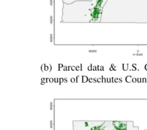
Deschutes County, Oregon is a county with an estimated population of 115,367 people and estimated household population of 45,595 (US Census Bureau 2001). The local county government of Deschutes has parcel data for 70,293 households8. The U.S. Census clas-sifies Deschutes County as mix ofruralandurban(see Table 4 US Census Bureau 2001). The urbanportion of the county is Bend, OR (and few outlying areas around Bend) a city of 52,029 in 2000 (see Table 4: US Census Bureau 2001). Deschutes County is used primarily for it rural nature. A visual portrayal of the household distribution of Portland overlaid on U.S. Census blocks, block groups and tracts may be seen in Figure 3.
Table 4: Deschutes County, Oregon urban/rural classification by the U.S.
Census in 2000
Deschutes County Oregon
Urban: 72,554
Rural: 42,812
Total: 115,367
Figure 3: Deschutes County, Oregon households and polygons (blocks, block groups, and tracts)
(a) Parcel data & U.S. Census 2000 blocks of Deschutes County, OR
(b) Parcel data & U.S. Census 2000 block groups of Deschutes County, OR
(c) Parcel data & U.S. Census 2000 tracts of Deschutes County, OR
7.
Comparison measure
The evaluation of our proposed household location models involves the comparison of two point distributions: that of the observed household distribution and that of the simu-lated household distribution. The literature in applied spatial analysis has tended to focus on the comparison of point distributions over two (or more) time points rather than the comparison of two different point processes. The most common examples are in the eco-logical literature, especially dealing with trees (for a good review see, Perry, Miller, and Enright 2006). However, as we are comparing two different point distributions (i.e., not emanating from a temporal process) we apply Diggle and Chetwynd’s (1991) recommen-dation of using the sum of normalized difference of Ripley’sKstatistic atmbreaks.
D(s) =K1(s)− K2(s)
D=
m ∑
k=1
D(sk) var(D(sk))
(5)
The numerator is sometimes known asDiggle’s D. To test whether the two distributions are different we applyMonte Carlo (MC) tests for spatial patterns(Besag and Diggle 1977).
The MC test employed here consists of ranking the value of a statistic computed on observed data amongst a corresponding set of statistic values generated by random sam-pling from a null distribution. In this case the null distributions are our three proposed models (Uniform, Quasi-random, and Attraction), with our aim being to assess the extent to which the distributions ofD under these models cover theD values of the observed data.
Note that under mild conditions this test determines an exact significance level and that the number of simulations, k, can be quite small.9 We call the resultingp-value
anMC-pvalue. In this research we will not be interested in the MC-pvalue to identify potentially interesting features of data, but to assess the adequacy of the null model to serve as a proxy for the observed distribution. In other words, we are interested in the case when the two distributions are not strongly distinguishable. We will therefore use a standardαlevel of0.05(or0.025 for a two-tailed test) to determine whether the two point processes are sufficiently different to be considered effectively distinct.
8.
Analysis and results
To evaluate our proposed models, we simulate distributions for samples of polygons from each of our three cases, comparing those distributions against the observed data via the MC test of theD statistic (as shown above). Here, we briefly describe software and procedural issues, before turning to our findings.
8.1 Software
All code for this paper was written in theRstatistical programming language (R Devel-opment Core Team 2010). Ris, among other things, a powerful GIS tool (see, Bivand, Pebesma, and Gómez-Rubio 2008). To perform the analysis, functions fromspatstat
(Baddeley and Turner 2005),networkSpatial(Butts and Almquist 2011),splancs
(Rowlingson and Diggle 1993),rgdal(Keitt et al. 2009) andUScensus2000-suite of packages (Almquist 2010) were employed.
8.2 Comparison of point distributions
For each polygon, we perform a MCDtest for each of the three proposed models.10 For each such test, we regard the observed data as adequately covered by the model if theD statistic lies within the central 95% simulation interval produced by the model in ques-tion.11 To assess overall adequacy, we then examine the fraction of areal units for which coverage is adequate. We note that this is a fairly demanding standard of “adequacy,” in that a simulated distribution may prove to be a reasonable approximation of the observed data, while still being statistically distinguishable from it. (We return to this issue below.)
8.2.1 Model adequacy for the test data
Tables 5, 6, and 7 provide the fraction of areal units in each test region for whichD does not differ significantly from each of the three proposed models. Looking across the three regions, we observe immediately that model performance is substantially better for block-level data than for block groups or tracts. This appears to result from the fact that block groups and tracts are not only much larger than blocks, but also substantially
10For computational reasons, we chose to perform our Monte CarloDtest on a population-weighted subsample of areal units from each level for each test case. The sample size for each level/case combination was 100, if 100 units were available; otherwise, all units in the specified level/case combination were used. We did this subsampling routine because each draw of the MC test required considerable computational power and time. Note that standard statistical asymptotics (i.e., central limit theorem) apply here, as the areal units are randomly selected from a well-defined population of such units, and our generalization is to this population.
more heterogeneous; to reproduceDwithin a block group or tract requires the model to correctly reproduce the very considerable variation in population densities observed at the block scale, a feat for which none of the three models are well-prepared. On the other hand, we also see that, of the three models, the Attraction model substantially outperforms its peers on larger areal units. This is because the Attraction model can use boundary information as “clues” about where dense clusters of points might reside, thus recovering some of the underlying heterogeneity. Nevertheless, none of models approach perfect performance for larger areal units.
Table 5: Portland, Oregon: Proportion of blocks nonsignificant under the
MC test performed on the D statistic
Quasi-random Uniform Attraction
Tract 0.00 0.02 0.13
Block Group 0.00 0.14 0.19
Block 0.38 0.56 0.58
Table 6: Irvine, California: Proportion of blocks non-significant under the
MC test performed on the D statistic
Quasi-random Uniform Attraction
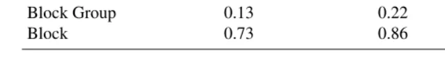
Tract 0.04 0.06 0.22
Block Group 0.13 0.22 0.25
Block 0.73 0.86 0.87
Table 7: Deschutes County, Oregon: Proportion of blocks non-significant
under the MC test performed on the D statistic
Quasi-random Uniform Attraction
Tract 0.00 0.00 0.00
Block Group 0.01 0.04 0.07
For small areal units, on the other hand, performance is quite good: in both Irvine and Deschutes County, approximately 87% of sampled blocks did not differ significantly from the simulated data. Even in Portland, where performance was lowest, the majority of blocks were not statistically distinct from the Attraction model. This suggests that, where one needs a proxy for household location data at the block level, even a very simple model may prove adequate for many applications.
8.2.2 Qualitative comparison
While the Monte Carlo test provides a strict criterion for model adequacy, it is also useful to consider the extent to which theKdistributions produced by the three proposed mod-els qualitatively approach the observed data. As a basic point of comparison, we consider the average squared correlation (R2) between the distribution ofKfunctions for the
sim-ulated household distributions and the observedKfunction. Given the monotone nature of theKfunction, allR2values tend to be high (mean apx 0.98 for tract and block group units, and 0.5 for blocks), but we may directly inspect “typical” cases by selecting the areal unit in each location and scale class for which theR2is at or closest to the median. The resulting curves are shown in Figure 4.
As the figure shows, the qualitative fit of the median case to the data is excellent in Portland, at all scales. Although this may seem surprising in light of the findings of Ta-ble 5, we note that the two procedures involved answer distinct questions: the MC test tells us that deviations from the model are detectable in the Portland case, but the quali-tative examination shows that the behavior of the curves in question are otherwise quite close. By contrast, the fit to the other two cases is not as good; while the overall shape of each curve tracks the data, the magnitudes are plainly off for larger areal units. At the block level, the figure underscores the point that there is considerable variability in the associated distributions, thus contributing to the lack of significant deviations. Taken together with the adequacy results, these results seem to suggest that the proposed models may be good proxies for large-unit behavior in urban areas (even where they are statis-tically distinguishable), and block-level behavior in most areas for use within simulation analysis.
8.2.3 Case study
Figure 4: Kfunction for the median tract/block group/block geography for Portland, OR (a); Irvine, CA (b); and Deschutes County, OR (c)
0.0000 0.0005 0.0010 0.0015
0.0e+00 2.0e−06 4.0e−06 6.0e−06 8.0e−06 1.0e−05 1.2e−05 r K(r) ● ● ● ● Parcel Data Uniform Model Quasi−random Model Attraction Model
Median Density Tract, Portland, OR
0.0000 0.0002 0.0004 0.0006 0.0008 0.0010 0.0012
0e+00 1e−06 2e−06 3e−06 4e−06 5e−06 r K(r) ● ● ● ● Parcel Data Uniform Model Quasi−random Model Attraction Model
Median Density Block Group, Portland, OR
0e+00 1e−04 2e−04 3e−04
0.0e+00 5.0e−08 1.0e−07 1.5e−07 2.0e−07 2.5e−07 3.0e−07 r K(r) ● ● ● ● Parcel Data Uniform Model Quasi−random Model Attraction Model
Median Density Block, Portland, OR
(a)
0.000 0.002 0.004 0.006 0.008 0.010 0.012
0.0000 0.0005 0.0010 0.0015 0.0020 r K(r) ● ● ● ● Parcel Data Uniform Model Quasi−random Model Attraction Model
Median Density Tract, Irvine, CA
0.0000 0.0005 0.0010 0.0015
0e+00 2e−06 4e−06 6e−06 8e−06 1e−05 r K(r) ● ● ● ● Parcel Data Uniform Model Quasi−random Model Attraction Model
Median Density Block Group, Irvine, CA
0.00000 0.00005 0.00010 0.00015 0.00020 0.000250.00030
0.0e+00 5.0e−08 1.0e−07 1.5e−07 r K(r) ● ● ● ● Parcel Data Uniform Model Quasi−random Model Attraction Model
Median Density Block, Irvine, CA (b) 0.0000 0.0005 0.0010 0.0015 0.0020 0.0025 0.0030 0.0035 K(r) ● ● ● ● Parcel Data Uniform Model Quasi−random Model Attraction Model
Median Density Tract, Deschutes County, OR
0e+00 1e−04 2e−04 3e−04 4e−04 5e−04 6e−04 K(r) ● ● ● ● Parcel Data Uniform Model Quasi−random Model Attraction Model
Median Density Block Group, Deschutes County, OR
5.0e−08 1.0e−07 1.5e−07 2.0e−07 K(r) ● ● ● ● Parcel Data Uniform Model Quasi−random Model Attraction Model
Figure 5: Observed household distribution and a single simulation draw of points over tract “009701" in Portland, Oregon for the three base-line models considered in this paper
(a) Parcel Data. (b) Attraction Model
(c) Uniform Model (d) Quasi-random Model.
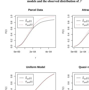
Figure 6 makes it visually apparent that in the chosen tract the Attraction model per-forms significantly better than the other two baseline models. In Figure 7 we see that none of the models capture the fine details of the observed data, although the Attraction model does capture the basic pattern of inhomogeneity in population density throughout the tract. Lastly, we see that in Figure 8 that the Attraction model performs the best on theFstatistic.
9.
Example: Network diffusion over a spatially embedded network
In this paper we have explored the practicality of usingspatial point processesas proxies for human settlement patterns for small areal units. While we anticipate many practical uses for this procedure one particularly salient example comes from the social network literature. Anetwork(orgraph) in mathematical language is a relational structure con-sisting of two elements: a set ofverticesornodes(here used interchangeably), and set of vertex pairs representingtiesoredges(i.e., a “relationship" between two vertices). For-mally, this is often represented asG= (V, E), whereV is thevertex setandEis theedge set. IfGis undirected, then edges consist of unordered vertex pairs, with edges consisting of ordered pairs in the directed case. IfGis directed then the network consists of ordered pairs (i, j).12
Butts (2003) introduced a model for simulating large scale geographically embed-ded networks, thespatial Bernoulligraphs. These models require a rather high level of precision for both simulation and estimation (i.e., they require the researcher to assign a location to every individual in the network of interest, which is not possible when using aggregated spatial data such as that provided by the U.S. Census). When exact measure-ment of individual positions is not practical, point process models like those introduced here may be employed to approximate locations based on spatial aggregates. Given a realization from such a point process, we can in turn simulate the associated network (if necessary, repeating the process multiple times to average over spatial uncertainty). From simulated population networks we can predict a range of structural properties (e.g., clus-tering, degree, etc.) and correlate these attributes with observed demographic and social effects (e.g., income or crime) for predictive or exploratory purposes. These large-scale networks also allow a researcher to study the behavior of population processes that might occur via non-random mixing, for example the diffusion of sexually transmitted infec-tions, disease epidemics, information transmission, or ideas.
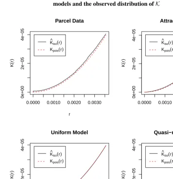
Figure 6: Comparison ofKfunction: Comparison of the three baseline
models and the observed distribution ofK
0.0000 0.0010 0.0020 0.0030
0e+00 2e−05 4e−05 Parcel Data r K ( r )
K^iso(r)
Kpois(r)
0.0000 0.0010 0.0020 0.0030
0e+00 2e−05 4e−05 Attraction Model r K ( r )
K^iso(r)
Kpois(r)
0.0000 0.0010 0.0020 0.0030
0e+00 2e−05 4e−05 Uniform Model r K ( r )
K^iso(r)
Kpois(r)
0.0000 0.0010 0.0020 0.0030
0e+00 2e−05 4e−05 Quasi−random Model r K ( r )
K^iso(r)
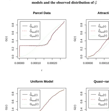
Figure 7: Comparison ofGfunction: Comparison of the three baseline
models and the observed distribution ofG
0.00000 0.00010 0.00020
0.0 0.2 0.4 0.6 0.8 Parcel Data r G ( r )
G^km(r)
G^bord(r)
Gpois(r)
0.00000 0.00010 0.00020
0.0 0.2 0.4 0.6 0.8 Attraction Model r G ( r )
G^km(r)
G^bord(r)
Gpois(r)
0.00000 0.00010 0.00020 0.00030
0.0 0.2 0.4 0.6 0.8 Uniform Model r G ( r )
G^km(r)
G^bord(r)
Gpois(r)
0.00000 0.00010 0.00020 0.00030
0.0 0.2 0.4 0.6 0.8 Quasi−random Model r G ( r )
G^km(r)
G^bord(r)
Figure 8: Comparison ofFfunction: Comparison of the three baseline
models and the observed distribution ofF
0e+00 2e−04 4e−04
0.0 0.2 0.4 0.6 0.8 1.0 Parcel Data r F ( r )
F^km(r)
Fpois(r)
0e+00 1e−04 2e−04 3e−04 4e−04
0.0 0.2 0.4 0.6 0.8 1.0 Attraction Model r F ( r )
F^km(r)
Fpois(r)
0.00000 0.00010 0.00020
0.0 0.2 0.4 0.6 0.8 Uniform Model r F ( r )
F^km(r)
Fpois(r)
0.00000 0.00010 0.00020
0.0 0.2 0.4 0.6 0.8 Quasi−random Model r F ( r )
F^km(r)
Fpois(r)
9.1 Spatial Bernoulli Graphs and Simulation
It is well-known that the marginal probability of a tie between two persons declines with geographical distance for a broad range of relationships (e.g., Bossard 1932; Festinger, Schachter, and Back 1950; Hägerstrand 1966; Freeman, Freeman, and Michaelson 1988; Latané, Nowak, and Liu 1994; McPherson, Smith-Lovin, and Cook 2001). Given the highly structured nature of human settlement patterns, this relationship is a powerful de-terminant of social structure (Mayhew 1984b); indeed, at large geographical scales, much of the information content in network structure must be predictable by spatial factors un-der fairly weak conditions (Butts 2003). Since much is known regarding the distributions of populations in space, geography is thus a highly effective starting point for the model-ing of large-scale social networks.
The most basic family of spatial network models is that of the spatial Bernoulli graphs. Here, we define the spatial Bernoulli graphs in the manner of Butts and Ac-ton (2011). Consider a set of vertices,V, which are spatially embedded with a distance matrixD∈[0,1)N×N. LetGbe a random graph onV, with stochastic adjacency matrix Y ∈ {0,1}N×N. Then the probability mass function (pmf) ofGgivenDis:
Pr(Y =y|D,Fd) = ∏
{i,j}
B(yij| Fd(dij)) (6)
whereBis the Bernoulli pmf, andFd: [0,∞)→[0,1]is thespatial interaction function, or SIF. The SIF controls the underlying structure of the network and is thus a key com-ponent within this family of models. Specifically, the SIF relates distance to the marginal tie probability. Empirically it appears that many real-world social networks have an SIF where the marginal tie probability decays monotonically with distance, declining quickly for short distances but exhibiting an extremely long tail (see, Butts 2003). One plausible functional form for a social network SIF having these properties is the power law, i.e.
Fd(x) = pd
(1 +αx)γ (7)
E[Yij]∝P(i)P(j)Fd(d(i, j)), (8)
whereP(x)is theinteraction potentialof elementx, andFdis the SIF.
9.1.1 Simulation procedure
Here we will follow the simulation procedure of Butts et al. (2012), noting that to simulate a spatial Bernoulli graph we must have a point location for each node in the graph. We begin with GIS-based population data for a given spatial area, using polygons and block-level demographics from the U.S. Census. Next, we place individuals in their respective blocks using an inhomogenous Poisson point process model as discussed in Section 4.3. We then overlay a network on the individuals, employing the spatial Bernoulli models (discussed in Section 9.1) and informed by a historical social friendship network (param-eter estimation comes from Butts 2003). This “social friendship" relation, and can be thought of as a locally sparse relation with a fairly long tail (declining as approximately d−2.8for large distances). The parametric form is a power law, with parameters (0.533,
.032, 2.788). (For a visualization of this SIF see Figure 9).
9.2 Network diffusion
To demonstrate one illustrative application of our model, we simulate anetwork diffusion
process over spatially simulated network and observe the rate of transmission. We will begin with a single event (e.g., the introduction of a rumor to be spread, an emergency event about which individuals may disseminate information, or the appearance of a highly communicable disease within a population). The initial signal (or seed) will be provided to all individuals withinXdistance of the primary event. In this simulation study we will employ a standard network diffusion model (Frambach 1993).13 The Poisson diffusion
model operates in the following way: At arbitrary timet, every vertex is either “infected” (i.e., has been reached by the diffusion process), or “uninfected” (i.e., has not yet been reached). Once infected, a vertex (v) initiates an infection event for each of his or her out-neighbors (vn) which occurs at timet+X (whereX ∼eλvvn)). An uninfected vertex becomes infected at the time of its first infection event; subsequent infection events have no effect. The simulation terminates when all reachable vertices have been infected (all times are given relative to the initiation of the diffusion process.) As the above suggests, the speed of the diffusion process is governed by the edge-specific rates,λ. For illustrative purposes we treatλas equal for all edges, although this assumption can easily be relaxed in substantive applications.
Figure 9: SIF for Festinger’s (1954) social friendship data
0 20 40 60 80 100
0.0
0.1
0.2
0.3
0.4
0.5
Distance
Fd
(
x
)
=
0.533
(
1
+
0.032
x
)
2.788
9.3 Simulated diffusion over Portland, OR
epidemiological context), and/or may identify relatively isolated subpopulations in need of additional connectivity (e.g., in the context of warnings and alerts).
The case illustrated here is a very simple one, and highly abstract; nonetheless, it demonstrates the manner in which a point process model like those described here can facilitate large-scale modeling and analysis from spatially aggregated demographic data. Spatial network models, like other models that require point locations for simulation or estimation procedures, could greatly benefit from the methodology discussed in this paper. As the capability and need for micro-level simulation of population processes continue to grow, we expect a corresponding growth in the need for effective and efficient methods for imputing point locations of households, individuals, or other social units.
Figure 10: Network diffusion process over a spatial Bernoulli graph
simulated for Portland, OR
10.
Conclusion and discussion
In this paper we have set forth a basic problem that exists because of the spatial aggrega-tion of large scale administrative data such as the U.S. Census: the simulaaggrega-tion of house-hold locations within small areal units. The placement of househouse-holds (or individuals) is important for many social and demographic processes and the ability to map households within a given polygonal boundary is potentially important for micro-social processes such as transmission of disease between households, daily mobility patterns, or patterns of interpersonal contact. When dealing with processes that require modeling interaction directly (e.g., social networks) one often has need of a specific location for individuals or households. One illustrative example of such a process was shown in Section 9, and myriad generalizations are possible.
As a starting point for dealing with the household distribution problem, we proposed three simple, scalable point process models that can be used with little input by the ana-lyst. Testing against parcel data showed that at the block level all three models perform reasonably well, but the Attraction model typically outperforms the Quasi-random and the Uniform model in tract and block group levels (sometimes by as much as 16 percent). Since the Attraction model performs as well or better than the other two models, we ad-vocate that for household simulation one should in general use the Attraction model. The Attraction model also has the advantage of being able to take into account macro-level patterns such as roads or waterways, unlike the Uniform and Quasi-random models (Fig-ure 6(b)).
11.
Acknowledgments
References
Almquist, Z.W. (2010). US Census spatial and demographic data in R: The UScensus2000 suite of packages.Journal of Statistical Software37(6): 1–31.
Baddeley, A. and Turner, R. (2005). Spatstat: An R package for analyzing spatial point patterns.Journal of Statistical Software12(6): 1–42.
Besag, J. and Diggle, P.J. (1977). Simple Monte Carlo tests for spatial pattern. Jour-nal of the Royal Statistical Society: Series C (Applied Statistics). 26(3): 327–333. doi:10.2307/2346974.
Binka, F.N., Indome, F., and Smith, T. (1998). Impact of spatial distribution of permethrin-impregnated bed nets on child mortality in rural northern Ghana. The American Journal of Tropical Medicine and Hygiene59(1): 80–5.
Bivand, R.S., Pebesma, E.J., and Gómez-Rubio, V. (2008).Applied Spatial Data Analysis with R. New York, NY: Springer.
Bossard, J.H.S. (1932). Residential propinquity as a factor in marriage selection. Ameri-can Journal of Sociology38(2): 219–224. doi:10.1086/216031.
Burian, S.J., Brown, M.J., and Velugubantla, S.P. (2002). Building height characteristics in three U.S. cities. In: Proceedings of the American Meteorological Society’s Fourth Symposium on the Urban Environment.
Butts, C.T. (2003). Predictability of large-scale spatially embedded networks. In: Breiger, R.L., Carley, K.M., and Pattison, P. (eds.). Dynamic Social Network Modeling and Analysis: Workshop Summary and Papers. National Academies Press: 313–323. Butts, C.T. (2008). Diffusion: Tools for simulating network diffusion processes.
[elec-tronic resource]. R package version 0.5. http://erzuli.ss.uci.edu/R.stuff.
Butts, C.T. and Acton, R.M. (2011). Spatial modeling of social networks. In: Nyerges, T., Couclelis, H., and McMaster, R. (eds.).The Sage Handbook of GIS and Society Research. Thousand Oaks, CA: SAGE Publications: 222–250.
Butts, C.T., Acton, R.M., Hipp, J.R., and Nagle, N.N. (2012). Geographical variablity and network structure.Social Networks34(1): 82–100.doi:10.1016/j.socnet.2011.08.003. Butts, C.T. and Almquist, Z.W. (2011). NetworkSpatial: Tools for the generation and analysis of spatially-embedded networks. [electronic resource]. R package version 0.6. http://erzuli.ss.uci.edu/R.stuff.
Applications. Springer/Birkhüse: 129–152.
Davis, H.L. (1976). Decision making within the household. Journal of Consumer Re-search2(4): 241–260.doi:10.1086/208639.
Diggle, P.J. (2003).Statistical Analysis of Spatial Point Patterns. Oxford, UK: A Hodder Arnold Publication, 2nd ed.
Diggle, P. and Chetwynd, A. (1991). Second-order analysis of spatial clustering for inho-mogeneous populations.Biometrics47(3): 1155–1163.doi:10.2307/2532668. Festinger, L. (1954). A theory of social comparison processes. Human Relations7(2):
117–140.doi:10.1177/001872675400700202.
Festinger, L., Schachter, S., and Back, K. (1950). Social Pressures in Informal Groups: A Study of Human Factors in Housing. Palo Alto, CA: Stanford University Press. Fox, J., Rindfuss, R., Walsh, S., and Mishra, V. (eds.) (2003).People and the Enviroment:
Approaches for Linking Household and Community Surveys to Remote Sensing and GIS. New York, NY: Kluwer Academic Publisher.
Frambach, R.T. (1993). An integrated model of organizational adoption and diffusion of innovations. European Journal of Marketing 27(5): 22–41. doi:10.1108/03090569310039705.
Freeman, L.C., Freeman, S.C., and Michaelson, A.G. (1988). On human social intel-ligence. Journal of Social Biological Structures11(4): 415–425. doi:10.1016/0140-1750(88)90080-2.
Freeman, L.C. and Sunshine, M.H. (1976). Race and intra-urban migration.Demography
13(4): 571–575.doi:10.2307/2060511.
Gentle, J.E. (1998).Random Number Generation and Monte Carlo Methods. New York, NY: Springer.
Gibson, C.C., Ostrom, E., and Ahn, T.K. (2000). The concept of scale and the hu-man dimensions of global change: A survey. Ecological Economics32(2): 217–239. doi:10.1016/S0921-8009(99)00092-0.
Glaz, J., Pozdnyakov, V., and Wallenstein, S. (eds.) (2009). Applications of Spatial Scan Statistics: A Review. Statistics for Industry and Technology. Boston, MA: Springer/Birkhüse.
Goodchild, M.F. (2007). Citizens as sensors: The world of volunteered geography.
GeoJournal69(4): 211–221. doi:10.1007/s10708-007-9111-y.
districts.Population and Development Review27(4): 713–738. doi:10.1111/j.1728-4457.2001.00713.x.
Hägerstrand, T. (1966). Aspects of the spatial structure of social communication and the diffusion of information.Papers in Regional Science16(1): 27–42.
doi:10.1007/BF01888934.
Harris, C.D. (1943). Suburbs. American Journal of Sociology49(1): 1–13.doi:10.1086/ 219303.
Haynes, K.E. and Fortheringham, A.S. (1984). Gravity and spatial interaction models, Vol. 2 of Scientific Geography. Beverly Hills: Sage publications.
Hipp, J.R., Faris, R.W., and Boessen, A. (2012). Measuring ‘neighbor-hood’: Constructing network neighborhoods. Social Networks 34(1): 128–140. doi:10.1016/j.socnet.2011.05.002.
Keitt, T.H., Bivand, R., Pebesma, E., and Rowlingson, B. (2009). rgdal: Bindings for the geospatial data abstraction library. http://CRAN.R-project.org/package=rgdal
(R package version 0.6-21).
Kulldorff, M. (1997). A spatial scan statistic. Communication Statistics26(6): 1481– 1496.doi:10.1080/03610929708831995.
Latané, B., Nowak, A., and Liu, J.H. (1994). Measuring emergent social phenom-ena: Dynamism, polarization, and clustering as order parameters of social systems.
Behavioral Science39(1): 1–24.doi:10.1002/bs.3830390102.
Martin, D. and Bracken, I. (1991). Techniques for modeling population-related raster databases.Environment and Planning A23(7): 1069–1075.doi:10.1068/a231069. Mayhew, B.H. (1984a). Baseline models of sociological phenomena. Journal of
Mathe-matical Sociology9(4): 259–281.doi:10.1080/0022250X.1984.9989948.
Mayhew, B.H. (1984b). Chance and necessity in sociological theory. Journal of Mathe-matical Sociology9(4): 305–339.doi:10.1080/0022250X.1984.9989953.
McC. Netting, R., Wilk, R.R., and Arnould, E.J. (eds.) (1984).Households: Comparative and Historical Studies of the Domestic Group. Berkeley, CA: University of California Press.
McPherson, M., Smith-Lovin, L., and Cook, J.M. (2001). Birds of a feather: Homophily in social networks. Annual Review Sociology 27(1): 415–444. doi:10.1146/annurev.soc.27.1.415.
international: Version 6.1 [machine-readable database]. Minneapolis: University of Minnesota.
Naus, J.I. (1965). Clustering of random points in two dimensions. Biometrica52(1/2): 263–267.doi:10.2307/2333829.
Openshaw, S. (1984).The Modifiable Areal Unit Problem. Norwich: Geo Books. Perry, G.L.W., Miller, B.P., and Enright, N.J. (2006). A comparison of methods for the
statistical analysis of spatial point patterns in plant ecology.Plant Ecology187(59-82). doi:10.1007/s11258-006-9133-4.
R Development Core Team (2010). R: A language and environment for statistical com-puting. Vienna, Austria: R Foundation for Statistical Comcom-puting.
http://www.R-project.org. ISBN 3-900051-07-0.
Reibel, M. (2007). Geographic information systems and spatial data processing in de-mography: A review. Population Research and Policy Review 26(5-6): 601–618. doi:10.1007/s11113-007-9046-5.
Ripley, B.D. (1988). Statistical Inference for Spatial Processes. Cambridge: Cambridge University Press.
Rowlingson, B.S. and Diggle, P.J. (1993). Splancs: Spatial point pattern analysis code in s-plus. Lancaster, UK: Lancaster University.
Salathé, M. and Jones, J.H. (2010). Dynamics and control of diseases in net-works with community structure. PLoS Computational Biology 6(4): e1000736. doi:10.1371/journal.pcbi.1000736.
Short, M.B., Brantingham, P.J., Bertozzi, A.L., and Tita, G.E. (2010). Dissipation and displacement of hotspots in reaction-diffusion models of crime. Proceedings of the National Academy of Sciences.
Snyder, J.P. (1987). Map projections – a working manual. Washington, D.C.: United States Government Printing Office. (U.S. Geological Survey Professional Paper). Stoyan, D., Kendall, W.S., and Mecke, J. (1987). Stochastic Geometry and Its
Applica-tions. New York: Wiley, 2nd ed.
Theobald, D.M. (2004). Placing exurban land-use change in a human modification frame-work.Frontiers in Ecology and the Enviroment2(3): 139–144.doi:10.2307/3868239. Tobler, W. (1979). Smooth pycnophylactic interpolation for geographic regions.Journal
U.S. Census Bureau. U.S. Census Bureau.
Voss, P.R. (2007). Demography as a spatial social science. Population Research and Policy Review26(5-6): 457–476.doi:/10.1007/s11113-007-9047-4.