Evaluation of Several Methods of Predicting Historic Water Table Levels

(1)

ABSTRACT

SEVERSON, ERIK. Evaluation of Several Methods of Predicting Historic Water Table Levels (Under the direction of Dr. David Lindbo)

Redoximorphic features (iron depletions) and their location in the soil indicate seasonal high water tables, which are the critical factors in siting onsite wastewater disposal systems. According to rule “.1942 Soil Wetness” (15NCAC 18A, 2005), soil wetness conditions are determined by soil morphology is the first occurrence (≥ 2% by volume) of chroma 2 or less iron depletions Soil wetness regulations have created a need for more research in soil hydrology.

The general objective of this study is to define relationships between soil

morphology and water table in order to confirm or establish three water table monitoring and interpretation procedures; Calibration, Threshold, and Weighted Rainfall Index (WRI) methods. These methods are used or recognized by state regulatory agencies. Specific objectives of this study are; 1. to evaluate relationships between observed water table dynamics and soil morphology; and 2. to compare NCDENR methods of

determining soil wetness to the soil morphological indicator of soil wetness

Three experimental sites on the Lower Coastal Plain (LCP) were established to encompass different soil types and properties. The Richlands Site contained coarse-loamy textured soils, the Vanceboro Site contained clayey soils, and the Cool Springs Site contained sandy soils. Automated recording water table level wells monitored a total of 20 plots in transects of clayey Aquic Hapludults (Craven) and Aeric Paleaquults (Lenoir); sandy Typic Udipsamments (Tarboro and its wet-end variant) and Aquic Udipsamments (Seabrook); and coarse-loamy Aquic Paleuduults (Foreston and its wet-end variant) and Aeric Paleaquults (Stallings) for over 365 days. These water table and on-site rainfall data (one rain gauge was located at each site) were used as input

information for the hydrologic model DRAINMOD (Skaggs, 1978) to independently predict 30-yr historic water table levels for each soil. Using long-term weather data, soil wetness conditions for each method were determined for each of the 20 plots.

(2)

accordance to rule .1942 (f) (NCAC 2005). Once the modelwas calibrated, long-term water table levels were predicted using historic (+30 yr) rainfall data from the nearest weather station in order to determine the probabilitythat a site will be saturated for a 14-d continuous period with a recurrence frequency of 30%. These values were then related to the depth of the first occurrence of three types of redox features (iron concentrations, ≤ 2 and ≤ 3 chroma iron depletions).

The Threshold method is a modified form of the Threshold Wetland Simulation (TWS) as reported by Hunt et al., 2001. The requirements for obtaining the soil wetness conditions by the Threshold method were the same as those for the calibration method (14-d continuous period with a recurrence frequency of 30%). This method uses one representative soil in that can be extrapolated to other similar soils. The depths of soil wetness conditions predicted by this method were never more than 12 cm different from those wetness conditions predicted by the Calibration method at all sites.

The soil wetness conditions determined by the WRI method is a sliding scale of saturation durations based on monitored rainfall data only. Those values that were obtained were variable within each plot, ranging (at all sites) from ponded conditions (0 cm) to 65 cm below the surface. Therefore, the wetness conditions predicted by this method are split into two groups, WRI-H (water table depth of 0 cm) and WRI-L (water table depth of 65 cm) for each plot. In the case of multiple years of analysis, the

shallowest depth predicted by this method is the soil wetness condition (15NCAC 18A .1942, 2005). The soil wetness condition acquired by the WRI method could not be determined for every year of analysis due to lack of required rainfall.

The Calibration, Threshold, and WRI methods of determining soil wetness conditions have specific relationships with the soil morphological indicator of wetness (chroma ≤ 2 depletions). For all the soils at the Richlands site and the Lenoir soils of the Vanceboro site, wetness conditions predicted by the different methods (except WRI-H) were higher in the soil profile than the morphology suggests. The level of soil wetness conditions predicted by all methods (except WRI-H) for the Craven soils of the

(3)

the Seabrook soils of the Cool Springs site matched the level of the chroma ≤ 2 color occurrence.

Soil wetness conditions depths predicted by the Calibration and Threshold

methods related best with the depth to different redox features in the following soils. For all soil plots of the Richlands site, the average depth to soil wetness conditions

determined by the Calibration method (43 cm) related best with average depth of first occurrence of iron concentrations (43 cm). The average depth of Calibration wetness condition (30 cm) related best with average depth of ≥3 depletions (32 cm) in the Lenoir soils. There was not a consistent relationship in the Aquic Hapludults between the average calibrated soil wetness condition (102 cm) and the average depth of chroma ≤ 2 depletions (52 cm). The average depth to chroma ≥3 depletions (112 cm) of the wet and dry end of the Tarboro soils related best with the average depth of soil wetness

(4)

EVALUATION OF SEVERAL METHODS OF PREDICTING

HISTORIC WATER TABLE LEVELS

By

Erik D. Severson

A thesis submitted to the Graduate Faculty of

North Carolina State University

in partial fulfillment of the

requirements for the Degree of

Masters of Science

SOIL SCIENCE

Raleigh

2005

APPROVED BY:

Dr. D.L Lindbo (chair)

Dr. M.J. Vepraskas (co-chair)

(5)

BIOGRAPHY

(6)

ACKNOWLEDGEMENTS

The author wishes to express his appreciation to his committee members: Dr. David Lindbo, chair, Dr. Michael J. Vepraskas, Dr. Robert Evans, and Dr. Aziz Amoozegar for their guidance and assistance in this research. The author could not have had a better advisor than Dr. David Lindbo. Special thanks goes to Dr. Steve Broome for providing a home for the author at NCSU upon his arrival. I have much enjoyed working with these respected individuals. I want to thank the technicians and regional soil specialists for their valuable help. These individuals include but are not limited to Mr. Roland Coburn for his invaluable instrumentation assistance, Mr. Charley Humphrey for his data collection, Mr. Tripp Cox for digging superior soil pits and redox probe construction techniques, Mr. Alex Adams and Mr. Charles Karpa for their technical knowledge on rainfall measurement apparatus, Mr. Chris Niewhoener for his assistance in physical properties and water flow measurements, Mr. Rob Austin for his GIS expertise, and Miss Erin Bryan for her data collection. I also want to thank the landowners and their liaisons, for without their help, this research would not be possible. These individuals include Talmadge Haddock, Danny Baysden, and Jeff Hall of the Cool Springs Environmental Center. Individuals from the governmental sector aided in this research include Mr. Walter Geise and Haywood Pittman of Onslow County Health

(7)

TABLE OF CONTENTS

LIST OF TABLES ……….vii

LIST OF FIGURES ………...xii

1. INTRODUCTION………...1

2. LITERATURE REVIEW………5

2.1 Soil Morphology……….5

2.1.1 Soil Color………....6

2.1.2 Redoximorphic Features………..7

2.2 Redox chemistry and morphology ………9

2.3 Redox feature formation ………...11

2.4 Seasonal High Water Table Estimations ……….12

2.5 Misinterpretation Possibilities……….13

2.6 Water table- Redox feature correlations ……….15

2.7 Computer Simulated Water Tables ………...17

3. MATERIALS AND METHODS ………...20

3.1 Experimental Sites………20

3.1.1 Richlands Site………22

3.1.2 Vanceboro Site………..………25

3.1.3 Cool Springs Site………28

3.2 Water Table Fluctuations………..30

3.3 Rainfall………..31

3.4 Temperature………..32

3.5 Redox Potential and soil pH………..32

3.6 Soil Sampling………33

3.7 Water Movement………...33

3.8 Modeling Water Tables….………34

3.9 DRAINMOD……….35

3.9.1 Model……….39

3.9.2 Assumptions………45

3.10 Methods of Soil Wetness Conditions Determination……….45

3.10.1 Calibration Method………..45

3.10.2 Threshold Stimulus Method……….49

3.10.3 Interpretation Method for Direct Monitoring Procedure………….58

4. RESULTS AND DISCUSSION ………...62

(8)

4.2 Evaluation of the Calibration Method ………...64

4.3 Richlands Site………...65

4.3.1 General Conditions………...65

4.3.2 Foreston Soils………65

4.3.3 Wet Foreston Soils……….70

4.3.4 Stallings………....74

4.3.5 Summary of the Richlands Site……….78

4.4 Vanceboro Site ……….80

4.4.1 General Conditions………80

4.4.2 Craven Soils………...81

4.4.3 Lenoir Soils………85

4.4.4 Summary of the Vanceboro Site………89

4.5 Cool Springs Site………..92

4.5.1 General Conditions………92

4.5.2 Tarboro Soil………...93

4.5.3 Wet Tarboro Soils ………...97

4.5.4 Seabrook Soils………...………..101

4.5.5 Summary of the Cool Springs Site………...105

5. CONCLUSIONS ………...108

6. REFERENCES……….113

APPENDIX A MEASURED RAINFALL FOR ALL SITES………...118

APPENDIX B SOIL PROFILE DESCRIPTIONS FOR ALLPLOTS IN ALL EXPEPERIMENTAL SITES ………...121

B.1 Richlands Site……….122

B.2 Vanceboro Site………...128

B.3 Cool Springs Site………134

APPENDIX C SAMPLE OF DRAINMOD INPUTS FOR THE SOILS AT ALL OF THE EXPERIMENTAL SITES………139

C.1 DRAINMOD inputs for plot 2 Fo at the Richlands site ………140

C.2 DRAINMOD inputs for plot 2 wFo at the Richlands site ……….146

C.3 DRAINMOD inputs for plot 2 St at the Richlands site……….152

C.4 DRAINMOD inputs for plot 2 Cr at the Vanceboro site………...158

C.5 DRAINMOD inputs for plot 2 Le at the Vanceboro site ………..164

C.6 DRAINMOD inputs for plot Ta at the Cool Springs site ……….170

C.7 DRAINMOD inputs for plot 1 wTa at the Cool Springs site ………....176

(9)

APPENDIX D

MEASURED HYDROGRAPHS AND REDOX FEATURE DEPTHS FOR ALL PLOTS AT EVERY STUDY SITE……….188

APPENDIX E

OBSERVED AND PREDICTED HYDROGRAPHS OBTAINED BY THE CALIBRATION METHOD FOR ALL PLOTS AT EVERY STUDY SITE ……….199

APPENDIX F

COMPARATIVE HYDROGRAPHS OF OBSERVED AND

SIMULATED DATA FOR VARYING THRESHOLD LEVELS FOR SELECTED PLOTS AT ALL STUDY SITES………...210

APPENDIX G

HISTORIC SOIL WETNESS CONDITIONS OBTAINED BY THE WRI METHOD FOR SELECTED PLOTS AT EVERY STUDY SITE ………222

APPENDIX H

SATURATED HYRDAULIC CONDUCTIVITY FOR SELECTED PLOTS AT THE RICHLANDS AND VANCEBORO SITES………228

APPENDIX I

15A NCAC 18A .1942 SOIL WETNESS CONDITIONS ………..231

APPENDIX J

CALIBRATION METHOD SUCCESS CRITERIA FOR ALL PLOTS AT ALL

(10)

List of Tables

Table 3.1 Sample of raw data to create .OBS files in DRAINMOD………..39

Table 3.2 Sample columnar raw rainfall data to be converted into appropriate

DRAINMOD format ………..40

Table 3.3 Sample raw temperature data to be converted into appropriate

DRAINMOD format ………..40

Table 3.4 Drainage input parameters used in the Calibration Method for the Richlands, Vanceboro, and Cool Springs sites, obtained by calibration to represent the best relationship between observed and predicted

water tables of all soil plots………44

Table 3.5 Long-term Threshold Levels and their corresponding drain spacings that are used to obtain hydrographs that are ‘approximately equal to’, ‘wetter’ and ‘drier’ than the measured hydrographs by the Threshold Method for the for the Foreston/ wet Foreston plots at the Richlands Site………..55

Table 3.6 Long-term Threshold Levels and their corresponding drain spacings that are used to obtain hydrographs that are ‘approximately equal to’, ‘wetter’, and ‘drier’ than the measured hydrographs by the Threshold Method for the for the Craven plots at the Vanceboro site ………56

Table 3.7 Long-term Threshold Levels and their corresponding drain spacings that are used to obtain hydrographs that are ‘approximately equal to’, ‘wetter’ and ‘drier’ than the measured hydrographs by the Threshold Method for the for the Lenoir plots at the Vanceboro site ………56

Table 3.8 Long-term Threshold Levels and their corresponding drain depths that are used to obtain hydrographs that are ‘approximately equal to’, ‘wetter’ and ‘drier’ than the measured hydrographs by the Threshold Method for the for the soils of the Cool Springs site ………57

Table 3.9 Parameters for determining the soil wetness condition by the WRI

Method………60

Table 4.1 Soil morphological features for the Foreston 1 plot………66

(11)

Table 4.3 Saturation durations at the level of redox feature occurrence for the

monitored period for the Foreston plots of all three transects………67

Table 4.4 Saturation durations at the level of redox feature occurrence for the simulated, long-term period for the Foreston plots of all three

transects………..67

Table 4.5 Soil wetness conditions determined by observation and by the three methods of using DRAINMOD simulated data for the Foreston plots… 68

Table 4.6 Soil morphological features for the wet Foreston 1 plot……….70

Table 4.7 Redox features and their depths in the wet Foreston plot....………...71

Table 4.8 Saturation durations for the Monitored period of the wet Foreston

Plots………71

Table 4.9 Saturation durations for the long-term simulated record of the wet

Foreston plots ………...72

Table 4.10 Soil wetness conditions determined by observation and by the three methods of using DRAINMOD simulated data for the wet Foreston plots ………...72

Table 4.11 Soil morphological features for the Stallings1 plot……….74

Table 4.12 Redox features and their depths in the Stallings plots………..…..75

monitored period for the Stallings plots of all three transects………76

simulated period for the Stallings plots of all three transects …………....76

Table 4.15 Soil wetness conditions determined by observation and by the three methods of using DRAINMOD simulated data for the Stallings plots…. 77

Table 4.16 Average depths of all redox feature by soil type……….79

(12)

Table 4.18 Average saturation durations during the simulated period of all plots...80

Table 4.19 Summary of average soil wetness conditions determined by monitored and DRAINMOD simulated data, by soil type ...80

Table 4.20 Soil morphological features for the Craven 1 plot...81

Table 4.21 Redox features depths of the Craven plots...82

monitored period for the Craven plots ...82

simulated, long-term period for the Craven plots ...83

Table 4.24 Soil wetness conditions determined by observation and by the three

methods of using DRAINMOD simulated data for the Craven plots…... 83

Table 4.25 Soil morphological features for the Lenoir 1 plot...86

Table 4.26 Redox features and their depths in the Lenoir plots………...86

Table 4.27 Saturation durations for the Monitored period of the Lenoir plots...87

Table 4.28 Saturation durations for the long-term simulated record of the Lenoir Plots ...87

Table 4.29 Soil wetness conditions determined by observation and by the three methods of using DRAINMOD simulated data for the Lenoir plots ...88

Table 4.30 Average depths of all redox features by soil type...90

Table 4.31 Average saturation durations at the level of redox feature occurrence for the Monitored period of all plots of the Vanceboro site ...90

Table 4.32 Average saturation durations during the simulated period of all plots… .91

Table 4.33 Summary of average soil wetness conditions determined by monitored and DRAINMOD simulated data, by soil type ...91

Table 4.34 Soil morphological features for the Tarboro plot………. 93

(13)

monitored period for the Tarboro plots of all three transects ...94

simulated, long-term period for the Tarboro plots of all three transects....95

Table 4.38 Soil wetness conditions determined by observation and by the three

methods of using DRAINMOD simulated data for the Tarboro plot…… 95

Table 4.39 Soil morphological features for the wet Tarboro 1 plo...97

Table 4.40 Redox features and their depths in the wet Tarboro plots………..98

Table 4.41 Saturation durations for the Monitored period of the wet Tarboro plots...98

Table 4.42 Saturation durations for the long-term simulated record of the wet

Tarboro plots ...99

Table 4.43 Soil wetness conditions determined by observation and by the three methods of using DRAINMOD simulated data for the wet

Tarboro plots ………...99

Table 4.44 Soil morphological features for the Seabrook 1 plot ...101

Table 4.45 Redox features and their depths in the Seabrook plots...102

monitored period for the Seabrook plots of all three transects ...103

simulated period for the Seabrook plots of all three transects ...103

Table 4.48 Soil wetness conditions determined by observation and by the three methods of using DRAINMOD simulated data for the

Seabrook plots ...103

Table 4.49 Average depths of all redox features for all plots of the Cool Springs Site ...105

Table 4.50 Average saturation durations at the level of redox feature occurrence for the Monitored period of all plots ...106

Table 4.51 Average saturation durations during the simulated period of all plots… 106

(14)

Table H.1 Saturated hydraulic conductivities of the soils in transect 2 of the

Richlands site ...223

Table H.2 Saturated hydraulic conductivities of the soils in transect 2 of the

Vanceboro site ...223

Table J.1 A summary of average absolute deviations used for comparison of

(15)

List of Figures

Figure 3.1 Map of eastern NC showing the three experimental sites on the

Lower Coastal Plain. Richlands site was in Onslow Co., and the Cool Springs and Vanceboro sites were both in Craven Co (Map

taken from Daniels et al., 1999) ...20

Figure 3.2 Generalized layout of soil plots (octagons) along transects and

their landscape position ...21

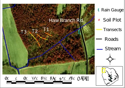
Figure 3.3 Layout of the Richlands site showing relative plot locations and their relationships between certain features such as roads, streams

and the rain gauge ...22

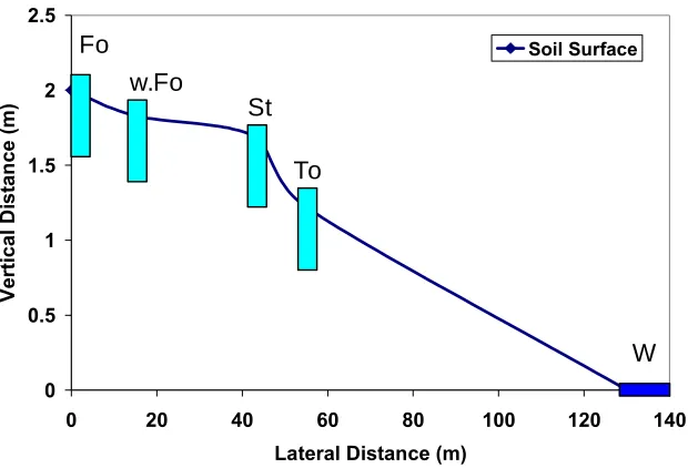
Figure 3.4 Relative elevation of the Foreston (Fo), wet Foreston (w.Fo.), Stallings (St), and Torhunta (To) soil plots along a transect 1 of the

Richalnds site ...24

Figure 3.5 Layout of Vanceboro site showing plot locations along transects and their relationships between certain features such as roads, streams,

and the rain gauge ...26

Figure 3.6 Relative elevations of Craven (Cr), Lenoir (Le), and Leaf (La) soil

plots and natural stream (W) along transect 2 of the Vanceboro site…....27

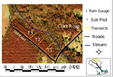
Figure 3.7 Layout of the Cool Springs site showing relative plot locations and their relationships between certain features such as roads,

backswamp, and the rain gauge ...29

Figure 3.8 Relative elevation of six soil plots along a transect 1 of the Cool

Springs site ...30

Figure 3.9 Example of a successful calibration for the Foreston 1 plot...47

Figure 3.10 Wetland hydrology output file (.WET) example for the Fo 1 plot...48

Figure 3.11 Comparative hydrographs of observed vs. ‘wetter’ simulated

hydrographs for the wet Foreston 1 plot ...51

Figure 3.12 Comparative hydrographs of observed vs. ‘drier’ simulated

hydrographs for the wet Foreston 1 plot ...52

Figure 3.13 Comparative hydrographs of observed vs. ‘approximate’ simulated

(16)

Figure 3.14 Comparative hydrographs of observed vs. ‘approximate’ simulated

hydrographs for the Foreston 2 plot ...54

Figure 3.15 Rainfall index map prepared by NCDENR OSWWS showing the

Richlands site, whose rainfall fell above the ≤80th percentile...59

Figure 3.16 Range of historic soil wetness conditions as obtained from the WRI Method for the Foreston 1 plot ...61

Figure 4.1 On-site Rainfall compared with ‘normal’ range of rainfall distribution for the Richlands (a), Vanceboro (b), and Cool Springs (c) sites ...63

Figure 4.2 Soil temperatures measured at a 50 cm depth for the Richlands (a) and Vanceboro (b) sites ...64

Figure 4.3 Average depth to Soil Wetness Conditions predicted by various methods and all redox features for the Foreston plots ...69

Figure 4.4 Average depth to Soil Wetness Conditions predicted by various methods and all redox features for the wet Foreston Plot ...73

Figure 4.5 Average depth to Soil Wetness Conditions predicted by various methods and all redox features for the Stallings Plots...77

Figure 4.6 Average depth to Soil Wetness Conditions predicted by various methods and all average depth of all redox features for the Craven Plots ...84

Figure 4.7 Average depth Soil Wetness Conditions predicted by various methods and the average depth of all redox features for the Lenoir plots ...88

Figure 4.8 Comparison of average Soil Wetness Conditions predicted by various methods to the average depth of all redox features for the Tarboro soil…96

Figure 4.9 Comparison of average Soil Wetness Conditions predicted by various methods to the average depth of all redox features for the wet Tarboro Plots ...100

Figure 4.10 Comparison of average Soil Wetness Conditions predicted by various methods to the average depth of all redox features for the Seabrook

Plots ...104

Figure A.1 Measured daily rainfall at the Richlands site ...119

(17)

Figure A.3 Measured daily rainfall at the Cool Springs site...120

Figure D.1 Measured hydrograph and redox feature depths for the Foreston 1 plot..189

Figure D.4 Measured hydrograph and redox feature depths for the wet Foreston 1 plot……….190

Figure D.5 Measured hydrograph and redox feature depths for the wet Foreston 2 plot……… 191

Figure D.6 Measured hydrograph and redox feature depths for the wet Foreston 3 plot……….191

Figure D.7 Measured hydrograph and redox feature depths for the Stallings 1 plot..192

Figure D.10 Measured hydrograph and redox feature depths for the Craven 1 plot....193

Figure D.11 Measured hydrograph and redox feature depths for the Craven 2 plot…194

Figure D.12 Measured hydrograph and redox feature depths for the Craven 3 plot....194

Figure D.13 Measured hydrograph and redox feature depths for the Lenoir 1 plot….195

Figure D.14 Measured hydrograph and redox feature depths for the Lenoir 2 plot ....195

Figure D.15 Measured hydrograph and redox feature depths for the Lenoir 3 plot….196 .

Figure D.16 Measured hydrograph and redox feature depths for the Tarboro plot…..196

Figure D.17 Measured hydrograph and redox feature depths for the wet Tarboro 1 Plot ...197

Figure D.18 Measured hydrograph and redox feature depths for the wet Tarboro 2 plot………197

(18)

Figure D.20 Measured hydrograph and redox feature depths for the Seabrook 2

plot ...198

Figure E.1 Mean absolute deviation between the observed and predicted

hydrographs obtained by the Calibration method for Foreston 1 plot ...200

hydrographs obtained by the Calibration method for Foreston 2 plot….200

hydrographs obtained by the Calibration method for Foreston 3 plot ...201

Figure E.4 Mean absolute deviation between the observed and predicted hydrographs obtained by the Calibration method for wet Foreston 1 plot ...201

Figure E.5 Mean absolute deviation between the observed and predicted hydrographs obtained by the Calibration method for wet Foreston 2 plot………202

Figure E.6 Mean absolute deviation between the observed and predicted hydrographs obtained by the Calibration method for wet Foreston 3 plot………202

Figure E.7 Mean absolute deviation between the observed and predicted hydrographs obtained by the Calibration method for Stallings 1 plot ...203

Figure E.10 Mean absolute deviation between the observed and predicted hydrographs obtained by the Calibration method for Craven 1 plot ...204

Figure E.11 Mean absolute deviation between the observed and predicted hydrographs obtained by the Calibration method for Craven 2 plot……… 205

Figure E.12 Mean absolute deviation between the observed and predicted hydrographs obtained by the Calibration method for Craven 3 plot……… 205

Figure E.13 Mean absolute deviation between the observed and predicted hydrographs obtained by the Calibration method for Lenoir 1 plot………..206

(19)

Figure E.15 Mean absolute deviation between the observed and predicted hydrographs obtained by the Calibration method for Lenoir 3 plot ...207

Figure E.16 Mean absolute deviation between the observed and predicted hydrographs obtained by the Calibration method for Tarboro plot ...207

Figure E.17 Mean absolute deviation between the observed and predicted hydrographs obtained by the Calibration method for wet Tarboro 1 plot ...208

Figure E.18 Mean absolute deviation between the observed and predicted hydrographs obtained by the Calibration method for wet Tarboro 2 plot ...208

Figure E.19 Mean absolute deviation between the observed and predicted hydrographs obtained by the Calibration method for Seabrook 1 plot ...209

Figure E.20 Mean absolute deviation between the observed and predicted hydrographs obtained by the Calibration method for Seabrook 2 plot……… 209

Figure F.1 Comparative hydrographs from the simulated data period produced the Threshold method for the Foreston 2 plot that was an approximate match to the observed data ...211

Figure F.2 Comparative hydrographs from the simulated data period produced the Threshold method for the Foreston 2 plot that is ‘wetter’ than the

observed data ...211

Figure F.3 Comparative hydrographs from the simulated data period produced the Threshold method for the Foreston 2 plot that is ‘drier’ than the observed data ... 212

Figure F.4. Comparative hydrographs from the simulated data period produced the Threshold method for the wet Foreston 2 plot that was an approximate match to the observed data………..…..………212

Figure F.5 Comparative hydrographs from the simulated data period produced the Threshold method for the wet Foreston 2 plot that is ‘wetter’ than the observed data……….………..… 212

Figure F.6 Comparative hydrographs from the simulated data period produced the Threshold method for the Foreston 2 plot that is ‘drier’ than the observed data………213

(20)

Figure F.8 Comparative hydrographs from the simulated data period produced the Threshold method for the Stallings 2 plot that is ‘wetter’ than the

Figure F.9 Comparative hydrographs from the simulated data period produced the Threshold method for the Stallings 2 plot that is ‘drier’ than the

Figure F.10. Comparative hydrographs from the simulated data period produced the Threshold method for the Craven 2 plot that was an approximate match to the observed data……… 215

Figure F.11 Comparative hydrographs from the simulated data period produced the Threshold method for the Craven 2 plot that is ‘wetter’ than the

observed data……… 215

Figure F.12 Comparative hydrographs from the simulated data period produced the Threshold method for the Craven 2 plot that is ‘drier’ than the

Figure F.13. Comparative hydrographs from the simulated data period produced the Threshold method for the Lenoir 2 plot that was an approximate

match to the observed data……… 216

Figure F.14 Comparative hydrographs from the simulated data period produced the Threshold method for the Craven 2 plot that is ‘wetter’ than the observed data………..……. 217

Figure F.15 Comparative hydrographs from the simulated data period produced the Threshold method for the Lenoir 2 plot that is ‘drier’ than the observed data……… 217

Figure F.16. Comparative hydrographs from the simulated data period produced the Threshold method for the Tarboro plot that was an approximate match to the observed data...218

Figure F.17 Comparative hydrographs from the simulated data period produced the Threshold method for the Tarboro plot that is ‘wetter’ than the observed data………..………..218

(21)

Figure F.19. Comparative hydrographs from the simulated data period produced the Threshold method for the wet Tarboro 1 plot that was an approximate match to the observed data ...219

Figure F.20 Comparative hydrographs from the simulated data period produced the Threshold method for the wet Tarboro 1 plot that is ‘wetter’ than the observed data……….………. 220

Figure F.21 Comparative hydrographs from the simulated data period produced the Threshold method for the wet Tarboro 1 plot that is ‘drier’ than the

observed data………. 220

Figure F.22. Comparative hydrographs from the simulated data period produced the Threshold method for the Seabrook 1 plot that was an approximate

match to the observed data ...221

Figure F.23 Comparative hydrographs from the simulated data period produced the Threshold method for the Seabrook 1 plot that is ‘wetter’ than the

Figure F.24 Comparative hydrographs from the simulated data period produced the Threshold method for the Seabrook 1 plot that is ‘drier’ than the

observed data……….…...222

Figure G.1 Historic wetness conditions predicted by the WRI method for the

Foreston 2 plot ...224

Figure G.2 Historic wetness conditions predicted by the WRI method for the wet Foreston 2 plot ...224

Stallings 2 plot ...225

Craven 2 plot ...225

Lenoir 2 plot………...226

Tarboro plot ...226

(22)

(23)

1. Introduction

Municipal sewer systems were not available to many people living in rural and outlying suburban areas due to economic and logistical constraints. These people must treat and dispose of their sewage by using an onsite wastewater disposal system (OSWS). According to the U.S. Census Bureau (1990), more than one-third of the homes in the southeast and an estimated 48% of North Carolina citizens use OSWS as their method of domestic waste disposal for single-family dwellings.

A typical septic system consists of four components: the source (home), the septic tank, the absorption drainfield, and the soil beneath the drainfield. Wastewater flows from the home to the septic tank (an oxygen depleted environment). In the septic tank solids settle to the bottom and grease floats to the top and a clarified liquid exits the tank. The septic tank effluent (STE) then flows to a distribution device where the effluent was evenly distributed into the drainfield. The drainfield most commonly consists of drainpipe laid in a 3-ft wide, 1-ft deep gravel filled trench. The aerobic soil beneath the drainfield treats the wastewater before it flows to the underlying groundwater.

There were several reasons a drainfield must be placed in suitable, aerated soils. First, soils must be able to accept the additional hydrologic load of the STE. Second, the soil acts as a treatment media for the STE through physical and biochemical processes before it enters groundwater. For example, ammonia-N was converted to nitrate-N. This process requires well-aerated soil. Soils located below the water table have all pores occupied by water and have limited oxygen transfer from the atmosphere, thus treatment potential was limited. If the drainfield and soil beneath it become saturated and anaerobic, the level of treatment was reduced. Harmful bacteria may survive, STE filtration was reduced, and ammonia-N can be directly discharged to groundwater. To ensure proper treatment of this waste, there must be suitable, aerobic soil material through which the STE may flow. However, improper function of OSWS can occurred because the systems were installed into soils that were excessively permeable, impermeable, or saturated.

(24)

drainfield must be 30 cm above the water table (46 cm for sandy soils). The siting of septic systems was based on understanding the relationship between soil features and the water table in these soils.

Drainage was used to lower water tables in eastern North Carolina. Soils were traditionally drained by ditches and drain tubing for agricultural and forestry purposes. Development was forcing the conversion of these drained agricultural fields and forestlands to roads and land based waste treatment systems. Thus, it was important to understand the soil-water table relationships of these soils.

Soil scientists and OSWW practitioners use soil morphology to predict the depth to a seasonal high water table (SHWT) and make interpretation of soil suitability to maintain proper function of an OSWS. The depth to SHWT was estimated by using the first morphological indication of gray (≤ 2 chroma) redoximorphic (redox) iron depletions. Specifically, soil wetness conditions, was defined in title “15A NCAC 18A .1942 Soil Wetness” regulation (NCAC, 2005) as bodies of low chroma color (chroma ≤ 2, value ≥4 in the Munsell Color notation) that occupy 2% or more of the soil volume in a given horizon. Rule .1942 in its entirety is shown in Appendix I.

This methodology has been used in North Carolina for over 25 years and has for the most part been acceptable. However, this approach could lead to misinterpretation of the soil morphology in the following ways: 1) wetness without indicators; due to low carbon or Fe contents, or oxygenated water; or 2) indicators of wetness but no actual wetness. In the latter case, a site may be hydrologically altered (drained), inherit gray color from parent material, or have a gray E horizon. When morphology was in question, there were two general approaches to assess the soil wetness conditions of a given soil, monitoring and modeling. These approaches were outlined in separate methods by the NCDENR OSWWS. These methods were referred to as: the Weighted Rainfall Index (WRI), Calibration, and the Threshold.

(25)

cumulative rainfall from December 15 to April 15. The more rainfall there was at a given site, the longer the required duration of saturation. This method was not applicable in years where the monitored period was too dry.

The remaining methods were a combination of monitoring and modeling. These methods use a hydrologic model (DRAINMOD, Skaggs et al., 1978) to compute historic (30+ yr) water table levels on the basis of rainfall data and soil properties (Ksat, drainable porosity, etc). Although this model was developed for flat agricultural land with a parallel drainage network, it has also been shown to adequately simulate water table levels in natural landscapes of this region (He, et al. 2002). For the purpose of determining soil wetness conditions for the OSWS site evaluation, two variations of DRAINMOD have been utilized: 1. Calibration Method, and 2. Threshold Method. The Calibration Method was recognized by rule .1942 (NCAC, 2005), while the Threshold method was not. Nonetheless both were applicable for OSWS evaluation.

The Calibration Method determines the appropriate DRAINMOD inputs in order to calibrate the model for a specific well (He et al. 2002). Short term monitored rainfall and well data were used to “calibrate” the model. DRAINMOD was calibrated by adjusting input parameters to achieve the best possible match between the observed and predicted

hydrographs in a four-month period (January 1 to April 30). After calibration, long-term climate data from the nearest weather station were used to simulate the historic water table fluctuations. The soil wetness condition was then determined by the model to be the highest level predicted that was saturated for a 14-day continuous period between January 1 and April 30 with a recurrence frequency of 30 percent (an average of at least 9 years in 30).

(26)

same as the Calibration Method: the highest water level predicted by the model to be saturated for a 14-day continuous period between January 1 and April 30 with a recurrence frequency of 30 percent (an average of at least 9 years in 30). There was no measure of success for this method.

With the models described above, it should be possible to simulate historic site conditions by augmenting DRAINMOD with background soil, site, and hydrology

(27)

2. Literature Review

Soils were judged by onsite evaluators for their ability to accept and sustain a working OSWS. Accurate assessment of the water table regime was necessary for design purposes. This assessment was performed in three general ways (i) direct observation of soil morphology, in particular, shallowest depth to the occurrence of redox depletion (redox feature); (ii) direct observation of soil water tables via a well(s); and (iii) predictions of water tables through a computerized hydrologic model such as DRAINMOD using historical climatic data. This review will encompass the current knowledge of formation

redoximorphic features and their relationship to measured and predicted soil water tables.

2.1 Soil Morphology

Soil morphology was the physical composition of the soil, which includes its texture, structure, color, and consistence, its biological, chemical, and mineral properties of the horizontal layers, and the thickness and arrangement of these layers (Soil Survey staff, 1999, Buol et al., 2003). The layers, or horizons, were almost parallel to the ground surface, and have distinct characteristics as a function of soil forming processes. Each horizon is

distinguished from adjacent horizons by a change in any of the morphological features such as a change in texture or color. Morphology was best examined in the field where all the horizons can be exposed along a vertical face, which extends into the parent material. Morphology was relatively constant over time and thus observable at any given point within a year (Buol et al., 2003).

(28)

2.1.1 Soil Color

Soil color, the most obvious and easily observed soil characteristic, was a

morphological feature of concern with respect to OSWS’s. Soil color has three quantifiable variables: hue, value, and chroma (Buol et. al., 2003). Hue was the dominant color related to the wavelength of light (red, brown, or yellow). Value was a measure of degree of light reflected of a color (lightness or darkness). Chroma was a measure of the purity or strength of the dominant wavelength of light reflected (color intensity). Since the description of soil color was subjective, a standardized measurement system, in the form of the Munsell Color Charts (www.munsell.com) was created. Each chart contains 29 to 42 color chips enabling the user to best fit the soil color to a particular chip. All chips on a given page have the same spectral color, or hue. Soil held next to the chips enables a visual match thus giving the proper Munsell notation. For example, a notation of 10 YR 5/6 was a soil with a color of 10YR hue, value of 5, and a chroma of 6. The color was light brownish yellow.

Soil color was controlled by several components. In general, humified organic matter coating mineral grains controls dark colors in surface horizons (Vepraskas, 2000, Buol et al., 2003). The red to yellow colors of the subsoil were due to iron oxide coatings on mineral grains. Even in low amounts, these iron oxides have high pigmenting power (Schwertmann and Taylor, 1977). Since organic matter usually decreases with depth, subsoil color was controlled either by parent material and/or iron oxides.

Soil color can also be a function of a horizon’s redox status. Oxidation of iron occurred during periods of aeration. Hydrolysis and oxidation reactions release reduced (Fe2+) iron bound in primary silicate minerals. Iron (Fe3+) that was released precipitates as iron oxides (Fe2O3) due to its low solubility (Schwertmann and Taylor, 1977). The

(29)

2.1.2 Redoximorphic Features

Evidence of wetness in soils was marked by redoximorphic features as a result of redox reactions of C, Mn, Fe, and S in seasonally saturated soil (Vepraskas, 2000). These features form from the reduction, movement, and oxidation of these compounds. Redox features may be; (i) organic-C based, (ii) Mn-based, (iii) Fe-based, and (iv) S-based. Examples of the C-based features was the accumulation of organic material over the whole surface layer, providing evidence of anaerobic conditions, and hindered organic matter decomposition due to the soil being saturated. Mn-based features manifest themselves as black masses and gray depletions. The Fe-based features occurred as red masses (redox or iron concentrations) or gray depletions (redox or iron depletions). Finally the S-feature was apparent by rotten egg smell.

Iron based redoximorphic features were morphological features formed from oxidation-reduction reactions in seasonally saturated soils (Soil Survey Staff, 1999; Vepraskas, 2000). They were identified in the field by the loss (depletion) or gain

(concentration) of pigmentation (color) compared with the matrix color (Schoeneberger et al., 1998). The relative change in color was due to the reduction, translocation and oxidation of Fe oxides. Concentrations have high chroma (6 chroma or higher in Munsell notation), while depletions have low chroma colors. Factors that affect redox reactions can include type and amount of organic matter, slope and water movement, and temperature (Vepraskas and Wilding, 1983; Evans and Franzmeier, 1986). Gray colors usually indicate a lack of iron on particle surface. Redox features were generally widespread features, permanent unless destroyed by further reduction or mixing, and need Fe to form. In some cases, gray colors may mean there has never been any iron present (Vepraskas, 1999; 2000).

Redox concentrations were defined as an apparent accumulation of oxidized iron (Soil Survey Staff, 1999; Schoeneberger et al., 1998). They were noted by a higher iron oxide content and chroma than the surrounding matrix. They form by iron moving, oxidizing and precipitating. Typical mineral composition of concentrations includes goethite,

(30)

in pore linings, and nodules and concretions. Iron masses were soft, non-cemented, easily crushed accumulations of iron oxides within peds, away from cracks or root channels. The size of these masses depends on the size of the structural aggregate.

Pore linings were iron accumulations around ped surfaces, cracks, and root channels. These may be at any depth that roots occur within the profile, and do not need live roots to form. Oxidized rhizospheres have iron oxidized around an active root bringing oxygen into a saturated environment. Nodules and concretions were usually round, cemented iron that was not easily crushed. They were not a reliable indicator of current redox processes because of the uncertainty of their origin (Vepraskas, 2000). They were thought to have either formed in place or been deposited.

Redox depletions were zones of iron loss. They were defined as bodies of low chroma ≤ 2 and value of 4 or more, where Fe, Mn, and perhaps clay have been stripped from the area (Soil Survey Staff 1999; Vepraskas, 1999). Depletions can occurred as ≤ 3 chroma depletions (Vepraskas and Wilding, 1983, Franzmeier et al., 1983). These depletions were not interpreted as indicators of the SHWT by NCDNR OSWW section. They do indicate the partial removal of iron oxide coatings from mineral grains, however, not as complete as iron removal on the ≤ 2 chroma depletions. Depletions can occurred along pore linings, root channels, ped surfaces, or ped interiors. Evidence of iron reduction was readily identifiable in the field. In many cases, the iron has been reduced for substantial periods (Hayes and Vepraskas, 2000; Veneman et al., 1998).

(31)

2.2 Redox chemistry and morphology

Redox reactions were the most significant chemical reactions in soils with fluctuating water tables. These reactions control soil color, organic matter content, and soil water chemistry, particularly levels of nitrate, iron, and sulphur. In subsoil environments decaying roots and dissolved organic C typically provide the labile organic matter necessary for biochemical reduction with temperatures above biological zero, which is set at 5° C (Menongial et al., 1993, Menongial, 1996).

Oxidation was a loss of electrons (e-) while reduction was a gain of electrons during a chemical reaction involving electron transfer. If oxygen was present, electrons produced in organic matter decomposition were accepted by O2 to make water.

4e- + O2 + 4H+ 2H2O (2.1)

When all oxygen was depleted, the soil becomes anaerobic.

Redox potential was theoretically based on the quantity of e- available in the soil solution, which was measured as potential electron activity (pe) which can be converted into redox potential Eh (mv):

Eh = .059 pe (2.2)

Recent soil hydromorphology studies employ redox electrodes with monitoring wells to assess soil redox potential by measuring Eh (Hayes, 1998, Karthenasis et al., 2003,

D'Amore et al., 2004). Field measurements of voltage were converted to Eh by adding a correction factor of 200 mv. The presence of reduced iron in soil solution was determined by the use of an Eh-pH diagram (Vepraskas, 2000) as calculated by:

(32)

Magnitude and sign of voltage must be recorded and pH of soil solution must be known. Redox potential measurements were highly variable; therefore measurements should include at least 5 separate probes at a given depth in the soil and should be no more than 6 inches apart within the same horizon. Potentials range from +1 volt to –1 volt (+1000 mv to –1000 mv). Aerated soils tend to have higher Eh values (1000 to 500 mv) while soils with reduced iron have lower potentials (around 500 mv, depending on pH to – 400 mv). Salt bridges were used to connect the reference electrode to the soil as outlined by Pickering and Veneman (1983), thus improving and stabilizing the readings.

When soils become saturated, aerobic microbes utilize and deplete the remaining O2 in the system. Aerobic microbes then die or become dormant and obligate and anaerobic bacteria dominate. During anaerobic respiration soil organic matter was oxidized, and other oxidized soil components act as electron acceptors and become reduced (Ponnamperuma; 1972, Faulkner and Patrick, 1992; and Vepraskas, 2000).

Electron acceptors in soil systems generally follow this scheme with increasing reduction:

(1) Denitrification

2NO3-_{+ 10e- + 12H+}_{N2 + 2H2O (2.4)}

(2) Manganese Reduction

MnO2+ 2e- + 4H+ Mn2+ +2H2O (2.5)

(3) Iron Reduction

Fe2O3 + 2e- + 6H+ 2Fe(II) + 3H2O (2.6)

(4) Sulfate Reduction

SO4-+8e- + 10H+ H2S + 4H2O (2.7)

(5) Carbon Dioxide Reduction

CO2 + 8e + 8H+ CH4+ +2H2O (2.8)

(adapted from McBride, 1994, and Mitsch and Gosselink, 1993)

(33)

consumed. By its virtue of position in the reduction sequence, iron reduction must occurred when oxygen, nitrate, and Mn oxides have been fully exhausted. Once the soil drains and oxygen enters the pores, aerobic microbes dominate and oxygen once again becomes the primary electron acceptor.

Four conditions must be satisfied simultaneously for iron reduction (Faulkner and Patrick, 1992; Menongial et al., 1996; Vepraskas, 1999): (i) lack of dissolved oxygen; (ii) a source of soluble organic matter (electron source); (iii) active bacteria to decompose organic matter with soil temperatures above biological zero (5° C); and (iv) stagnant, waterlogged soils. Also, a source of Fe(III) was needed for its reduction. Iron reduction was decreased or stopped when any of these conditions were absent. When all factors were acting in concert, bacteria decomposing the soluble organic matter will reduce Fe(III) to Fe(II). If any of the steps in the above sequence does not occur, iron reduction may not occur. It has been shown that soils must be saturated for an average of 21 days for iron reduction to occur (Hayes and Vepraskas, 2000; He et al., 2002).

2.3 Redox feature formation

Fe-based redox features form from the reduction, movement and oxidation of iron. Iron oxides coat soil mineral (often silicate) surfaces, giving a reddish, yellowish, or

brownish characteristic color. When saturation occurred, oxygen diffusion into the soil was slowed, and oxygen was depleted by microbes decomposing organic matter (Menongial et al., 1996). The microbes then reduce any remaining NO3- and Mn, and the next element in the sequence of reduction, Fe. Iron oxides dissolve and become colorless in solution; gray color remains because that was the color of silicate mineral grains without the Fe oxide coating. Mobile Fe2+ ions then move with soil water and may re-oxidize upon soil drying (oxidation) or they may be leached from the system. Areas of re-oxidation include entrapped oxygen within peds, root channels and cracks, or anywhere oxygen reenters the soil

(Vepraskas, 2000).

(34)

root channels. Pore linings can develop at any depth in the soil profile. As the soil drains, the soluble iron can be oxidized (Evans and Franzmeier, 1986; Vepraskas 2000). These points were either pores within peds (masses), tubular pores or voids; or along ped faces Redox depletions of chromas greater than 2 can occur if they were formed by the same process of iron loss seen in chroma 2 depletions. Chroma 3 colors can indicate the presence of remaining Fe oxides on the particle surfaces (Vepraskas, 1999), natural mineral color, low amounts (<1%) of organic matter, or oxygenated water. These soils can be reduced for short periods, but may be waterlogged for long periods (Vepraskas and Wilding, 1983; Evans and Franzmeier, 1986). Chroma ≤ 3 depletions were associated with saturation, but have been found to be saturated and reduced for a lesser time period than chroma ≤ 2 depletions (Franzmeier et al., 1983; Evans and Franzmeier, 1986). Chroma 3 depletions have been shown to be a good indication of a water table (Daniels et al., 1987; Veneman et al., 1998).

2.4 Seasonal High Water Table Estimations

The water table was defined as the upper surface of ground water (Soil Survey Staff, 1999). A seasonal high water table was the highest level of the saturated zone, persisting in the soil continuously for at least 2 weeks within 2 meters of the soil surface (Goodwin, 1989; Barnhill, 1992). Soils that have a seasonal high water table were classified according to the depth to water table, kind of water table, and time of year when water table was highest. The normal depth range of a seasonal saturation or zone of saturation of the natural undrained soil was given to the nearest half-foot in NRCS soil surveys. Three kinds of seasonal high water tables were recognized within the soil (1) apparent, (2) perched and (3) anthric, or artificially ponded (Soil. Survey Staff, 1999).

(1) An apparent water table was the level at which water stands in a freshly dug, unlined borehole after adequate time for adjustments in the surrounding soil. (2) A perched water table was one that exists in the soil above an unsaturated zone. A

(35)

and from other evidence. To prove that a water table was perched, the water levels in boreholes must be observed to fall when the borehole was extended.

(3) An anthric water table occurred due to controlled artificial ponding for food and fiber production. The subsoils were not usually saturated.

The depth of the SHWT, or soil wetness condition was stated by rule .1942a in North Carolina (15NCAC 18A, 2005) as 2% redox depletions by soil volume, observed in the field as having a low chroma color (less than or equal to 2, value greater than in the Munsell Color Book notation). It was assumed that in periods of normal rainfall, water will raise to this level.

Advantages to using chroma ≤ 2 depletions include the ability to make determinations on a wide variety of soils at minimal cost at any time of the year, without prior knowledge of rainfall and hydrology (Buol et al., 2003). Low chroma colors result from numerous periods of reduction/oxidation cycles occurring over many years, which make this estimation method a reliable indicator of seasonal groundwater elevation. Evaluations using this approach may be an inaccurate assessment of the saturation because it does not predict how long the water table remains at a given depth, nor does it predict the frequency of saturation

2.5 Misinterpretation Possibilities

(36)

In addition, eluvial horizons typically posses low chroma matrix colors due to their low Fe content and clay content to a lesser extent. Some coarser textured soils have a gray-colored E horizon directly below the topsoil. Incomplete breakdown of soil organic matter in the topsoil results in the formation of organic acids, which causes extensive leaching in underlying soil layers unrelated to anaerobic soil conditions (Veneman et al., 1998). The iron was stripped from the sand gains by the process of chemical complexation

(podzolization) resulting in gray colors.

Low chroma colors may not always be present, even though the soil has distinct periods of saturation. Many studies have demonstrated the existence of soils with significant wetness periods that do not exhibit low chroma redox features (Simonson and Boersma, 1972; Pickering and Veneman, 1984; Evans and Franzmeier, 1986; Griffin et al., 1992; James and Fenton, 1993; Mokma and Sprecher, 1994a; Wakely et al., 1996; Vepraskas et al., 1999). Dark red-colored soils have such high iron contents that low chroma mottles were masked (Mokma and Sprecher, 1994b). Other situations, where wet soil conditions do not necessarily cause distinct low chroma colors, occurred in soils with organic matter

distributed throughout the soil profile, such as in frequently flooded fluvial soils (Lindbo, 1997).

Sometimes soils exhibit low chroma colors that do not result from seasonal anaerobic conditions. Soils can inherit low chroma colors from their geologic parent materials because the parent material may not contain enough iron to coat mineral grains (Veneman et al., 1998). Insufficient iron could have been released from the parent material during soil formation and unable to give the soil a uniform brown appearance.

(37)

2.6 Water table- Redox feature correlations

Relationships between SHWT’s and redoximorphic features in soils have been studied over the past three decades (Daniels et al., 1971; Franzmeier et al., 1983; Vepraskas and Wilding, 1983; Pickering and Veneman, 1984; Evans and Franzmeier, 1986). As documented by Veneman et al. (1998) in a review of soil hydromorphology studies, correlation between SHWT depths and redoximorphic features has been shown in much of the literature. The researchers note two principal findings: i) redox concentrations along with redox depletions were more accurate than the use of a single factor in assessing SHWT’s and ii) significant saturation may occurred without strong redoximorphic feature development.

West et al. (1998) monitored water tables for three years in a plinthite bearing clayey transect as well as a sandy catena in the Coastal Plain of southwest Georgia, finding that horizons with redox concentrations were saturated 20% of the time, horizons with redox depletions were saturated 40% of the time, and horizons with reduced matrices (whole horizon reduced) were saturated 50% of the time.

In the Upper Coastal Plain of Virginia a strong correlation between SHWT depth and the depth to redox concentrations and depletions was observed (Genthner et al., 1998). They also showed the depth to redox depletions or a reduced matrix underestimated the height of the SHWT in well-drained soils, whereas in more poorly drained soils the opposite was true. Approximately 75% of the time during the 4-yr monitoring period a piezometer identified a perched water table. This horizon had 10YR 6/4 redox depletions in a 10YR 5/8 matrix.

(38)

Water table depths and oxygen levels were measured bi-weekly in forested systems on two toposequences derived from silty loess over loamy glacial till (Evans and Franzmeier, 1986). Oxygenated water perched above dense till flowed laterally to the drainageways. Udalfs on the shoulder and backslope positions had lower water tables than the more poorly drained Aquolls and Aqualfs occurring in drainageways and upland swales. However, these well and moderately well drained soils showed higher water table depths (above 1 m) and durations (>30 days) than were reported in published soil surveys. These soils had 3 chroma depletions and matricies and 4 chroma clay films, which were indicators of occasional saturation with short periods of reducing conditions. The Aquolls and Aqualfs were

saturated at least half the study period and had low oxygen contents (< 5 mg/kg) for greater than 60% of the time. Three significant oxygen-water table regimes were proposed; (i) saturated and reduced, (ii) saturated and oxidized, and (iii) non-saturated and oxidized. Data from a Mollisol catena showed that redox features in the moderately well drained to the very poorly drained end of the transects overestimated the duration of saturation (Steinwand and Fenton, 1995). The shallowest level at which greater than 2% redox features occurred in MWD-SWP-PD pedons on lower backslopes and footslopes were saturated less amount of time (avg. of 21% of study period) than the surface horizons of the well-drained members (approximately 34% of study period). These differences were

accounted for by a lack of soluble organic matter with greater depth in the well drained member (Vepraskas and Wilding, 1983), or the presence of oxygenated water in the lower landscape positions resulting from through flow (Evans and Franzmeier, 1986; Ransom and Smeck, 1986). The stronger gleying and accumulation of organic matter in lower landscapes was apparently relict feature that formed before artificial drainage (James and Fenton, 1993).

(39)

Redox Feature Summary

Iron-based redox features have been shown by many studies to indicate the presence of a fluctuating water table (Veneman et al., 1998). Wetness conditions were determined morphologically by the indication of ≤ 2 chroma depletions occurring in exactly 2% of soil volume (15A NCAC 18A, 2005). These depletions need stagnant, oxygen-depleted water, organic matter, temperatures above 5° C, a source of iron, and sufficient time (21 days) to form (Vepraskas, 1999; Hayes and Vepraskas, 2000; He et al., 2000). Other iron-based redox features identified by field observations such as chroma ≤ 3 depletions and iron concentrations were formed by the same basic principals as the chroma ≤ 2 depletions but were saturated for shorter periods of time. Nevertheless, chroma ≤ 3 depletions and iron concentrations were related to water-table fluctuation (Vepraskas and Wilding, 1983; Genther et al., 1998; West, et al., 1998).

2.7 Computer Simulated Water Tables

The hydrologic model DRAINMOD (Skaggs, 1978) has been extensively used in the USA to analyze the long-term effects of drainage on water table fluctuations. It was used to simulate and analyze water table management over a long period of climate record (e.g., 20 to 40 yr). The model predicts the level of saturation (water table) and can be queried to determine how often the soil was saturated within a given depth for a specific duration during any period in a year. DRAINMOD has been verified in extensive field experiments on a wide range of soils, crops, and climates (Skaggs, 1982; Fouss et al., 1987).

Once the long-term (+30 yr period) daily water table data and soil and site properties were gathered, saturation durations can be computed for any soil depth. One major

(40)

The relationship between long-term hydrology and soil morphology was examined in a study of typical Coastal Plain soils (Norfolk catena) by He et al. (2000; 2002).

DRAINMOD was calibrated for 21 plots using short-term rainfall and measured water table data. Input parameters to the model such as equivalent depth to a restrictive layer,

evapotranspiration (ET), drain depth and spacing, depressional storage, and drainable porosity were adjusted individually to fit measured water table data with predicted values. This relationship was quantified by an absolute standard deviation over the study period and was generally less than 20 cm. The effects of slope on drainage rates were not investigated. Soil property inputs included lateral saturated hydraulic conductivity (K) and the soil

moisture characteristic. Crop inputs were the rooting depth for each plot.

The research of He et al., 2002 was based on three assumptions: (i) water table levels could be predicted for individual soil plots (21 total at two sites) by treating each plot in isolation, (ii) subsurface drainage rates were estimated by using the Hooghout equation, using drain depth and spacing, and the depth to a restrictive layer to tabulate the drainage flux (the calibration was for a virtual drainage network); and (iii) deep seepage rates were virtually zero and incorporated into subsurface water losses.

DRAINMOD, when calibrated, can accurately simulate water table levels for a site with a single perimeter ditch rather than a series of parallel ditches. Input parameters such as drain depth and spacing, drainable porosity, and depth to the impermeable layer were

adjusted by trial and error to minimize the difference between measured and simulated hydrographs. Simulated water table levels were sensitive to drain spacing. The exact location of the impermeable layer was unknown, so the depth to the impermeable layer was determined by trial and error (He et al, 2002). The values that were used for the depth to the impermeable layer did affect water table depths in the dry season. Large drainable porosity values of O horizons were used to minimize water-table fluctuations at and near the soil surface. After successful calibration, the model can compute long-term water table levels by using historic rainfall data.

(41)

saturation durations at the depth redox features occurred. This approach was less expensive than annual measurements of water table levels.

Changes in wastewater regulations (15NCAC 18A .1942, 2005) and possible misinterpretation of soil morphology have warranted more research in soil morphology- water table relationships. The purpose of this study was to provide current research to test the regulations set forth in Rule .1942. The specific objectives of this research were:

1) Monitor rainfall and the hydrology of the soils of three experimental sites in the lower Coastal Plain

2) Simulate site conditions using rainfall and actual and virtual input parameters as outlined by He, 2000 and in accordance with rule .1942 (NCDENR, 2004)

(42)

3. Materials and Methods

3.1 Experimental Sites

Three sites located in the Lower Coastal Plain (LCP) consisting of a drainage catena from well to very poorly drained soils were selected as the study sites. Site 1 was located near the town on Richlands and will be referred to as the Richlands site. Site 2 was located near the town of Vanceboro, and will be referred to as the Vanceboro site. The third site, referred to as the Cool Springs site, was located on Weyerhaueser’s Cool Springs

Environmental Education Center near the town of Aksin. The sites were selected based on three criteria, landowner cooperation, minimal influence of man on hydrology, and desired sequence of soils. These soils were chosen to represent the variable textures and

morphologies of typical soils found in the LCP. An overview map of the Coastal Plain showing the experimental sites was shown in (Figure 3.1):

Figure 3.1 Map of eastern NC showing the three experimental sites on the Lower Coastal Plain. Richlands site was in Onslow Co., and the Cool Springs and Vanceboro sites were both in Craven Co (Map taken from Daniels et al., 1999).

Vanceboro

Cool Springs

(43)

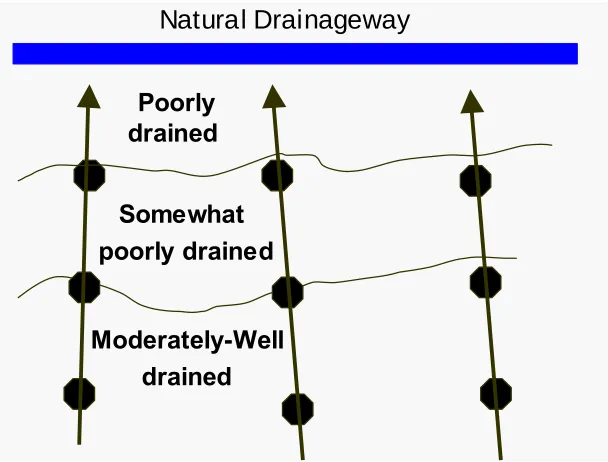
At each site, 2 or 3 transects consisting of 5 to 6 soil plots (well drained moderately well drained, somewhat poorly drained, poorly drained, very poorly drained) were identified for a total of 33 plots. The transects follow a general pattern of well drained to poorly drained positions (Figure 3.2).

Figure 3.2Generalized layout of soil plots (octagons) along transects and their landscape positions. The moderately well drained positions were

highest in elevation, sloping downward though the somewhat-poorly drained plots, toward the lowest point on the local landscape, a natural drainageway.

Each soil plot, (represented by the black octagons in Fig. 3.2), was instrumented with an automated water table monitoring well, and a PVC check well. One transect from each site was instrumented with redox probes, salt bridges, and thermocouples in addition to the wells. One rain gauge per site was located away from the soil plots in an open area.

The hydrodynamics of each soil plot were characterized by a shallow (<2 m) groundwater system raising from the bottom to the surface (endosaturation). Episaturation (perched water table) occurred when the soil below the restrictive layer was unsaturated within 2 m of the surface. Both types of saturation were apparent at the experimental sites.

Moderately-Well drained Somewhat poorly drained

Natural Drainageway

(44)

3.1.1 Richlands Site

General Characteristics

The Richlands site was located in Onslow County, NC, approximately 2.9 km south-southwest of the intersection of State Roads 1230 and 1229, and 320 m west from State Road 1230 (Haw Branch Rd.) at N 34º11’24”, and 77º39’0”. The site was located near or on the Cape Fear/New river drainage divide on a slight ridge within an interstream divide of the Lower Coastal Plain. The soils in the area were permeable and formed in loamy marine sediments. The soil drainage catena consisted of four coarse-loamy, endosaturated soils from moderately-well drained to poorly-drained: Foreston (Coarse-loamy, siliceous, semiactive, thermic Aquic Paleudults), and unnamed transition, referred to as the wet Foreston soil with redox depletions occurring higher in the profile than in the Foreston soil, but lower in the profile than the Stallings (Coarse-loamy, siliceous, semiactive, thermic Aeric Paleaquults) containing a buried spodic horizon occurring at 0.8 m, and Torhunta (Coarse-loamy, siliceous, active, acid, thermic Typic Humaquepts). The upland vegetation was dominated by longleaf pine (Pinus palustris) grading into American Holly (Ilex opaca), greenbrier (smilax, sp.).

There were several drainage features at this site. A 1.8-m deep, 2-m wide road ditch was located about 280 m from the edge of the site and had no apparent effect on the site’s hydrology. Also present on-site was a 1.5-m deep, 3-m wide channelized stream located in a perpendicular fashion in relation to the plots, from 100 to 150 m from the plot lowest on the landscape and 250 meters from the plot highest on the landscape. The road ditch flowed south then flows southwest into the 3-m wide ditch, which had a vertical distance of 0.4 m from the bottom of the stream to the stream bank, eventually draining into the Cape Fear River.

Soil Plots

The site consisted of a total of 12 soil plots, four plots along three transects. Three transects, each containing four plots were oriented in a northwestern to a southeastern