Comparison the Sensitivity Analysis and Conjugate Gradient algorithms for Optimization of Opening and Closing Angles of Valves to Reduce Fuel Consumption in XU7/L3 Engine

(1)

Comparison the Sensitivity Analysis and Conjugate Gradient

algorithms for Optimization of Opening and Closing Angles

of Valves to Reduce Fuel Consumption in XU7/L3 Engine

A. Kakaee1,*, M.Keshavarz2

1_{Assistant Professor,} 2_{BSc. Student, School of Automotive Engineering, Iran University of Science and Technology,} Tehran, Iran

Abstract

In this study it has been tried, to compare results and convergence rate of sensitivity analysis and conjugate gradient algorithms to reduce fuel consumption and increasing engine performance by optimizing the timing of opening and closing valves in XU7/L3 engine. In this study, considering the strength and accuracy of simulation GT-POWER software in researches on the internal combustion engine, this software has been used. In this paper initially all components of engine have been modeled in GT-POWER. Then considering the experimental result, results confirmed the accuracy of the model. After model verification, GT-POWER model with MATLAB-SIMULINK are coupled each other, to control the inputs and the outputs by sensitivity analysis and conjugate gradient algorithms. Then the results compared with experimental results of initial engine too. The results indicated that optimal valve timing significantly reduced brake specific fuel consumption and when is used variable valve system for opening and closing angle of intake and exhaust valves, the mean improvement percentage in brake specific fuel consumption from sensitivity analysis is nearly 5.87 and from conjugate gradient is about 6.69. too, for example with increasing engine speed late closing intake valve causes optimized brake specific fuel consumption and from 3500rpm this trend stops and in 4000rpm and 4500rpm early closing of intake valve results in more optimized brake specific fuel consumption. Then up to 6000rpm again late closing of valve would be favorable. Also results indicated that convergence rate of conjugate gradient algorithm to reaching the optimal point is more than sensitivity analysis algorithm.

Keywords: Sensitivity analysis, Conjugate Gradient, GT-POWER, MATLAB-SIMULINK, valves timing.

1. INTRODUCTION

XU7/L3 engine is the product of Pegout Company whose home production began in 1381 by Iran Khodro Company and now it is the strategic and cheap engine of Iran Khodro which is used in Samand, Pegout 405 and Pars models. The main challenge is high fuel consumption of XU7/L3 engine.

One the most important ways in which the fuel consumption, power and engine performance determines is to calculate the maximum quantity of air during each cycle. So with suitable strategies from the falling the rate of engine volumetric efficiency should be reduced. For this objective, different ways

are suggested, such as enhancing intake and exhaust valve diameter, the increasing the number of input valves to 2 or 3, sketching high performance manifolds, changing software like optimization of intake and exhaust valves timing and optimization of spark timing angle.

As these internal combustion engines are widely used in the world, great research has been done. In these studies beside experimental work different, simulation is used in internal combustion engines.

Shailer during his studies examined experimentally the effects of intake and exhaust valves timing on remaining output gases. In this study he concluded that timing of intake and exhaust valves will have considerable influence on the extent of fuel and fresh air entrance to the combustion chamber. At

Downloaded from www.iust.ac.ir at 20:22 IRST on Friday March 3rd 2017

* Corresponding Author

(2)

144 Comparison the Sensitivity Analysis and Conjugate Gradient…..

the end of exhaust stage and the beginning of inlet stage both intake and exhaust valves simultaneously are open for a short time. As this happens, some outgoing gases can enter internal system through intake valve. Then these outgoing gases enter cylinder again with entering air and fuel which causes pushing back some of the air and reducing volumetric efficiency. This event would have the greatest effect in lower speed of the engine in which the real time when valves are open simultaneously is higher.

Nagao and his colleagues did a wide research on the relation between closing time of intake valve and volumetric efficiency. They realized that in order to get optimized volume efficiency considering loud and speed engine, the time of closing intake valve should be variable.

Asmus have examined the action of intake and exhaust valve in spark ignition engines in his studies. In his study, he pointed to the issue of volumetric efficiency in engines; and considered the timing role of valves the most important factor in optimizing the volumetric efficiency. He also referred to the effect of valve timing on the extent of polluting emissions.

Liguange and his colleagues examined intake and exhaust valve timing effects on spark ignition engines. in this research he examined experimentally the effect of these two factors on power, torque, fuel consumption and the HC polluting materials.

Tottle referred to the process of early or late closing of intake valve controlled engine load compare to basic engine.

Mianzo and his colleagues considered the control of air-fuel ratio in a spark ignition engine with variable valve system, and presented a model with completely variable air-fuel ratio and showed that variable valve system not only changes the air extent entering the cylinder per second but also changes the fuel entering the engine. In this study in the next stage, a linear controller for valve timing has been designed. This controller on the basis of information intake manifold air pressure and air-fuel ratio presents an ideal and proper controller for valve timing to reduce fuel consumption.

Thomas Leroy and his colleagues did a research on controlling intake air path in on engine having variable valve system without EGR. In this study referring to the internal EGR effect in engines having variable valve system and its effects on reducing fuel consumption and emission and also bad effects of increased internal EGR on torque and air-fuel ratio, they presented a new control way by which beneficial effects of variable valve system would be added and bad effects would be reduced. Then suggested strategy have been modeled and tested and their results have been compared to experimental results.

Bin Wu and his colleagues presented optimization valve timing using neural network algorithm. The reason noted for using from this algorithm in this study is was to reduce the time in reaching the optimal point. The engine being used in this study is a gasoline engine with two camshaft having variable valve system and variable valve timing system which have been employed by changing camshaft phase. The result of this study is to reach optimal timing by using neural network in variable valve system engine. Therefore a mathematical model of target engine has been made, then the model was validated by using experimental information and also the constants and performance zone of engine have been realized. To realize these constants in the working zone of engine neural network algorithm have been used. Then to maximize output torque, timing of valves is changed and the best timing in each speed in full throttle condition using neural algorithm is determined. Independent variables in this study are intake and exhaust valve timing, spark timing and air-fuel ratio.

Fontana and his colleagues suggested using the variable valve system and studied it to reduce fuel consumption and improving the performance of low volume engines. Continuously variable valve timing system can optimize fuel consumption and performance of vehicle by making reverse action Miler cycle and considerable EGR.

Variable valve systems also are able to enforce considerable effects on cylinder processes. The most important advantage of variable valve system is known in reducing pumping wastes and reduced mainly fuel consumption has been considered due to this system.

Considering to optimization being very important issue in all sciences and fields, researchers in all sciences have used different kinds of algorithms for optimization. Some examples of using conjugate gradient and sensitivity analysis optimization algorithms that are considered in this study have been brought in previous work.

In year 2000, conjugate gradient algorithm was used to solve finite element equations rigid plastic. The results showed that this algorithm was stable and can be used successfully in solving the problems of metals shaping.

In year 2009, conjugate gradient algorithm was used to calculate single wave problems. Numerical results in this research showed that this algorithm is faster than other numerical methods. Also this algorithm is very strong and it can be easily convergent in all performed examples.

As noted before, up to now only one of these following cases have been generally optimized separately: either intake valve timing or exhaust valve

(3)

A. Kakaee, and M.Keshavarz 145

timing, or opening valves timing or closing valves timing. The case in which all four angles might have been optimized is rarely or never have been done. Also in previous studies neural network algorithm has been used for optimization and the lack of variety in mathematical optimization algorithms is felt in the studies and researches. In this study for the first time XU7/L3 engine is used so that each four opening and closing angles of intake and exhaust valves can be optimized. Also for the first time optimization methods of sensitivity analysis and conjugate gradient which have been used in other activities are used to optimize valves timing.

2. Variable valves system

One the most important ways in which determines the fuel consumption, power and engine performance is calculating the maximum quantity of air during each cycle. So as for as possible, by suitable strategies the fall of volumetric efficiency should be reduced. From presented strategies, in this study improving the volumetric efficiency by optimizing intake and exhaust valve timing was noted, because with the lowest expenses they can achieve acceptable results. Choosing valves optimize timing on the basis of engine speed and engine performance condition and causes optimizing performance level and reducing fuel consumption and emission level. This action results in higher breathing time in faster speed and creates some returning of burnt gases to cylinder (internal EGR) and also solves the torque problem in lower speed and low power in higher speed.

In previous and old engine models valve timing for intake and exhaust was constant, and camshaft was designed according to this timing model. This result in reducing torque in lower speed and lower power in higher speed. To solve this problem variable valve systems were designed. These systems provide suitable timing and lift in different speed.

in higher speed engines naturally engine need more input air, and if opening and closing valve timing are invariable , early closing of intake valve does not allow enough time for air entering the cylinder and results in lower performance. Also in lower speed when the intake valve is open for a longer period, unburnt hydrocarbons exits and causes improper combustion and consequently increases emission output. Variable valves system actually in lower speed provides suitable timing to reduce polluting gases and in higher speed proper timing for increasing engine performance. These two facts

finally results in reducing fuel consumption and improving engine performance in all speeds.

In engines having one camshaft it is not possible to control intake and exhaust valve timing separately because command of opening and closing the intake and exhaust valves is from one camshaft and changing in the camshaft to change timing of a valve influences on the other valve too. For engines having one camshaft which they use variable lift system or variable valve timing with a coupling mechanism is controlled by changing camshaft phase. Although using this system is cheaper and easier than changing the engine to a two camshaft model or removing camshaft and using magnetic valves but it does not have efficiency theirs.

in this study since it is going to optimize all four parameters of opening and closing angle of intake and exhaust valves and considering the facilities of GT-POWER software from technology of removing camshaft and employing magnetic valves has been used.

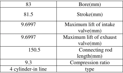
3. Numeral specification of XU7/L3 engine

Numeral specifications of XU7/L3 engine have been brought in following table:

Table 1. numeral specification of XU7/L3 engine

83

Bore(mm)

81.5

Stroke(mm)

9.6997

Maximum lift of intake valve(mm)

9.6997

Maximum lift of exhaust valve(mm)

150.5 Connecting rod length(mm) 9.3

Compression ratio 4 cylinder-in line type

4. XU7/L3 Engine model in GT-POWER software

XU7/L3 Engine model in GT-POWER software is a two dimensional model which different kinds of its input are consist of those related to engine numeral, boundary and initial conditions and some of them are related to performance conditions of engine.

Engine numeral are consist of intake and exhaust manifold maps, combustion chamber map, piston map, crankshaft map of XU7/L3 engine that was obtained from Pegout Company and also engine

(4)

146 Comparison the Sensitivity Analysis and Conjugate Gradient….

performance condition was replaced on the basis of EPCO Company laboratory information. Certain boundary conditions on the basis of gathered information have been replaced. Gasoline used in this model was Iran super gasoline and its information has been received from PETR0 LAB Company.

5. Validation model with experimental result

To validate the model, results have been obtained from engine model and simulation in GT-POWER software from experimental results have been used. To do this, torque and brake specific fuel consumption results compared to experimental results. Available experimental information is on the basis of information achieved from dynamometer of EPCO Company.

As shown in the figure 1, model behavior and experimental information are nearly the same, but in

lower speeds model torque is greater and in higher speeds model torque is smaller. Mean error

percentage between model torque and torque achieved from laboratory is 3.73. according to the curve, it can be seen that in low speeds the model behavior with experimental results, have significant differences. The reason of this error in law speeds is that, the GT-POWER software cannot model some phenomenon such as back flow and RAM effect, although these effects can cause significant reduction in torque and power in low speed. So the torque results of model in low speeds is higher than experimental results, because in the model there are not any reduction in torque due to these effects.

As shown in the figure 2, brake specific fuel consumption in lower speeds is smaller and in higher speed is more than brake specific fuel consumption in laboratory. Mean error percentage between these two is nearly 2.71.

Fig1.validation the torque results of simulation and experimental

Fig2.validation the brake specific fuel consumption results of simulation and experimental

(5)

The difference between data resulted from simulation and experimental is due to this reality that fuel used in simulation has standard specifications, but fuel used in Iran does not have standard specification.

It can be said that results from analysis would have good accuracy.

6. Sensitivity analysis algorithm

In reverse problem the aim is to minimum sum of these squares:       −       −

= m c

T c m E E E E F W

In which, this sum is a function of an unknown parameter P. As an example this unknown parameter in this study is opening and closing angles of intake and exhaust valves, that it is a linear matrix having four columns. So generally the unknown parameter can be shown as follows:

[

]

T

N P P P P r K r r r 2 1 =

In which Pn_{is unknown parameter in nth time} stage and can be shown as follows:

[

]

T

L n n n

n P P P

P ,1 ,2 K ,

r =

In which Pn,l

is unknown parameter lth in nth time stage.

Therefore considering that this parameter changes

the

c

E

_{value, it can consider F as a subordinate of P.} Using derivative in optimized point so that P makes F value optimized the next, equation should be relevant:

0 =       ∂ ∂ P F r

By substituting this condition into equation 1:

0 =       − c m T E E W X

In which X_{is sensitivity matrix:} T T c P E         ∂ ∂ = r X

To optimization it is necessary to regard the c E dependent of P. In case P, it is clear but doesn’t fit in 5 it is necessary to change equal to ∆P. So by using Taylor series and neglecting high degree sentences

the following relation is written for changing c E _: P

E Eck ck

r ∆ + = + X , 1 ,

In which upper case

k

shows repetition and therefore to facilitate computation writing is omitted. By putting 7 in 3 follow equation reached:

So there is an equation to correct P. on the basis of this, the algorithm to solve reverse problem would be as follows.

7. Basic sensitivity analysis algorithm

Reverse problem solving with sensitivity analysis would be as follows:

1-P is estimated.

2-Direct equation is solved and the considered field is determined at proper time.

3-Field values in measurement points,E c _{, is} calculated.

4-F is calculated

5 -sensitivity matrix,X_{, is determined.} 6-equation 8 to reach ∆P is solved. 7-P is corrected

8- Direct equation is solved and the considered field is determined at proper time.

9-Field values in measurement points, E c _{, is} calculated.

10-F is calculated.

11-in case one, the below scales are set, then the answer has been found, otherwise calculation continues from step 5:

1 ε < ∆P r 2 1 ε < − + k k k F F F

In which

ε

1_,ε2_{are small enough values.}

8. Conjugate gradient algorithm

Linear conjugate gradient method in 1950 presented by Hestenes and Stiefel as repetition method to solve linear equations system with positive coefficients matrix. Nonlinear conjugate gradient method is firstly presented by Fletcher and Reeves in 1960. This method is one of the oldest ways to solve long nonlinear optimization. Conjugate gradient method is the same as conjugate directions method which is made by choosing consecutive direction vectors as a conjugate sample of repeated gradients. In this method, because the directions are dependent to gradients, the related process in each stage has a fixed good progress toward the response. Although progress is not very important to a completely second

(6)

order problem, but it is important to none second order problems. So algorithm is presented as follows:

Beginning from every point

x

0_{define as}

0 0

0 g b Qx

d =− = −

and xk+1=xk+αkdk

k T k k T k k Qd d d g − = α

,

dk+1 =−gk+1+βkdk

9. Generalization to nonlinear problems

The general problem of independent minimization that is minimizing f(x), can be solved by presenting suitable approximations from conjugate gradient algorithms. To do this, there are different ways. Choosing the method is to some extent related to some features of f(x) which are easily computable. One of these ways is second order approximation. In this way has been arranged the following parameters

in

x

k_:

)

(

,

)

(

_k T _k

k

f

x

Q

f

x

g

↔

∇

↔

And by using them so that they are calculated again in each stage all necessary values to present main conjugate gradients algorithm are computed.

Conjugate gradient methods are used for none second order problems when they are not usually ended in n stages. Therefore can easily finding the new directions on the basis of algorithms continued and stop it when a stopping scale provided. Because conjugating direction vectors in pure algorithm of conjugate gradient is dependent of choosing negative gradients as first direction, it seems that the method of starting again would be preferred more; thereafter always this method is used. So total algorithm of conjugate gradient is presented as follows:

By starting point

x

0_{is computed}

T

x

f

g

₀

=

∇

(

₀

)

and is replaced

d

0

=

−

g

0

For

k

=

0 ,

1 ,...,

n

−

1

T k

k

f

x

g

₊₁

↔

∇

(

₊₁

)

is computed

3- Is replaced

x

0_with

x

n_{and get back to stage}

1.

An interesting feature of this algorithm is that any linear search in any stage as Newton pure alternative isn’t needed. Besides the algorithm for second order problems for a few stages becomes convergent. Bad features of this algorithm are the fact that

f

(

x

_k

)

should be calculated in any point which is often impractical, and that this algorithm in this form isn’t globally convergent.

It is not possible to use

Q

↔

f

(

x

k

)

_directly.

Firstly instead of using

α

k_{formula in stage (2-a)}

α

k

is reached at a linear search that minimizes the target function. This is compatible with second order

formula. Secondly

β

k_{formula in stage 2-c is}

replaced by another formula so that in any case it is equivalent to (2-c) second order position.

The first suggested way of this kind was Fletcher-Reeves method as follows:

T k k k T k k g g g g +₁ +₁ =

β

Complete algorithm using method of starting again is as stated below:

By starting point

x

0_{is computed}g0=∇f(x0)T_and

is replaced

d

0

=

−

g

0

For

k

=

0 ,

1 ,...,

n

−

1

b)

T k

k

f

x

g

₊₁

↔

∇

(

₊₁

)

is computed

Except

k

=

n

−

1

, is replaced dk+1=−gk+1+βkdk in which k T k k T k k g g g g +1 +1 =

β

Is replaced

x

0_with

x

n_{and get back to stage 1.}

One another way of this kind is Polak-Ribiere in which k T k k T k k k g g g g

g ₁ ) ₁

( ₊ − ₊ = β k T k k T k k Qd d Qd g ₊₁ − =

β

In which:

g

k

=

Qx

0

−

b

Is replaced xk+1=xk+αkdk_{in which} k T k k T k k

Qd

d

g

−

=

α

Except

k

=

n

−

1

, is replaced dk+1=−gk+1+βkdk

in which k k

T k k k T k k d x f d d x f g ) ( ) ( 1 + = β

a) Is replaced xk+1=xk+αkdk_{in which}

α

k

minimizes

f

(

x

k

+

α

k

d

k

)

(7)

Experimental results that show Polak-Ribiere method is better than others methods all of this general kind.

10.Coupled model of GT-POWER And MATLAB-SIMULINK

Considering the noted issues optimization is on the basis of model sensitivity extent to input changes. The provided model on the basis of output sensitivity extent compare to inputs tries to get the nearest point to the target function. Here the input parameters are opening and closing timing of intake and exhaust valves and output parameter is brake specific fuel consumption. In order to control inputs and output of the model, two software are coupled. So in this way the basis of output related to GT-POWER model, the software MATLAB-SIMULINK On the basis of

sensitivity analysis and conjugate gradient algorithms gets suitable inputs to get a model with the least error.

11.Optimization of brake specific fuel consumption by changing the valves timing

In this chapter with coupled of GT-POWER and MATLAB-SIMULINK by using sensitivity analysis and conjugate gradient algorithms to optimize the opening and closing angles of valves to minimize brake specific fuel consumption. Also the results are compared to related basic engine in order to examine their effect on reducing fuel consumption.

In figure 4 results of brake specific fuel consumption versus engine speed in three modes of using sensitivity analysis algorithm, using conjugate gradient algorithm and the mode in which variable valve system is not used have been presented.

Fig3.: Coupled model of GT-POWER And MATLAB-SIMULINK

Fig4.Changes of BSFC versus engine speed in three using conditions from sensitivity analysis algorithm, conjugate gradient algorithm and without variable valve system

(8)

Fig5.Changes of torque versus engine speed in three using conditions from sensitivity analysis algorithm, conjugate gradient algorithm and without variable valve system

As shown in the figure 4, in diagram using variable valve system, brake specific fuel consumption in all speeds is reduced, and this reduction is especially considerable in high speeds. Also it is saw that both optimization algorithms have very close answer to brake specific fuel consumption. From 3000rpm downward the answers of both algorithms are exactly equal and higher than 3000rpm the answers have very little difference. With doing necessary calculations in optimized state is saw that when variable valve system for opening and closing angle of intake and exhaust valves is used, the mean improvement percentage in brake specific fuel consumption from sensitivity analysis is nearly 5.87 and from conjugate gradient is about 6.69.

In figure 5, torque results versus engine speed in three using conditions from sensitivity analysis algorithm, conjugate gradient algorithm and without variable valve system have been brough

As shown in the figure 5, by using variable valve system, torque will increase in all speeds. Also it is saw that when variable valve system for opening and closing angle of intake and exhaust valves is used, the mean improvement percentage in torque from sensitivity analysis is nearly 5.07 and from conjugate gradient is about 6.18.

Also results related to the number of convergent steps of both algorithms with equal initial condition in every speed have been brought in table 2. The results from this table show that the convergent speed of conjugate gradient algorithm in reaching to optimized point is much higher than sensitivity analysis. This results from the point that conjugate gradient algorithm uses suitable directions in reaching to the answer.

Table.2.Results related to the number of convergent steps of both

algorithms with equal initial condition in every speed

Number of steps- sensitivity

analysis Number of

steps- conjugate

gradient Engine

speed(RPM)

19 4

1500

31 7

2000

17 11

2500

28 6

3000

20 15

3500

16 14

4000

15 5

4500

19 20

5000

18 17

5500

24 19

6000

12.Optimized valve timing

After calculations, optimized opening and closing valve timing for the two algorithms has been drawn in each speed in the following diagrams.

As shown in the figure 6, by increasing engine speed to 3500rpm early opening of intake valve causes optimized brake specific fuel consumption, and from 3500rpm this trend changes and in 4000rpm with late opening of intake valve causes optimized brake specific fuel consumption, then up to 6000rpm again early opening of intake valve would be favorable for optimized brake specific fuel consumption. The fact that this carve has a minimum in 3500rpm can explain as follow; although with increasing engine speed and early opening the intake

(9)

valve, the greater air volume would enter the cylinder and it causes the BSFC reduction, but on the other hand, early opening of intake valve causes more burnt gases volume enters the new cycle and results in incomplete combustion and finally increases the BSFC. The effects of these factors are responsible that curve has a local minimum.

Also it is seen that both algorithms except in 1500rpm and 6000rpm would have the same answer.

As shown in the figure 7, by increasing engine speed, late closing intake valve causes the optimized brake specific fuel consumption and from 3500rpm this trend stops a little and in 4000rpm and 4500rpm early closing of intake valve results in more optimized brake specific fuel consumption .then, up

to 6000rpm again late closing of valve would be favorable. Also these two algorithms except for 3500rpm and 4000rpm have the same result. The fact that this carve has local maximum local minimum in 3500rpm and 4500rpm can explain as follow; although with increasing engine speed and late closing the intake valve, the greater air volume would enter the cylinder and it causes the BSFC reduction, but on the other hand, late closing of intake valve (it’s more opening in compression process) causes an amount of entrance air to the cylinder come back to the intake manifold and finally increases the BSFC. The effects of these factors are responsible that curve has local maximum and minimum.

Fig6.Changes of angle for opening intake valve versus engine speed from sensitivity analysis and conjugate gradient algorithms with target of optimized BSFC

Fig7.Changes of angle for closing intake valve versus engine speed from sensitivity analysis and conjugate gradient algorithms with target of optimized BSFC

(10)

Fig8.Changes of BSFC versus closing angle of intake valve in 3500rpm

Fig9.: Changes of angle for opening exhaust valve versus engine speed from sensitivity analysis and conjugate gradient algorithms with target of optimized BSFC

It is seen that the answers for closing angle of intake valve in 3500rpm from both algorithms have great difference, regardless of this fact, brake specific fuel consumption in this speed will have nearly the same result. In figure 8 when other angles are fixed, the diagram for brake specific fuel consumption by changing the closing angle of intake valve in 3500rpm has been drawn. As it is seen in this diagram it has two local minimum so that each algorithm is convergent with one of them, and as it is expected, brake specific fuel consumption of these two points are very close to each other.

As shown in the figure 9, by increasing speed up to 2500rpm, early opening of exhaust valve results in optimized brake specific fuel consumption and in 2500rpm this trend stops and up to 3500rpm, late opening of exhaust valve results in optimized brake specific fuel consumption, then from 4000rpm, again, early opening of exhaust valve results in optimized

brake specific fuel consumption. After that, up to 6000rpm late opening exhaust valve would be desirable.

By increasing engine speed, with early opening of exhaust valve, more volume of burnt gasses guided to the out of cylinder and results in volumetric efficiency increasing and BSFC reduction. But if, with increasing engine speed, this early opening continues, it results to not using all the piston work in the expansion process which causes the BSFC increasing. The effect of these two factors causes the curve to have an increasing or decreasing trend according to the engine speed.

It is seen differences between results from two algorithms for this angle are relatively great comparing to other angles, regardless of this fact brake specific fuel consumption in this speed will have nearly the same result. In figure 10, the diagram for brake specific fuel consumption by changing the

(11)

opening angle of exhaust valve in 2500rpm while other angles are fixed has been drawn. As seen this diagram in minimum point has little sensitivity to changes in opening angle of exhaust valve that is in minimum point the diagram is smooth and every algorithm is convergent to some place of this diagram smoothness.

As shown in the figure 11, by increasing speed late closing of exhaust valve results in optimized brake specific fuel consumption and from 4500rpm this trend stops a little and in 5000rpm and 5500rpm early closing of exhaust valve causes a more optimized brake specific fuel consumption. Then in 6000rpm again late closing of exhaust valve would be desirable. By increasing engine speed, with late closing of exhaust valve, more volume of burnt gasses guided to the out of cylinder and results in volumetric efficiency increasing and BSFC reduction. But if, with increasing the engine speed, late closing also continues, it results in an amount of entrance air to the cylinder come back to the exhaust manifold during the new intake process, and it results the BSFC reduction.

It can be seen that the results of two algorithm for this angle, is too similar, but in other angles, the differences of two algorithm is very high. The reason is that the effective parameters in optimizing BSFC, are the opening and closing angles of intake valve and opening angle of exhaust valve and the effect of this angle on optimization variable is low, so two algorithms for this angle, have almost similar results.

To explain the reason for upper results, it should be said that calculating the maximum air volume in cylinder in each cycle results increased volumetric efficiency and therefore reduced brake specific fuel consumption. So if timing of opening and closing of valves is away, that would increases the air volume in cylinder in each cycle then fuel consumption falls down. So by increasing engine speed because piston speed increases if intake valve opens earlier and closes late, air that inter to cylinder increases during each cycle and brake specific fuel consumption decrease. With the same reason increase in engine speed if exhaust valve opens earlier and closes later, burnt gases in the cylinder of the previous cycle gets out better and air that inter to cylinder increases therefore brake specific fuel consumption reduces

Big gaps which sometimes are seen in valves timing, it is explained in this way. Results of brake specific fuel consumption depends on engine power and fuel consumption, for this reason in some engine speeds, changes in power and fuel consumption are in the opposite direction and cause big gaps between two sequent timings. Also in some engine speeds, valve timing for brake specific fuel consumption will follow a nearly fixed trend. To explain this it can be said that both power and fuel consumption will follow a decreasing trend or will get an increase similar to valve timing change, and brake specific fuel consumption will nearly remain unchanged.

Fig10. : Changes of BSFC versus opening angle of exhaust valve in 2500rpm

(12)

Fig11. Changes of angle for opening exhaust valve versus engine speed from sensitivity analysis and conjugate gradient algorithms with target of optimized BSFC

13.Results

In this paper sensitivity analysis and conjugate gradient algorithms presented and these are compared for optimizing the controls parameters such as valves timing with target optimized brake specific fuel consumption. In this study, considering the strength and accuracy of simulation GT-POWER software in researches on the internal combustion engine, this software has been used. In this paper initially all components of engine have been modeled in GT-POWER. Then considering the experimental result, results confirmed the accuracy of the model. Mean error percentage between model torque and torque achieved from laboratory is 3.73. Mean error percentage between model brake specific fuel consumption and brake specific fuel consumption achieved from laboratory is nearly 2.71. After model verification, GTPOWER model with MATLAB -SIMULINK are coupled each other to control the inputs and the outputs by sensitivity analysis and conjugate gradient algorithms. After computations, below results achieved:

1- With optimizing change of valves timing in spark ignition engines their performance and brake specific fuel consumption in all speeds would increase. With doing necessary calculations in optimized state, is saw that when variable valve system for opening and closing angle of intake and exhaust valves is used, the mean improvement percentage in brake specific fuel consumption from sensitivity analysis is nearly 5.87 and from conjugate gradient is about 6.69.

2- The convergent speed of conjugate gradient algorithm to reaching the optimized point is much

higher than sensitivity analysis. This results from the point that conjugate gradient algorithm uses suitable directions to reaching the answer.

3- By increasing engine speed to 3500rpm, early opening of intake valve causes, optimized BSFC, and from 3500rpm this trend changes and in 4000rpm with late opening of intake valve causes optimized BSFC, then up to 6000rpm again early opening of intake valve would be favorable for optimized BSFC. Also it is seen that both algorithms except in 1500rpm and 6000rpm would have the same answer.

4- By increasing engine speed with late closing intake valve, causes optimized BSFC and from 3500rpm this trend stops a little and in 4000rpm and 4500rpm early closing of intake valve results in more optimized BSFC .then, up to 6000rpm again late closing of valve would be favorable. Also these two algorithms except for 3500rpm and 4000rpm have the same result.

5- By increasing speed up to 2500rpm, early opening of exhaust valve results in optimized BSFC and in 2500rpm, this trend stops and up to 3500rpm, late opening of exhaust valve results in optimized BSFC, then from 4000rpm again early opening of exhaust valve results in optimized BSFC. After that, up to 6000rpm late opening exhaust valve would be desirable.

6- By increasing speed, late closing of exhaust valve, results in optimized BSFC and from 4500rpm this trend stops a little, and in 5000rpm and 5500rpm, early closing of exhaust valve causes a more optimized BSFC. Then in 6000rpm again,

late closing of exhaust valve would be desirable.

References

(13)

[1]. Mehdi.Keshavarz, Optimization Of Opening And Closing Angles Of Inlet And Exhaust Valves For Reduction of Fuel Consumption And Emission of XU7/L3 Engine, A Thesis Submitted in Partial Fulfillment of the Requirement for the Degree of Master of Science in Automotive Engineering, November 2011

[2]. John B. Heywood."Internal combustion engine fundamentals" McGraw-Hill Inc, 1998.

[3]. Paul J.Shayler, "experimental investigations of intake and exhaust valve timing effects on charge dilution by residuals,fuel consumption and emissions", SAE world congress and exhibition, Aprill 2007.

[4]. Nagao.F. , Nishiwaki.K. , Yokoyama.F. ; "Relation between Inlet Valve Closing Angle and Volumetric Efficiency of a Four Stroke Engine" Bulletin of JSME, vol. 12, p.p. 894-901, 1969.

[5]. Asmus.T.W , Corp.C. ; "Valve Events and The Engine Operation" SAE, No.820749. 1982 [6]. Liguang Li , Yan Su,Yunkai Wang , " effects of

intake valve closing timing on gasoline engine performance and emissions " , SAE international fall fuels and lubricants meeting and exhibition, San Antonio, TX, USA. September 2001.

[7]. J.H.Tuttle "controlling engine load by means of early intake valve closing" , SAE paper, No.820408

[8]. Mianzo.L. , Peng.H. ; "Modeling and Control of Variable Valve Engine, Variable Valve Actuation" American control conference Chicago,2000

[9]. Thomas Leroy , JonathanChauvin , NicolasPetit , "Motion planning for experimental air path control of a variable-valve-timing spark ignition engine " Control Enginering Practice , Elsevier journal, 2008

[10].Wu.B. Prucka.R.G. Filipi.Z.S. Kramer.D.M. Ohl.G.L. ; "Cam-Phasing Optimization Using Artificial Neural Network as Surrogate Models-Maximizing Torque Output" SAE paper, No.01-3757. 2005

[11].Fontana.G. , Galloni.E. , "Variable valve timing for fuel economy improvement in a small spark-ignition engine" Applied Energy, Elsevier journal, vol. 86, pp. 96-105, 2009

[12].Z.Y. Jiang, W.P. Hu, P.F. Thomson, Y.C. Lam""Solution of the equations of rigid-plastic FE analysis by shifted incomplete Cholesky factorisation and the conjugate gradient method in metal forming processes"" Journal of

Materials Processing Technology vol.102 ,pp.70-77 , 2000.

[13].Jianke Yang "" Newton-conjugate-gradient methods for solitary wave computation ""Journal of Computational Physics ,vol.228 , pp 7007–7024 , 2009

[14].David.G.Luenberger."linear and nonlinear programming"Addision-Wesley,1984.