Manufacturing Cycle Time Analysis and Scheduling to Optimize Its Duration

0 INTRODUCTION AND PREVIOUS INVESTIGATIONS

Inherent to the investigation of the manufacturing cycle time is a set of activities, from defining the optimum production lot, calculations of the quantity of required parts, production preparation and launching, cycle scheduling, management of production activities with current asset engagement, to the analysis and investigations of material flow.

Systems for the production of weaponry and military equipment (special-purpose products) have specific positions and roles. Production is regulated by special legal provisions, whereby business operations, among other things, are determined by the product choice and quality, manufacturing, financial and human resources, serial production, complex and diverse technologies, short-term deliveries (as a rule), demands for modification of standard product versions, possibilities to supply specific materials and parts, high-level security during the production, handling, storage and utilization of means.

The start-to-finish treatment cycle implies the choice of benchmark points within which time flows. In terms of production management, the manufacturing cycle determines the duration of business and production activities needed to carry out the overall manufacturing process of a certain quantity of product with minimum time flow, maximum utilization of manufacturing capacity and optimal engagement of financial resources.

Production planning and management is a complex set of activities, as confirmed by many

works dealing with this problem [1] to [2]. Eckert and Clarkson [3] describe current planning practice in the development processes for complex industrial products and the challenges associated with it, making suggestions for its improvement. Since they view planning as a project, they emphasize that in order to reduce the duration of project the overlap between tasks must be optimized. In contrast, Alfieri et al. [4] observe the manufacturing-to-order system producing complex items as a set of activities whereby a project scheduling approach should be applied to production planning. They have developed two mathematical models for the execution of activities, i.e. their overlap with a smaller number of activities (up to 30 and up to 60 respectively). Dossenbach [5] analyses the possibility of reducing manufacturing cycle times in the wood-processing industry.

In his work [6], Johnson provides a framework for reducing manufacturing throughput time. It is based on identifying the factors that affect manufacturing throughput time, the actions that can be taken to diminish their impact, and their interactions. The framework is sufficiently detailed to provide guidance to the industry practitioner on how to reduce throughput time, but is sufficiently general to be applied in most manufacturing situations.

Lati and Gilad [7] have developed an algorithm for reducing losses in the semiconductor industry, called the MinBIT (minimizing bottleneck idle time) algorithm, which represents a new method for sequencing the handler’s moves; the authors also highlight its application in other industries to bring

Manufacturing Cycle Time Analysis and

Scheduling

to Optimize Its Duration

Jovanovic, J.R. – Milanovic, D.D. – Djukic, R.D.

Jelena R. Jovanovic 1,2,3,* _{– Dragan D. Milanovic}2 _{– Radisav D. Djukic}1,3 1 _{Technical College of Applied Studies, Cacak, Serbia}

2 _{University of Belgrade, Faculty of Mechanical Engineering, Serbia} 3 _{‘Sloboda’ Company, Serbia}

This paper reports the results of investigations on manufacturing cycle times for special-purpose products. The company performs serial production characterized by complex and diverse technologies, alternative solutions and combined modes of workpiece movement in the manufacturing process. Because of various approaches to this problem, an analysis of previous investigations has been carried out, and a theoretical base is provided for the technological cycle and factors affecting the manufacturing cycle time. The technological and production documentation of the company has been analysed to establish the technological and real manufacturing cycle times, total losses and flow coefficients. This paper describes the original approach to production cycle scheduling on the grounds of investigations of manufacturing capacity utilization levels and causes of loss, in order to measure their effects and to reduce the flow coefficient to an optimum level. The results are a segment of complex studies on the production cycle management of complex products, accomplished in the company in the period from 2010 to 2012.

about cycle time reductions and throughput increases. Hermann and Chincholkar [8] describe a decision support tool that can help a product development team to reduce manufacturing cycle time as early as in the product design phase. The design for production (DFP) tool determines how manufacturing a new product design affects the performance of the manufacturing system, taking into account the capacities available and estimating the manufacturing cycle time.

Bottleneck control in real time production [9], prioritizing machine fleet preventive maintenance [10], spare parts inventory for maintenance, optimization of initial buffer adjustment [11], reduction of machine setup time [12] and predicting order lead times [13], can lead to production effects improvement and manufacturing cycle time reduction.

Ko et al. [14] investigate the possibility of reducing cycle times in mass production by input and service rate smoothing.

Based on the analysis of cited works, the following can be concluded:

• A generally accepted approach is to use the flow coefficient as a measure of the manufacturing process efficiency, which rests upon the comparison between the accomplished and technological (ideal) values of the manufacturing cycle.

• Investigations most commonly focus on the cycle within the framework of one-off and small-scale production, where technological values are determined in terms of the consecutive mode of workpiece movement and large-scale and mass production, and where technological values are determined in terms of parallel moves (analysis involves takt time and technological line productivity).

• The technological cycle duration, under conditions of serial production characterized by discontinuity, is calculated using the formulas for the consecutive or parallel mode of workpiece move, depending on the size of the production lot and the author’s assessments.

In terms of theoretical considerations and industrial practice, it is of crucial importance to master the key parameters that affect the manufacturing cycle duration under the conditions of complex-product serial production with dominating interruptible processes conditioned by complex and diverse technologies. The manufacturing process includes highly productive machines, having standard and specialized applications, with high concentrations of technological operations, but also the universal-type equipment with expressed differentiation of

operations. The technological procedure embraces both productive and non-productive operations with the involvement of technologies used to change the workpiece shape and features.

All the aforementioned manufacturing conditions require an integrated approach in investigating the manufacturing cycle that should enable its permanent reduction through dynamic and cyclic process oriented to:

• generating an exact theoretical framework for calculating the technological cycle duration based on a combined mode of organizing the sequence of technological operations,

• identifying the causes of losses, measuring their effects on manufacturing capacity utilization level and cycle duration,

• manufacturing cycle design with scheduled losses that are lower than planned, taking into account the optimal overlap of activities, and

• production launching, analysing and measuring the manufacturing process efficiency based on a comparison of real and designed values.

Based on all the above-mentioned factors, it can be inferred that cycle time duration is a stochastic quantity directly affected by:

1. factors related to product development and production program (e.g. total number, types, quantities and product complexity),

2. manufacturing capacity of the system and manufacturing process automotive level (e.g. human resources, equipment, space),

3. financial potentials (e.g. current assets, input inventories, size and structure of unfinished production),

4. technologies applied and manufacturing equipment layout (e.g. workplaces),

5. volume of production and modes of workpiece move in the manufacturing process (e.g. optimum production lot, type of production),

6. factors related to the adopted principles of manufacturing and informatics support in all material flow phases,

7. methods applied in production planning, monitoring and management, and

8. causes of cycle losses.

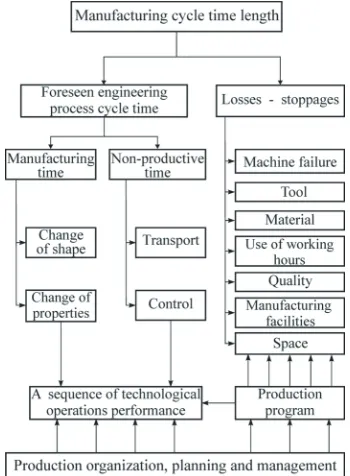
non-productive time involves operations related to transport and control.

Fig. 1. Several factors on manufacturing cycle time duration The exposition of the investigation results will be organized into three sections treating:

• Theoretical and technological bases for technological (ideal) manufacturing cycle time scheduling, depending on the mode of organizing the sequence of operations, with investigation results.

• Investigation of real manufacturing cycle time duration, manufacturing capacity utilization level (machines, human resources in manufacturing) and causes of losses.

• Manufacturing cycle scheduling of a chosen product, production launching according to the designed model and investigations of the flow coefficient K based on a comparison of realized and designed states in the production process (Kp), i.e. in terms of comparisons between real and technological (ideal) cycles (Kt) calculated using formulas for combined modes of workpiece movements.

1 TECHNOLOGICAL (IDEAL) MANUFACTURING CYCLE

The production program of the plant P, Eq. (1), consists of products Xj and parts xi. The process of parts manufacturing is defined by a set of data A

composed of the number of technological operations

n, ordered set θn of times per operation ti and lot size

q, Eq. (2). Technological manufacturing cycle Tt , which is also an ideal cycle Tci, Eq. (3), includes the time needed for performing all n operations predicted by the technological procedure, on the products of a single lot. Production organization plays a critical role in determining the technological cycle, in which moves may be consecutive Tt(u) (Eq. (4)), parallel

Tt(p) (Eq. (5)) and combined Tt(k) (Eqs. (6) or (7)), depending on the type of production, consist of a complex set of features.

P=

{

(

)

}

x A_i: =

{

}

{

}

T Tt = ci=

{

}

T q t

H x i m P A n q

tu i i n i n ( )_{= , , , , ,} ⋅ ∀ =

(

)

{

}

∑

1 _{1 θ (4)}

T t q t

H t t i n

x i m P A

t p i i n i i

( ) max

max

, max , ,

, = +

(

)

{

}

(

)

∑

1 1 ₁

1 ==

{

}

T

t q t t

H

t t t k n

tk i i

n

k

k j j

k k k

( ) _, , = +

(

)

< ≥ ∀ =

(

)

∑

∑ ∑

1 tt t t j n

x i m P A n q

j j j

i n

− ≥ < +∀ = −

(

)

∀ =

(

)

{

}

1 1 2 1

1

, ,

, , , ,θ (6)

T t q t t F

H

t t F t t

tk i i

n

i i i

i n

i i i i i

( ) = = −

− −

=

+

(

)

(

)

> ⇒ = ∧ ≤

∑

∑

1 1 1

1

1

1

,

11 0 0 0

1

⇒ = ∧ =

∀ =

(

)

{

}

F t

x i m P A n q

i

i n

,

, , , .θ (7)

Depending on the time units in which the cycle time duration is expressed, the values of parameter H

are determined by Eqs. (8) to (11).

H = 1 → Tt[norm hours/lot], (8)

H = CS → Tt[shift/lot], (9)

H = CS·Sd → Tt[workdays/lot], (10)

H C S D

D T

s d k

r t

= ⋅ ⋅1 = →

[

]

where:

ti total time per technological operation in norm hour/piece,

Cs effective working hours in a shift,

Sd number of shifts per day,

Dk total number of calendar days in a corresponding period of time,

Dr total number of workdays in a corresponding period of time,

tmax run-time length of the longest technological operation,

tk , tjtechnological operations that satisfy the condition from Eq. (6),

Fi a constant that takes the value of 1 or 0,

δ calendar and workdays ratio.

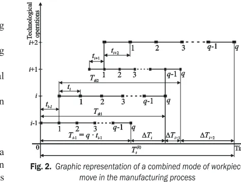
The combined type of work flow in a manufacturing process is most often encountered in serial production. Its goal is to eliminate downtimes

emerging at some workplaces (operations) of a parallel type due to the different durations of successive operations, Fig. 2.

Fig. 2. Graphic representation of a combined mode of workpiece move in the manufacturing process

Table 1. Sequence of technological operations with norms and technological cycle values for a job order lot of q = 30,000 pieces, in calendar days

Order of _operation Machine code

Capacity in a shift q_Si [piece/shift]

Time per operation

ti

[cmh/piece]

Parameters for technological cycle calculations

tmax tk tj Fi (ti– ti–1) · Fi

1 2 3 4 5 6 7 8 9

1 - 125000 6 - - - 1 6

2 M1 18750 40 - 40 - 1 34

3 - 93750 8 - - 8 0

-4 M2 5600 134 - 134 - 1 126

5 - 93750 8 - - 8 0

-6 M1 18750 40 - 40 - 1 32

7 - 93750 8 - - 8 0

-8 M3 4300 172 - 172 - 1 164

9 - 93750 8 - - 8 0

-10 M4 18750 40 - 40 - 1 32

11 - 93750 8 - - 8 0

-12 M5 4300 172 - 172 - 1 164

13 M6 4300 172 - - 172 0

-14 M7 2500 300 300 300 - 1 128

15 - 93750 8 - - 8 0

-16 - 15000 50 - - - 1 42

17 - 8200 92 - 92 - 1 42

18 M8 18750 40 - - 40 0

-19 - 8200 92 - 92 - 1 52

20 M9 25000 30 - - 30 0

-21 - 8200 92 - 92 - 1 62

22 - 375000 2 - - - 0

-Σ 1522 - 1174 290 - 884

H C S Dk

Dr s d

= ⋅ ⋅ =1 7 5 1 3 0 704 6 866⋅ ⋅ = = =365=

257 1 42

δ . . . . , δ . ,

1.1 Calculations of Technological Cycle for an Analysed Product

The analysed product is manufactured in three displaced organizational units: 1120, 1170 and 1630. The manufacturing process engages nine different machines (M1 to M9). Ten types of technology are applied, arranged into four groups: heat treatment (one type of technology), mechanical processing/ deformation, cutting (five types of technologies), chemical preparation (two types of technologies) and surface finish (two types of technologies). Of 22 technological operations, 17 are manufacturing (six operations are related to change in shape, 11 to change of characteristics) and five operations are non-manufacturing (four operations refer to control, one to transport). The total time needed to produce a single part amounts to 0.017 norm hours. The norm structure is composed of 20% machine time (only a machine is operating), 59% combined time (both a handler and a machine are operating simultaneously) and 21% manual time (only handlers are engaged).

On the grounds of technological procedure and Eqs. (4) to (11) for a job order lot of 30,000 parts, Table 1 shows data needed for calculations of the technological cycle as well as the cycle values for consecutive, parallel and combined modes of workpiece movement, Eq. (12). Technological cycle

Tt(k) is 2.95 times longer than Tt(p) and by 1.72 times shorter than Tt(u), respectively.

The obtained results confirm the correctness of the approach in which the flow coefficient Kt is defined as a real to technological Tt(k) ratio instead of

Tt(u) or Tt(p) as has been the practice to date.

Tt( )p ≅14<Tt( )k ≅39<Tt( )u ≅67. (12)

2 ANALYSIS OF CYCLE TIME AND CAUSES OF LOSSES IN MANUFACTURING CAPACITY

Technological cycle Tt is an ideal manufacturing cycle

Tci because the corresponding Eqs. (4) to (11) do not include losses in the cycle that are unavoidable in the manufacturing process. Unlike technological, cycle time, real duration Tcs includes all generated losses

Gcs. Methods for data collecting on manufacturing cycle time duration Tcs can be arranged into three groups.

The first group of methods is based on the analysis of manufacturing, planning and other documentation for the system, when it is possible to establish the start and end dates for the manufacturing

process. The most commonly used manufacturing documentation items are job order documents (term cards, material requisition, worksheets, delivery notes, etc.), documents of technical control and various reports on the current state of the manufacturing process. For the processes that are rarely repeated, e.g. performed once a year or once in six months, planning documentation and other documents are used, relating to supply, reception, storage and sales for the approximate definition of benchmark points.

The second group of methods includes those based on the measurement of cycle time duration and its components. The chrono-metering method is applied for shorter cycle time durations, while the method of current observations is used for longer cycle time durations that are frequently repeated. Cycle time duration is measured on a representative sample of parts.

The third group is based on estimating the total duration of cycle times. These methods are applied for cases in which the above methods are not applicable or require much effort.

2.1 Real Cycle, Losses in the Cycle and Flow Coefficient

The analysis of manufacturing documentation (term cards and reports on the current state of the manufacturing process) was used to determine cycle time duration Tcs for a chosen part based on data about the realized start and end dates of production.

Total losses in the cycle Gcs are calculated with the help of Eq. (13) when the technological cycle duration Tt is subtracted from the real cycle time duration, paying attention to the type of production. Total losses consist of intra-operational Guo and inter-operational Gmo losses.

Since the company practices a serial type of production, the total losses in the cycle Gcs, average losses per operation ε and flow coefficient

Kt, representing the correlation between real and technological cycle time duration, will be calculated using Eqs. (14) to (16). Various approaches to determining the correlation between real and theoretical cycle time duration can be also found in papers [15] and [16].

G_cs=T_cs− =T G_{t uo}+G_mo, (13)

Gcs=Tcs−Tt( )k, (14)

ε =G

K T T t cs

tk

= _{( )}. (16)

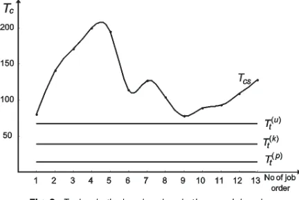
After the cycle time analysis has been completed, the results are presented in Table 2 and Figs. 3 and 4. A total of 13 job orders, seven in 2010 and six in 2011 for the quantity of 30,000 pieces each year were analysed.

Fig. 3. Technological and real cycle time per job order Flow coefficient Kt (Fig. 4) takes values within 2.02 to 5.18 range. Total losses in the cycle (Gcs) measured against the technological value Tt(k) range from 39.4 to 161.4 calendar days, and losses are higher, on average, by 2.24 times than technological cycle duration. Taking into account the parameters from Eq. (17) and the fact that this is a serial repeating

production, it can be inferred that the production planning and management process is uncontrollable, experience-based, lacking identified and quantified causes of losses in the cycle.

T T

G K

tk cs

cs t

( ) _{. , , . . ,}

. . , . .

= ≤ ≤ ≤ ≤

≤ ≤ ≤ ≤

38 62 78 200 1 8 7 3

39 4 161 4 2 02 5

ε

118. (17)

Fig. 4. Flow coefficient Kt per job order

2.2 Utilization of Machine Capacity and Structure of Losses per Cause of Downtime

Taking into account the obtained results, Eq. (17), and the importance of the analysed product that is on a critical path of the manufacturing cycle of four complex products making up the framework of the 2010 and 2011 production programs, the causes and

Table 2. Real manufacturing cycle time duration Tcs, total losses in the cycle Gcs, losses in the cycle per operation ε and values of flow coefficient Kt, in calendar days

No

Job order (JO) Cycle time duration Losses Flow

coefficient

Kt

Lot Quantity Manufacturing date T_t(k) _{Tcs Gcs} ε

Start End

1 2 3 4 5 6 7 8 = 7–6 9 10=7/6

1 04/10 30000 30.08.2010 17.11.2010

38.62

80 41.4 1.9 2.07

2 05/10 30000 30.08.2010 17.01.2011 141 102.4 4.7 3.65

3 06/10 30000 30.08.2010 16.02.2011 171 132.4 6.0 4.43

4 07/10 30000 30.08.2010 17.03.2011 200 161.4 7.3 5.18

5 08/10 30000 18.09.2010 31.03.2011 195 156.4 7.1 5.05

6 09/10 30000 16.12.2010 08.04.2011 114 75.4 3.4 2.95

7 10/10 30000 16.12.2010 21.04.2011 127 88.4 4.0 3.29

8 01/11 30000 23.02.2011 06.06.2011 104 65.4 3.0 2.69

9 03/11 30000 09.04.2011 25.06.2011 78 39.4 1.8 2.02

10 04/11 30000 09.04.2011 06.07.2011 89 50.4 2.3 2.30

11 05/11 30000 07.07.2011 07.10.2011 93 54.4 2.5 2.41

12 06/11 30000 07.07.2011 23.10.2011 109 70.4 3.2 2.82

13 07/11 30000 08.09.2011 13.01.2012 128 89.4 4.1 3.31

measurements of losses were investigated with regard to the manufacturing capacity. The causes of losses (i) were identified (Eq. (18)), and machine capacity utilization level ηm was established for the operations with machines and combined time cycles (Eq. (19)), with respect to cycle times in the structure of norm-hour per technological operation. Machine capacity utilization level and current losses, per downtime cause, can be measured with different techniques [17].

g_m g_i i K A M C I V O X i

= =

{

}

=

∑

1 8

, , , , , , , , , (18)

η_m n _i i

n g

n n

= ( ) ,+ = ( ) ,− ₍₁₉₎

where:

gm total losses of machine capacity,

gi machine capacity losses per downtime cause (i),

n total number of observations,

n(+) number of observations when the machine is running,

ni(−) number of observations for machine downtime per downtime cause (i).

In this investigation, the method of current observations (MCO) was employed. The MCO is based on mathematical statistics and sampling theory. To apply the MCO, it is necessary to define the representative sample, choose the time period for screening (e.g. day, month, shift, number of observations required per shift), perform preparations for screening (e.g. train screeners, identify causes of losses, prepare screening sheets, define mode of data recording and processing, screener’s route and sequence of screening the machines).

Test screening identified eight causes of losses for machine capacity (i): machine breakdown (K), tool insufficiency and failure (A), waiting for a workpiece from the preceding operation (I), downtime caused by handler’s lack of discipline (C), material shortage (M), waiting for the workpiece from another organizational unit (V), lack of jobs (X) and other causes (e.g. downtimes due to power failure, fluid shortage, strikes) (O). In addition to the abovementioned eight characteristics related to current causes of losses, another two characteristics screened were associated with the operation of machines: machine is operating (T) and preparation-finish jobs (P).

Table 3. Experiment plan for measuring machine capacity utilization level and current losses, using the MCO method, accomplished in 2010

No OU _machinesNo of Data for the experiment _featuresNo of

n11 n12 n1 n2 n3 n* m

1 2 3 4 5 6=4+5 7 8 9=6×7×8 10=3×9 11

1 1120/I 2 20 20 40 10 12 4800 9600 10

2 1170 4 20 20 40 10 12 4800 19200 10

3 1120/II 3 20 20 40 10 12 4800 14400 10

Note: n₁₁ no of observations per machine in shift 1, n₁₂ no of observations per machine in shift 2, n₁ no of observations per machine/day,

n2 no of screening days per month, n3 no of screening months per year, n* total number of observations per machine/year, m total number of

observations for all machines per organizational unit

Table 4. Utilization level ηm, total gm and partial losses gi of machine capacity, per cause of downtime and machines, and scheduled parameters values μm

No Mi ηm _g Values of partial losses gi, per cause of downtime (i) gm μm

M gA gK gC gX gI gV gO

1 2 3 4 5 6 7 8 9 10 11 12 13=3+4+8

1 M1 0.4600 0.1250 0.0200 0.1150 0.0450 0.1800 0.0000 0.0000 0.0550 0.5400 0.7650

2 M2 0.5600 0.0000 0.0250 0.0000 0.0250 0.2150 0.1450 0.0000 0.0300 0.4400 0.7750

3 M3 0.5350 0.0500 0.0650 0.1450 0.0300 0.1650 0.0000 0.0000 0.0100 0.4650 0.7500

4 M4 0.4500 0.0000 0.0500 0.1050 0.0250 0.2150 0.1400 0.0000 0.0150 0.5500 0.6650

5 M5 0.4900 0.0850 0.0500 0.0400 0.0550 0.2500 0.0000 0.0000 0.0300 0.5100 0.8250

6 M6 0.5150 0.1200 0.0250 0.0150 0.0150 0.3000 0.0000 0.0000 0.0100 0.4850 0.9350

7 M7 0.5600 0.0000 0.0450 0.0750 0.0500 0.0900 0.1350 0.0000 0.0450 0.4400 0.6500

8 M8 0.6950 0.0000 0.0600 0.0200 0.0900 0.0000 0.0900 0.0000 0.0450 0.3050 0.6950

9 M9 0.3700 0.0000 0.0050 0.1650 0.0200 0.3850 0.0550 0.0000 0.0000 0.6300 0.7550

Table 3 shows the experiment plan, and Table 4 displays the results obtained by the program developed in paper [18]. Table 4 (column 13) shows scheduled values for machine capacity utilization levels μm, Eq. (20) to be used for scheduling manufacturing cycle time optimum values Tcp. The scheduled capacity utilization level (μm) is essentially the potential of each of nine engaged machines (Mi). Its value, Relation (20), includes losses caused by material shortages (gM) and lack of jobs (gX).

The average machine’s utilization engaged in the manufacturing process of an analysed product in 2010 amounts to 51.5%. Individually, per machine, it ranges from 37 to 69.5% (Table 4, column 3).

µ_m =η_m+

(

)

2.3 Productive Human Resources Utilization Level and Current Losses per Cause of Working Hour Loss

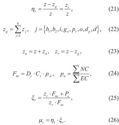
The goal of each business-manufacturing system is to have the optimum number of employees (zu) in both administration (za) and production (z). Investigations of the causes for losses in working hours and productive human resources utilization level ηr are of significance for workplaces and technological operations with prevailing manual work [19].

In order to identify and reveal regularities in causes for working hour losses, corresponding data were collected and analysed in human resources department in the year 2010. The human resources utilization level ηr, Eq. (21), and current losses (zj), per cause (j), were established based on handlers’ work records. The analysis indicated eight causes of working hour losses (j), Eq. (22): sick leave up to 30 days (b1), sick leave over 30 days (b2), unexcused absence from work and tickets out (i), holiday (go), downtime (e.g. lack of jobs, strikes, vis major) (pr),

paid and unpaid leave (o), national holidays (dp), and engagement in other jobs (d). The total number of employed workers (zu) is the sum of productive (z) and clerical (za) workers. The average number of productive workers present at work every day (zr) is the difference between the total number of productive workers and the average number of productive workers absent from work for all the abovementioned reasons (zg), Eq. (23). The scheduled norm hours (nh) load per worker (Fnc), coefficient of productive worker overtime engagement (ξr) and scheduled productive worker utilization level (μr) can be calculated by employing Eqs. (24) to (26).

η_r z zg r

z z

z

= − = , (21)

z_g z_j j b b i g p o d d

j o r p

= =

{

}

=

∑

1 8

1 2

, , , , , , , , , (22)

z_u = +z z_a, z_r = −z z_g, (23)

F D C p p NC

EC

nc = r⋅ s⋅ n, n=

∑

∑

ξ_r r nc e

r nc

z F P

z F

= ⋅ +

⋅ , (25)

µ_r =η ξ_r⋅ _r. (26)

The scheduled norm hours load per worker (Fnc) is obtained as the product of the total number of working days (Dr), effective working hours in a shift (Cs) and the average norm hour [nh] execution (pn) for the observed organizational unit and a corresponding time period. The average norm-hour is obtained when the executed norm-hours (NC) are divided by the engaged effective working hours (EC) of productive

Table 5. Productive human resources utilization level ηr, total zg and partial zj losses of working hours, and scheduled parameter values μr

z

[workers/year]

zj, j = {b1, b2, i, go, dp, pr, o, d} [%] zg

zr

[workers/year]

ηr

[%]

Pe

[nh/

year] Fnc ξr

zb₁ zb₂ zi z_go z_dp z_pr zo zd [%] [workers/_year]

1 2 3 4 5 6 7 8 9 10 11 12=1-11 13 14 15 16

800 6.15 1.8 1.35 11.4 2.85 1.8 1.35 0.3 27 216 584 73 163917 2217 1.13

F D C p

z F nc r s n

r r

= ⋅ ⋅ = ⋅ ⋅ =

= ⋅

257 7 5 1 15 2217. . [nh/worker annually],

ξ nnc e

r nc r r r

P z F

+

⋅ =

⋅ +

⋅ = = ⋅ = ⋅

584 2217 163917

workers per worksheet. The coefficient of overtime engagement depends on the specificity of workplaces and planned level of overtime hours (Pe).

Table 5 show parameters relevant to the utilization of productive human resources (PHR). Due to an adverse age structure, working hours losses are high on account of sick leave (b1, b2) and holiday (go). Of the total of 800 workers, 27% or 216 workers are, on average, absent from work. Productive human resource (PHR) utilization level amounts to 73%. Taking into account the coefficient of overtime engagement (ξr), the scheduled utilization level of PHR (μr) equals 82%.

3 MANUFACTURING CYCLES SCHEDULING

The optimization of manufacturing cycle times Tcp requires, first of all, investigations of losses causes, measurement of their values, minimization of their effects and scheduling of total losses Gcp to be lower than made Gcs, Fig. 5.

Fig. 5. Technological, scheduled and real manufacturing cycle time duration with corresponding losses

When scheduling the manufacturing cycles, the scheduled cycle duration Tcp should tend to the optimum, Fig. 5. In other words, the goal of scheduling as a cyclic process is to permanently tend to the minimization of total losses, which means that scheduled losses (Gcp) should always be less than generated (Gcs) in all optimization steps, Eq. (27).

T T G T T G T G

T T T G G

cp t cp cs t cs cp

t cp cs cp cs

= + = + = +

< < → <

, ,

. (27)

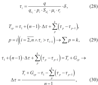
The scheduled manufacturing cycle duration

Tcp, Eq. (29), Figs. 6 and 7, aside from productive and non-productive cycle times, predicted by technological procedures, take into account scheduled manufacturing capacity utilization levels μi(μm, μr), Eqs. (20) and (26), real manufacturing conditions per operation, Eq. (28) and scheduled losses in a cycle (Gcp, ∆τ), Eq. (30).

τ

µ δ

i

s i d i i q

q p S_{i i} r

=

⋅ ⋅ ⋅ ⋅ ⋅ , (28)

T n

p i i n p k

cp p p

p k

i i

= +

(

)

(

)

=

(

)

−

−

∑

∑

τ τ τ τ

τ τ

1 1

1 1

2

∆ ,

, , (29)

τ τ τ τ

τ

τ τ τ

1 1

1 1

1

+

(

)

(

)

=

+ − −

(

)

−

−

∑

∑

n T G

T G

n p p p

k

t cp

t cp p p

p k

∆

∆

−−1 , (30)

where:

τi scheduled duration of technological operations, Δτ average partial loss between technological

operations,

p technological operation satisfying the condition from Eq. (29).

Fig. 6. Scheduled loss Δτi, τi > τi–1

Fig. 7. Scheduled loss Δτi, τi ≤ τi–1

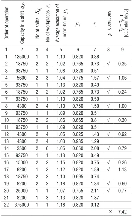
3.1 Algorithm for Cycle Scheduling

per technological operation (ri), the number of shifts per day (S_di), the average norm-hour execution (pi), manufacturing capacity utilization μi (μm, μr) and the norm-set capacity per shift (q_Si), Table 6. Inventories in unfinished production and losses due to quality inadequacy are included in calculations via the formulas for planning the quantity (q) of the product to be produced.

Table 6. Parameters for scheduling the manufacturing cycle

Order of operation

Capacity in a shif

t

qS i

No of shif

ts

Sd i

No of workplaces

ri

Average execution of nor

m-hours

pi

μi τi

p

operations _τ–p

τp–1

[calendar days]

1 2 3 4 5 6 7 8 9

1 125000 1 1 1.10 0.820 0.38

2 18750 2 2 1.02 0.765 0.73 √ 0.35 3 93750 1 1 1.08 0.820 0.51

4 5600 2 3 1.04 0.775 1.57 √ 1.06

5 93750 1 1 1.13 0.820 0.49

6 18750 2 2 1.02 0.765 0.73 √ 0.24 7 93750 1 1 1.10 0.820 0.50

8 4300 2 4 1.10 0.750 1.50 √ 1.00

9 93750 1 1 1.09 0.820 0.51

10 18750 2 2 1.06 0.665 0.81 √ 0.30 11 93750 1 1 1.09 0.820 0.51

12 4300 2 4 1.05 0.825 1.43 √ 0.92 13 4300 2 4 1.03 0.935 1.29

14 2500 2 6 1.05 0.650 2.08 √ 0.79 15 93750 1 1 1.13 0.820 0.49

16 15000 2 2 1.15 0.820 0.75 √ 0.26 17 8200 1 3 1.12 0.820 1.89 √ 1.13 18 18750 2 2 1.10 0.695 0.74

19 8200 2 2 1.18 0.820 1.34 √ 0.60 20 25000 1 1 1.07 0.755 2.11 √ 0.77 21 8200 1 3 1.13 0.820 1.87

22 375000 1 1 1.18 0.820 0.12

Σ 7.42

In the second step, it is necessary to adopt the total losses in the cycle Gcp, and, then using Eq. (30), to determine average partial losses between technological operations Δτ. Total scheduled losses in the cycle should be lower than those average (86.7 calendar days). They can be determined in a number of ways: by the help of Eq. (31) adopting the minimum value of losses in the cycle Gcs (Table 2, column 8).

G G G

G

cp cs cp

cs

≤ ≤

=

min , . ,

min min

39 4

41.4 102.4 132.4 ... 889.4

{

}

The scheduled value of total losses Gcp can be also found using Eq. (32).

G_{cp = −}T T_{c t}( )k_{. (32)}

The expected cycle time duration Tc will be calculated by applying Eqs. (6) or (7) if the values of the technological times per operation ti (Table 1, column 4) are corrected by the corresponding coefficients μi(Table 6, column 6). Data required for calculating the expected values of cycle duration Tc are given in Table 7.

According to the investigations [20], total losses in the cycle in the company follow the beta distribution, where the value Gc˝= Mo = 15.97 has the highest probability (modal value).

Based on the above analysis, total loss Gcp of 16 calendar days was adopted, and partial loss Δτ was calculated in calendar days, Eq. (33):

∆τ

τ τ τ

=

+ − −

(

)

− =

−

∑

T G

n

t cp p p

p k

1 1

1 2 2. . (33)

The third step implies calculating scheduled values for the cycle Tcp, in calendar days, using data from Table 6 and Eq. (29):

Tcp n p p

p k

= +τ1

(

)

∑

(

)

Correlation between real Tcs and scheduled Tcp manufacturing cycle time duration is determined by the flow coefficient Kp, Eq. (35).

K T

T p cs

cp

= . (35)

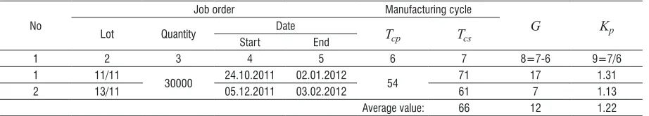
3.2 Production Launching According to the Scheduled Model and Analysis of Results

The scheduled mode of manufacturing (Tcp) was realized in two production lots (job order lot 11/11 and 13/11) in 2011 and 2012. In both job order lots, the quantity of 30,000 pieces each was launched. Prior to production initiation, in the ‘Term card’ document, the scheduled start and end dates for the manufacturing process per operation were recorded (with respect to the results obtained in Section 3.1).

on a current operation. Their value depends on the scheduled partial loss Δτ and organizational mode of production (Figs. 6 and 7). During production activities per technological operation, the start and end dates of production were added to the column denoting scheduled dates.

After production is finished according to the designed model, Table 8 shows realized manufacturing cycle time duration (Tcs), losses in the cycle (G) and values of the flow coefficient Kp, Relation (35).

Table 9 displays parameters (Tcs, G, Kp, Kt) for 15 job orders of the analysed part, whose production

was realized in the period from 2010 to 2012. In the first 13 job orders (Nos 1 to 13), the manufacturing cycle was not scheduled; therefore production process management was performed based on experience and priorities defined by operational managers.

The achieved values of the cycle Tcs (Table 9, column 5, Nos 14 and 15) are considerably lower than the analysed values of the cycles per job order (Table 9, column 5, Nos 1 to 13). The flow coefficient

Kp (1.13 to 1.31) takes considerably lower values than the coefficient Kt (2.02 to 5.18), which implies that Table 7. Parameters for calculating expected cycle time duration Tc

Order of operation

Machine code

Time per operation t_i [cmh/piece]

μi

Corrected time per operation [cmh/ piece]

Parameters for calculating technological cycle time

tk tj Fi (ti – ti–1)·Fi

1 2 3 4 5=3/4 6 7 8 9

1 - 6 0.820 7 - - 1 7

2 M1 40 0.765 52 52 - 1 45

3 - 8 0.820 10 - 10 0 0

4 M2 134 0.775 173 173 - 1 163

5 - 8 0.820 10 - 10 0 0

6 M1 40 0.765 52 52 - 1 42

7 - 8 0.820 10 - 10 0 0

8 M3 172 0.750 229 229 - 1 219

9 - 8 0.820 10 - 10 0 0

10 M4 40 0.665 60 60 - 1 50

11 - 8 0.820 10 - 10 0 0

12 M5 172 0.825 208 208 - 1 198

13 M6 172 0.935 184 - 184 0 0

14 M7 300 0.650 462 462 - 1 278

15 - 8 0.820 10 - 10 0 0

16 - 50 0.820 61 - - 1 51

17 - 92 0.820 112 112 - 1 51

18 M8 40 0.695 58 - 58 0 0

19 - 92 0.820 112 112 - 1 54

20 M9 30 0.755 40 - 40 0 0

21 - 92 0.820 112 112 - 1 72

22 - 2 0.820 2 - - 0 0

Σ 1522 - 1984 1572 342 - 1230

Eq. (6) →Tc = (1984 + 29999·(1572–342)) / 100000 / 6.866 = 53.74[calendar days/lot]

Eq. (32) →Gcp = 53.74 – 38.62 = 15.12 ≈16 [calendar days/lot]

Table 8. Parameters of the cycle established after production is finished according to the scheduled model

No

Job order Manufacturing cycle

G Kp

Lot Quantity Date T_cp T_cs

Start End

1 2 3 4 5 6 7 8=7-6 9=7/6

1 11/11

30000 24.10.2011 02.01.2012 54 71 17 1.31

2 13/11 05.12.2011 03.02.2012 61 7 1.13

the coefficient Kp is more suitable for measuring the production process efficiency than the coefficient Kt.

4 CONCLUSION AND FURTHER RESEARCH

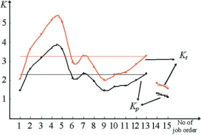
The goal of the original approach demonstrated in this work is to reduce manufacturing cycle time to the maximum, taking into account serial production characterized by discontinuity and the considerable amount of current assets needed for financing the production process. This methodology is based on designed models that, on one hand, respect current technical-technological and manufacturing documentation and, on the other, real production constraints. The parameters for reducing manufacturing cycle are flow coefficients Kp and Kt (Fig. 8).

When measured by flow coefficients Kp and

Kt, the average realized manufacturing cycle time duration, according to the designed model, is lower by 1.9 times (Table 9, columns 7 and 8), while the average losses in the cycle are smaller by 5.9 times (Table 9, column 6). Viewed from the angle of the manufacturing system, the flow coefficient Kp has a higher use value (Eq. (35)), because the accomplished values of the cycle are correlated with scheduled (planned) values. In this context, the model design becomes a cyclical process with the aim of minimizing total losses and reducing them to an optimal (i.e. acceptable) level. However, to compare the results with other business-manufacturing systems, from

the region and more distant areas, priority should be given to flow coefficient Kt, Eq. (16), because the values achieved for the cycle are compared to the technological (ideal) cycle, which is calculated for the case of serial production and combined workpiece move using Eqs. (6) or (7).

Fig. 8. Values of flow coefficients Kp and Kt per job order before and after scheduling

The results related to the identification of downtime causes and losses measurement are of importance not only for the cycle scheduling, but also for optimal production planning.

Further research should be directed to the analysis and scheduling of manufacturing cycle for complex products. It is necessary to define models for describing the structures of complex products Table 9. Values of the flow coefficients (Kp, Kt) before and after production launching according to the designed model

No Job order Manufacturing cycle and losses Kp Kt Production

Lot Quantity Tcp Tcs G

1 2 3 4 5 6= 5-4 7=5/4 8 9

1 04/10

30000 54

80 26 1.48 2.07

Experience-based production

2 05/10 141 87 2.61 3.65

3 06/10 171 117 3.17 4.43

4 07/10 200 146 3.70 5.18

5 08/10 195 141 3.61 5.05

6 09/10 114 60 2.11 2.95

7 10/10 127 73 2.35 3.29

8 01/11 104 50 1.93 2.69

9 03/11 78 24 1.44 2.02

10 04/11 89 35 1.65 2.30

11 05/11 93 39 1.72 2.41

12 06/11 109 55 2.02 2.82

13 07/11 128 74 2.37 3.31

Average value: 125.3 71.3 2.32 3.24

14 11/11

30000 54 71 17 1.31 1.84 Designed

model-based production

15 13/11 61 7 1.13 1.58

with respect to technological documentation and techniques that allow for the scheduling approach to realization of orders. The designed solutions, that are based on the principles of lean production, should make provisions for software application solutions from the domain of project management.

5 REFERENCES

[1] Slak, A., Tavcar, J., Duhovnik, J. (2011). Application of genetic algorithm into multicriteria batch manufacturing scheduling. Strojniški vestnik - Journal of Mechanical Engineering, vol. 57, no. 2, p. 110-124, DOI:10.5545/sv-jme.2010.122.

[2] Suzic, N., Stevanov, B., Cosic, I., Anisic, Z., Sremcev, N. (2012). Customizing products through application of group technology: A case study of furniture manufacturing. Strojniški vestnik - Journal of Mechanical Engineering, vol. 58, no. 12, p. 724-731. DOI:10.5545/sv-jme.2012.708.

[3] Eckert, C., Clarkson, P. (2010). Planning development

processes for complex products. Research in

Engineering Design, vol. 21, no. 3, p. 153-171, DOI:10.1007/s00163-009-0079-0.

[4] Alfieri, A., Tolio, T., Urgo, M. (2011). A project scheduling approach to production planning with feeding precedence relations. International Journal of Production Research, vol. 49, no. 4, p. 995-1020, DOI:10.1080/00207541003604844.

[5] Dossenbach, T. (2000). Manufacturing cycle time reduction - a must in capital project analysis. Wood & Wood Products, vol. 105, no. 11, p. 31-35.

[6] Johnson, J.D. (2003). A framework for reducing

manufacturing through put time. Journal of

Manufacturing Systems, vol. 22, no. 4, p. 283-298, DOI:10.1016/S0278-6125(03)80009-2.

[7] Lati, N., Gilad, I. (2010). Minimising idle times in cluster tools in the semiconductor industry. International Journal of Production Research, vol. 48, no. 21, p. 6443-6459, DOI:10.1080/00207540903280556. [8] Herrmann, J.W., Chincholkar, M.M. (2000). Design

for production: A tool for reducing manufacturing cycle time. Proceedings of the 2000 ASME Design Engineering Technical Conference, Baltimore, from: http://www.isr.umd.edu/Labs/CIM/projects/dfp/ dfm2000.pdf.

[9] Li, L., Chang, Q., Ni, J., Biller, S. (2009). Real time production improvement through bottleneck

control. International Journal of Production

Research, vol. 47, no. 21, p. 6145-6158, DOI:10.1080/00207540802244240.

[10] Patti, A.L., Watson, K.J. (2010). Downtime variability: the impact of duration-frequency on the performance of serial production systems. International Journal of Production Research, vol. 48, no. 19, p. 5831-5841, DOI:10.1080/00207540903280572.

[11] Schultz, C.R. (2004). Spare parts inventory and cycle time reduction. International Journal of Production Research, vol. 42, no. 4, p. 759-776, DOI:10.1080/0020 7540310001626210.

[12] Kusar, J., Berlec, T., Zefran, F., Starbek, M. (2010). Reduction of machine setup time. Strojniški vestnik - Journal of Mechanical Engineering, vol. 56, no. 12, p. 833-845.

[13] Berlec, T., Govekar, E., Grum, J., Potocnik, P., Starbek, M. (2008). Predicting order lead times. Strojniški vestnik - Journal of Mechanical Engineering, vol. 54, no. 5, p. 308-321.

[14] Ko, S.S., Serfozo, R., Sivakumar, A.I. (2004). Reducing cycle times in manufacturing and supply chains by input and service rate smoothing. IIE Transactions, vol. 36, no. 2, p. 145-153, DOI:10.1080/07408170490245441. [15] Puich, M. (2001). Are you up to the cycle-time

challenge?. IIE Solutions, vol. 33, no. 4, p. 24-28. [16] Hadas, L., Cyplik, P., Fertsch, M. (2009).

Method of buffering critical resources in make-to-order shop floor control in manufacturing

complex products. International Journal of

Production Research, vol. 47, no. 8, p. 2125-2139, DOI:10.1080/00207540802572582.

[17] Djukic, R., Jovanovic, R.J., Mutavdzic, M. (2009). Investigations of machine capacity utilization level, downtime causes and structure of losses. Proceedings of Jupiter Conference, Belgrade, p. 4.11-4.16. (in Serbian)

[18] Djukic, R., Milanovic, D., Jovanovic, R.J. (2010). Program for establishing machine capacity utilization level. Proceedings of Quality Conference, Kragujevac, from: http://www.cqm.rs/2010/pdf/37/37.pdf. (in Serbian)

[19] Djukic, R., Jovanovic, R.J. (2009). Effects of human resources on dynamic management of manufacturing systems. Proceedings of Jupiter Conference, Belgrade, p. 4.1-4.6. (in Serbian)