www.geosci-model-dev.net/10/1751/2017/ doi:10.5194/gmd-10-1751-2017
© Author(s) 2017. CC Attribution 3.0 License.
Accelerating volcanic ash data assimilation using a mask-state
algorithm based on an ensemble Kalman filter: a case study with the
LOTOS-EUROS model (version 1.10)
Guangliang Fu1, Hai Xiang Lin1, Arnold Heemink1, Sha Lu1, Arjo Segers2, Nils van Velzen1,3, Tongchao Lu4, and Shiming Xu5
1Delft University of Technology, Delft Institute of Applied Mathematics, Mekelweg 4, 2628 CD Delft, the Netherlands 2TNO, Department of Climate, Air and Sustainability, P.O. Box 80015, 3508 TA Utrecht, the Netherlands
3VORtech, P.O. Box 260, 2600 AG Delft, the Netherlands.
4School of Mathematics, Shandong University, Jinan, Shandong, China 5Department of Earth System Science, Tsinghua University, Beijing, China
Correspondence to:Guangliang Fu ([email protected])
Received: 1 August 2016 – Discussion started: 24 August 2016
Revised: 7 February 2017 – Accepted: 3 April 2017 – Published: 24 April 2017
Abstract. In this study, we investigate a strategy to accel-erate the data assimilation (DA) algorithm. Based on eval-uations of the computational time, the analysis step of the assimilation turns out to be the most expensive part. After a study of the characteristics of the ensemble ash state, we propose a mask-state algorithm which records the sparsity information of the full ensemble state matrix and transforms the full matrix into a relatively small one. This will reduce the computational cost in the analysis step. Experimental re-sults show the mask-state algorithm significantly speeds up the analysis step. Subsequently, the total amount of comput-ing time for volcanic ash DA is reduced to an acceptable level. The mask-state algorithm is generic and thus can be embedded in any ensemble-based DA framework. Moreover, ensemble-based DA with the mask-state algorithm is promis-ing and flexible, because it implements exactly the standard DA without any approximation and it realizes the satisfying performance without any change in the full model.
1 Introduction
Volcanic ash erupted into atmospheres can lead to severe in-fluences on aviation society (Gudmundsson et al., 2012). Tur-bine engines of airplanes are extremely threatened by ash in-gestion (Casadevall, 1994). Thus, accurate real-time aviation
advice is highly required during an explosive volcanic ash eruption (Eliasson et al., 2011). Using data assimilation (DA) to improve model forecast accuracy is a powerful approach (Lu et al., 2016a). Recently, ensemble-based DA (Evensen, 2003) has been evaluated as very useful for improving vol-canic ash forecasts and regional aviation advice (Fu et al., 2016). It corrects volcanic ash concentrations by continu-ously assimilating observations. In Fu et al. (2016), real air-craft in situ measurements were assimilated using the ensem-ble Kalman filter (EnKF), which is the best known and most popular ensemble-based DA method. Based on the validation with independent data, ensemble-based DA was concluded as being powerful for improving the forecast accuracy.
fore-casts has gained much attention, because it is needed to pro-vide timely and accurate aviation advice for frequently oper-ated commercial airplanes. It was shown that the accuracy of volcanic ash transport can be significantly improved by the DA system in Fu et al. (2016). Therefore, it is urgent to also consider the computational aspect, i.e., improving the com-putational speed of the volcanic ash DA system as quickly as possible. This is the main focus of this study.
Due to the computational complexity of ensemble-based algorithms and the large scale of dynamical applications, applying these methods usually introduces a large compu-tational cost. This has been reported from the literature on different applications. For example, for operational weather forecasting with ensemble-based DA, Houtekamer et al. (2014) reported computational challenges at the Canadian Meteorological Center with an operational EnKF featuring 192 ensemble members, using a large 600×300 global hor-izontal grid and 74 vertical levels. An initialization require-ment of over 7×10¹⁰values to specify each ensemble results in large computational efforts on the initialization and fore-cast steps in weather forefore-casting. For oil reservoir history-matching (Tavakoli et al., 2013), the reservoir simulation model usually has a large number of state variables; thus, the forecasts of an ensemble of simulation models are often time-consuming. Besides, when time-lapse seismic or dense reservoir data are available, the analysis step of assimilat-ing these large observations becomes very time-consumassimilat-ing (Khairullah et al., 2013). Large computational requirements of ensemble-based DA have also been reported in ocean cir-culation models (Keppenne, 2000; Keppenne and Rienecker, 2002), tropospheric chemistry assimilation (Miyazaki et al., 2015), and many other applications.
To accelerate an ensemble-based DA system, the ensem-ble forecast step can first be parallelized because the propa-gation of different ensemble members is independent. Thus if a computer with a sufficiently large number of parallel pro-cessors is available, all the ensemble members can be simul-taneously integrated. In the analysis stage, to calculate the Kalman gain and the ensemble error covariance matrix, all ensemble states must be combined together. In weather fore-casting and oceanography sciences, Keppenne (2000), Kep-penne and Rienecker (2002), and Houtekamer and Mitchell (2001) have reported using parallelization approaches to ac-celerate the expensive analysis stage. In reservoir history matching, a three-level parallelization has been proposed by Tavakoli et al. (2013); Khairullah et al. (2013) in recent years, to significantly reduce computational efforts of both fore-cast and analysis steps due to massive dense observations and large simulation models. The first parallelization level is to separately perform the ensemble simulations on different processors during the forecast step. This approach is usually quite efficient when a large ensemble size is used. However, the scale or model size of one reservoir simulation is con-strained by the memory of a single processor. Thus, the sec-ond parallelization level is to perform one ensemble member
simulation using a parallel reservoir model. These two lev-els do not deal with the analysis step, which collects all en-semble members to do computations usually on a single pro-cessor. Therefore, a third level of parallelization was imple-mented by Tavakoli et al. (2013) and Khairullah et al. (2013) by parallelizing matrix-vector multiplications in the analysis steps. Furthermore, some other approaches on accelerating ensemble-based DA systems have also been reported, such as GPU-based acceleration (Quinn and Abarbanel, 2011) in numerical weather prediction (NWP) and domain decompo-sition in atmospheric chemistry assimilation (Segers, 2002; Miyazaki et al., 2015). The observations used in an DA sys-tem can also be optimized with some preprocessing proce-dures, as reported by Houtekamer et al. (2014).
Although for other applications there were many efforts in dealing with large computational requirements in an ensemble-based DA system, most of them cannot be directly used to accelerate volcanic ash DA. This is because the accel-eration algorithms are strongly dependent on specific prlems, such as model complexity (high or low resolution), ob-servation type (dense or sparse), or primary requirement (ac-curacy or speed). These factors determine, for a specific ap-plication, which part is the most time-consuming, and which part is intrinsically sequential. Thus, no unified approach for efficient acceleration of all the applications can be found. Al-though the successful approaches in other applications can-not be directly employed in volcanic ash forecasts, their suc-cess does stress the importance of designing a proper ap-proach based on the computational analysis of a specific DA system. Therefore, the computational cost of our volcanic ash DA system will first be analyzed. Then, based on the compu-tational analysis, we will investigate a strategy to accelerate the ensemble-based DA system for volcanic ash forecasts.
This paper is organized as follows. Section 2 introduces the methodology of volcanic ash DA. Section 3 analyzes the computational cost of the conventional volcanic ash DA sys-tem. In Sect. 4, the mask-state algorithm (MS) is developed for acceleration. The comparison between MS and standard sparse matrix methods is presented in Sect. 5. The discus-sions on MS is in Sect. 6. Finally, the last section summarizes the concluding remarks of our research.
2 Methodology of the volcanic ash DA system
ac-curacy requirement of the volcanic ash forecasts to aviation advice as mentioned in Sect. 1.
To simulate a volcanic ash plume, an atmospheric trans-port model is needed. In this paper, the LOTOS-EUROS (abbreviation of LOng Term Ozone Simulation – EURo-pean Operational Smog) model is used (Schaap et al., 2008) with model version 1.10 (http://www.lotos-euros.nl/). The LOTOS-EUROS model (Schaap et al., 2008) is an opera-tional model focusing on nitrogen oxides, ozone, particu-late matter, and volcanic ash. The model configurations for volcanic ash were discussed in detail by Fu et al. (2016). For volcanic ash simulation, the model is configured with a state vector of size 180×200×18×6 (the dimensions cor-respond to longitude, latitude, vertical level, and ash species), and the size of the model state is thus calculated as∼106.
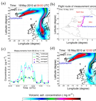
The experiment in this study starts at t0 (09:00 UTC, 18 May 2010 for this study) by considering an initial con-dition from a previous LOTOS-EUROS conventional model run (see Fig. 1a). In the second step (the forecast step) the model propagates the ensemble members from the timetk−1 totk(k >0, the time step is 10 min):
ξfj(k)=Mk−1(ξaj(k−1)). (1)
The operatorMk−1describes the time evolution of the state which contains the ash concentrations in all model grid boxes. The state at the time tk has a distribution with the
mean xf and the forecast error covariance matrix Pf given by
xf(k)= [
N
X
j=1
ξfj(k)]/N, (2)
Lf(k)= [ξf1(k)−xf(k),· · ·,ξfN(k)−xf(k)], (3) Pf(k)= [Lf(k)Lf(k)T]/(N−1), (4) whereLfrepresents the ensemble perturbation matrix. In this study, the forecast step is performed in parallel because of the natural/common parallelism of the independent ensem-ble propagation, which is a trivial approach when employing ensemble-based DA (Liang et al., 2009; Tavakoli et al., 2013; Khairullah et al., 2013).
When the model propagates to 09:40 UTC, 18 May 2010, the volcanic ash state gets sequentially analyzed by the DA process by combining real aircraft in situ measurements of PM10 and PM2.5concentrations until 11:10 UTC. The mea-surement route and values are demonstrated in Fig. 1b, c and the details are described in Weber et al. (2012) and Fu et al. (2016). The observational network at time tk is defined by
the operatorHk which maps the state vectorxto the
obser-vational vectoryby
y(k)=Hk(x(k))+v(k), (5)
whereycontains the aircraft measurements andvrepresents the observational error.Hk selects the grid cell inx(k)that
corresponds to the locations of the observation. When mea-surements are available, the ensemble members are updated in the analysis step using
K(k)=Pf(k)H(k)T[H(k)Pf(k)H(k)T+R]−1, (6) ξaj(k)=ξfj(k)+K(k)[y(k)−H(k)ξfj(k)+vj(k)], (7)
whereKrepresents the Kalman gain,His the observational matrix formed by the observational operator H, R repre-sents the measurement error covariance matrix, andvj
repre-sents the realization out of the observation error distribution v. After the continuous assimilation ending at 11:10 UTC, the forecast at 12:00 UTC is illustrated in Fig. 1d, for which the forecast accuracy has been carefully evaluated as signifi-cantly improved compared to the case without DA (Fu et al., 2016).
The EnKF with the above setups is abbreviated as “con-ventional EnKF” and used in this study for the computational evaluation. Note that in the study we do not use covariance localization as proposed by Hamill et al. (2001) for reducing spurious covariances. This is because although localization is possible, the ideal case is not to use it in order to have the correct covariances in a large (converged) ensemble. It is crucial for localization that when unphysical (spurious) co-variances are eliminated, physical (correct) coco-variances can be well maintained (Petrie and Dance, 2010). If the “filtering length scale” for localization is too long (i.e., all the dynam-ical covariances are allowed), many of the spurious covari-ances may not be eliminated. If the length is too short, im-portant physical dynamical covariances then may be lost to-gether with the spurious ones. Therefore, essentially deciding on an accurate localization is a challenging subject (Riisho-jgaard, 1998; Kalnay et al., 2012), especially for accuracy-demanding applications. Therefore, in this study we choose the ensemble size of 100 to guarantee the accuracy and avoid large spurious covariances.
3 Computational analysis for volcanic ash DA 3.1 Computational analysis of the total runtime Ensemble-based DA is a useful approach to improve the fore-cast accuracy of volcanic ash transport. However, if it is time-consuming, it cannot be taken as efficient due to the high re-quirement on speed for volcanic ash DA (see Sect. 1). Based on this consideration, we need to analyze the computational cost of a conventional volcanic ash DA system.
fore-Figure 1.Methodology of ensemble-based DA.(a)The initial volcanic ash state at 09:00 UTC.(b)Flight route of measurement aircraft. (c) Aircraft in situ measurements of PM10 and PM2.5from 09:30 to 11:10 UTC, 18 May 2010. (d)Volcanic ash assimilation result at 12:00 UTC.
cast time is obtained from Eq. (1), while the analysis time corresponds to the computational sum from Eqs. (2) to (7). The other computational time includes script compiling, set-ting environment variables, and starset-ting and finalizing DA algorithms.
The evaluation result of the conventional EnKF is shown in Table 1 (the middle column). It can be seen that the total computational time (4.36 h) is relatively large compared to the simulation window (3.0 h, i.e., from 09:00 to 12:00 UTC, 18 May 2010), which is too much in an operational sense. Therefore, in this study, we aim to accelerate the computation to within an acceptable runtime (i.e., requiring less runtime than the time period of the DA application).
It can also be observed from Table 1 that the main contri-bution to the total execution time is the analysis step. Com-pared to the initialization and forecast time, the analysis stage takes 72 % of the total runtime. Due to the expensive analy-sis step, although some approaches (such as MPI-parallel I/O Filgueira et al., 2014, domain decomposition Segers, 2002) can potentially accelerate the initialization and forecast step,
the effect on the final acceleration of the total computational cost is little. Therefore, to get an acceptable computational time, the cost reduction in the analysis step is the target. One may wonder that since the number of observations is small, why does analysis take so much time? The large state vec-tor seems to be left responsible for the problem. To know the exact reason, the detailed computational cost of the analysis step must be evaluated.
3.2 Cost estimation of all analysis procedures
We start with the formulations of the analysis step. The anal-ysis step is represented by Eq. (7), which can be written in a full matrix format with Eq. (8),
Aan×N=Afn×N+Kn×m(Ym×N−Hm×nAfn×N), (8)
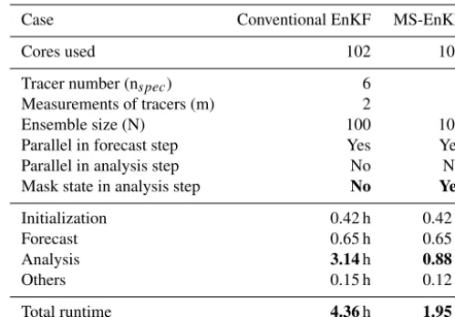
Table 1.Comparison of the computational cost of conventional EnKF and MS-EnKF. (The results are obtained from the bullx B720 thin nodes of the Cartesius cluster, which is a computing facility of SURFsara, the Netherlands Supercomputing Centre. Each node is configured with 2×12-core 2.6 GHz Intel Xeon E5-2690 v3 (Haswell) CPUs and with memory 64 GB.)
Case Conventional EnKF MS-EnKF
Cores used 102 102
Tracer number (nspec) 6 6
Measurements of tracers (m) 2 2
Ensemble size (N) 100 100
Parallel in forecast step Yes Yes
Parallel in analysis step No No
Mask state in analysis step No Yes
Initialization 0.42 h 0.42 h
Forecast 0.65 h 0.65 h
Analysis 3.14h 0.88h
Others 0.15 h 0.12 h
Total runtime 4.36h 1.95h
h: hour; simulation window =3.0h; the time is wall clock time.
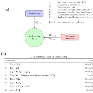
by an ensemble ofy+v(see Eq. 7).His the observational matrix, which is used to select state variables (at measure-ment locations) in the full ensemble state matrix correspond-ing to the measurement ensemble matrixY.nis the number of model state variables in a three-dimensional (3-D) domain, i.e.,∼106in this study (see Sect. 2).mis the number of mea-surements at one assimilation time, which depends on the measurement type. For aircraft in situ measurements used in this study (see Fig. 1c), two measurements are made at each time by one research flight, so thatmis 2 here.N is the en-semble size and is taken as 100 in this study. As described in Eq. (3), the ensemble perturbation matrixLfin EnKF can be re-written as
Lfn×N=Afn×N− ¯Anf×N=Afn×N(IN×N−
1
N1N×N)
=Afn×NBN×N, (9)
whereI is anN ×N unit matrix and1 is anN ×N ma-trix with all elements equal to 1. Thus, Lf=AfB where BN×Nis introduced to represent(IN×N−N11N×N), so that
HLf=OfB, whereOf
m×Nis used to represent (HA
f). Here we explicitly expressLfandHLfin the form ofAfandOf, respectively. This is because in our volcanic ash DA system, AfandOfare two of the three inputs (another one is the mea-surement ensemble matrixYfor the analysis step). These are the three inputs used for actual computations in the analysis step. As shown in Fig. 2a,Afis obtained from the forecast step, andOfandYare acquired from our stochastic observer module (see Fig. 2a) which is used for a volcanic ash trans-port model to integrate geophysical measurements. With the inputY, the measurement error covarianceR, as introduced
in Eq. (6), can then be computed with
Rm×m=
1
N−1(Ym×N− ¯Ym×N)(Ym×N− ¯Ym×N)
0
= 1
N−1(YB)(YB)
0
. (10)
Based on previous definitions and Eqs. (2) to (7), the anal-ysis step can be reformulated as follows:
Aan×N=Af+K(Y−HAf)
=Af+PfH0(HPfH0+R)−1(Y−HAf)
=Af+ 1
N−1L
f(HLf)0[ 1
N−1(HL f)(HLf)0
+ 1
N−1(YB)(YB)
0]−1(Y−HAf) (11)
=Af+AfB(OfB)0[(OfB)(OfB)0
+(YB)(YB)0]−1(Y−Of)
=Af{I+B(OfB)0[(OfB)(OfB)0
+(YB)(YB)0]−1(Y−Of)} =Afn×NXN×N,
where
XN×N= {I+B(OfB)0[(OfB)(OfB)0
Figure 2.Computational evaluation of the analysis step.(a)Illustration of the analysis step.(b)Computational cost of all sub-parts of the analysis step.
each procedure in the analysis step. Considering that the state numbern (∼106) is significantly larger than the measure-ment numberm(m=2 here) and the ensemble sizeN(N=
100), the most time-consuming procedure in the analysis step is thus the last one, that isAa=AfXwith a computational cost of O(n N2). Therefore, in our volcanic ash DA system, this part is the most time-consuming part in the analysis step. Note that the procedure [(OfB)(OfB)0+(YB)(YB)0]−1for singular value decomposition (SVD) in our study is not time-consuming, which is different from applications of reservoir history matching (Tavakoli et al., 2013; Khairullah et al., 2013). This is because of the SVD procedure costs O(m3), and due to the measurement size on the order of the size of the state in those cases, the SVD procedure thus requires a huge computational cost for reservoir DA.
4 The mask-state algorithm (MS) for acceleration of the analysis step
4.1 Characteristic of ensemble state matrix Af
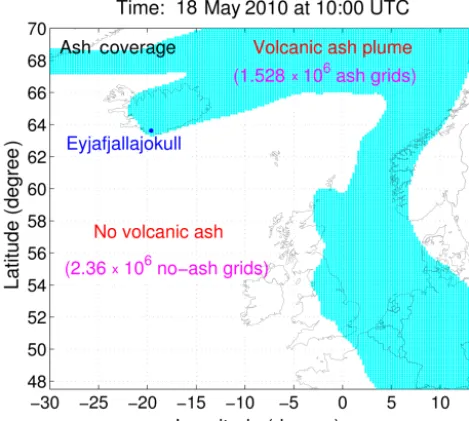
Figure 3.Characteristics of a volcanic ash state.
in contrast to other atmospheric-related applications such as ozone (Curier et al., 2012), SO2(Barbu et al., 2009), and CO2 (Chatterjee et al., 2012). For those applications, the concen-trations are everywhere in the domain, the emission sources are also everywhere, and observations are available through-out the domain too (especially for satellite data), whereas for application of volcanic ash transport, the source emission is only at the volcano; thus, usually only a limited domain is polluted by ash. As shown in Fig. 3, in the 3-D domain with a grid size of 3.888×10⁶, the number of grids in the area with volcanic ash is counted as 1.528×10⁶, whereas the number of no-ash grids is 2.36×10⁶. Note that shown in the figure are accumulated ash coverages of all ensemble states; thus, in the no-ash grids, there is no ash for any of the ensemble states. Thus a very large number of rows inAfare zero corre-sponding to the no-ash grids. These zero rows inAfhave no contributions toAa=AfX, because a zero row inAfalways results in a zero row inAa. Therefore, for the case of Fig. 3, 2/3 of the computations are redundant and can be avoided. To realize this, one may think to limit the domain for the en-tire assimilation step; then, the number of zero rows certainly would be largely reduced. This is actually incorrect, because these zero rows are changing along with the transport of ash clouds, and are not constant at each analysis step. So the full domain must be considered and it should be adaptive (choose different zero rows according to differentAfat different anal-ysis times).
4.2 Derivation of the mask-state algorithm (MS) Here we introduce item nnoash to represent the number of zero rows in the ensemble state matrix Af, and usenash to represent the number of other rows (also, nash represents
Figure 4.Algorithms for CSR-based SDMM to compute the mul-tiplication of sparse matrixAfand dense matrixX.(a) Multiplica-tion ofAfby a column vectorv(inX) by CSR-based sparse matrix vector multiplication (SpMV).val,col_idx, androw_ptrare the three arrays to representAfin CSR format.(b)Looping SpMV N times (each with one column ofX) to obtainAa=AaX.
the grid size of ash plume). When computingAa=AfX, to avoid all the computations related tonnoash rows with zero elements, the index of othernashrows must first be decided. This index is meant to reduce the dimensions ofAf. After getting aAawith a dimension ofnash×N, the index will be used again to reconstruct the full matrixAawith the dimen-sion ofn×N. Based on this idea, we propose a mask-state algorithm (MS) which deals with the time-consuming analy-sis update. MS includes five steps.
i. Compute ensemble mean state A¯f. The mean state
¯
Afn×1 can be easily computed by averaging Afn×N alongN columns. Due to all elements inAfn×N corre-sponding to ash concentrations, all elements inAfn×N are larger than or equal to zero. The index of non-zero rows inA¯fn×1is thus equivalent to that inAfn×N. The computational cost for this step is O(n N).
ii. Construct mask arrayz. Based on previously obtained
¯
iii. Construct masked ensemble state matrixeAf. Using the mask arrayznash×1obtained from step (ii),eA
f
nash×Ncan be constructed column by column according to Eq. (13), and the computational cost (overhead) for this step is O(nashN).
e
Af(1:nash,1:N )=Af(z(1:nash),1:N ) (13) iv. ComputeeAa by multiplyingeAfandX. Perform matrix
computation eAan
ash×N=eA f
nash×NXN×N. This step is similar toAa=AfX, as described in Sect. 3.2, but the computational cost now becomes O(nashN2) instead of O(n N2).
v. Construct analyzed ensemble state matrixAa. With the computedeAa from step (iv) and the mask arrayzfrom step (ii), the final analyzed ensemble state matrixAan×N can be constructed based on Eq. (14). The computa-tional cost (overhead) for this step is O(n N).
Aa(z(1:nash),1:N )=Aea(1:nash,1:N ) (14) According to the derivations of MS, the computational costs related to zero rows are avoided. Here the “zero rows” do not equal “zero elements”. The former corresponds to the regions where there is no ash for all the ensemble members, while the latter also counts the no-ash regions specifically for some ensembles. Certainly the consideration of all “zero ele-ments” can include all the sparsity information of the ensem-ble state matrix, but extra computations and memories must be spent on searching the full matrixAf
n×Nwith a
computa-tional cost of O(nN) and storing a mask-state matrix with di-mensions ofn×N. This is expensive compared to construct-ing the mask array in procedure (ii). Actually, after a careful check of the volcanic ash ensemble plumes, there is no “bad” ensemble which is really different from others. Although the concentration levels in ensemble members are distinct, the main direction and the occurrence to the grid cells are more or less the same. This means that the “zero rows” actually more or less equal “zero elements” but are much faster than the way with “zero elements”, which confirms the suitabil-ity and advantage of procedure (ii). Probably when there are big meteorological uncertainties, the “zero elements” will be much larger than “zero rows”. In this case, how to make use of the sparsity information in the ensemble state matrix will be considered in future.
Based on procedures of MS, the computational cost of Aa=AfXcan be reduced. However, without a careful eval-uation, we cannot conclude MS is fast, because the algo-rithm also employs other procedures. If these procedures (i), (ii), (iii), and (v) are much cheaper than the main procedure (iv), MS can definitely speed up the analysis step, and vice versa. Now we analyze MS’s computational cost, which can be summed as O(n N) + O(n) + O(nashN) + O(nashN2) + O(n N), i.e., O(n N+nashN2). Thus, the computational over-head involved in transforming the full matrix to a small one
(i.e., O(nashN) for procedure (iii)) has little effect on the to-tal computation cost of MS (i.e., O(n N+nashN2)). However, the computational overhead of transforming the small matrix to the full one (i.e., O(n N) for procedure (v)) does contribute a part, which cannot be ignored, to the total MS’s computa-tional cost. The computacomputa-tional cost without MS is O(n N2).
The comparison between both costs (with and without MS, i.e., O(n N+nashN2) and O(n N)) indicates when the number of non-zero rows (nash, i.e., the number of grids with ash) of the forecasted ensemble state matrix satisfies nash < NN−1n; then, MS can accelerate Aa=AfX. Here, O(n N+nashN2) and O(n N) are on the same order when nash < NN−1n. The larger the difference betweennash and
N−1
N n, the better the speedup can be achieved. According
to this analysis, and the characteristic (e.g., nash
n
approxi-mately equals13in this case) of volcanic ash transport as de-scribed in Sect. 4.1, the relation is certainly satisfied and is actuallynash NN−1n(significantly smaller) for our study. Therefore, for our volcanic ash DA system, with MS, the computational cost for the time-consuming partAa=AfX is O(nashN2), which is much reduced compared to O(n N2) with conventional computations.
The relation nash < NN−1n indicates whether we would have speedup by the MS method; actually, it can be extended to Eq. (15),
Sms= O(n N
2) O(n N+nashN2)
=O
n nash
, (15)
which explicitly specifies the expected amount of speedup (Sms) ofAa=AfXby the MS algorithm. In this case study, Nis taken at 100 andnash
n ≈
1
3, soSmsis approximately 3.0. According to Amdahl’s law (Amdahl, 1967), the total computational speedup (Stotal) by MS can be predicted by Eq. (16),
Stotal=
1 (1−pms)+pSmsms
, (16)
where pms is the proportion of the computational cost of Aa=AfXin the overall DA computations. It has been evalu-ated that the computational cost ofAa=AfXdominates the analysis step (see Fig. 2b); thus, the proportion of the compu-tational cost ofAa=AfXapproximates the proportion of the analysis step in the total DA computations (i.e.,pms ≈72 % in this case, as described in Sect. 3.1). Therefore, based on Eq. (16), the maximum (“ideal”) computational speedup can be predicted to be 1−1p
ms (i.e., ≈3.57 for this case study) whenSmsapproximates infinity. However, this is not the ac-tual speedup becauseSms is in fact specified by Eq. (15). Based on the discussions above,Stotal can therefore be es-timated by Eq. (15) at≈2.0 in this case.
4.3 Experimental results
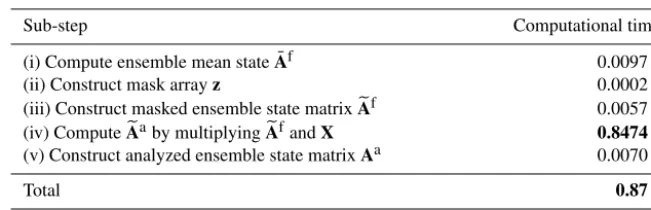
Table 2.Computational evaluation of all the steps of the mask-state algorithm (MS) forAa=AfX. (See the details of each step of MS in Sect. 4.2.)
Sub-step Computational time
(i) Compute ensemble mean stateA¯f 0.0097 h
(ii) Construct mask arrayz 0.0002 h
(iii) Construct masked ensemble state matrixeAf 0.0057 h
(iv) ComputeeAaby multiplyingeAfandX 0.8474h
(v) Construct analyzed ensemble state matrixAa 0.0070 h
Total 0.87h
h: hour; the time is wall clock time.
the time-consumingAa=AfX. Now MS will be applied in the real volcanic ash DA system, to investigate whether in practice it can speed up the analysis step well. We perform MS in the conventional EnKF, which means initialization and forecast steps are all computed as the conventional EnKF. The only difference between MS-EnKF and conventional EnKF is that in the former MS is employed for the analy-sis step, and in the latter is the standard analyanaly-sis step. The result and related specifications are shown in Table 1. As in-troduced in Sect. 2, the forecast step has been configured with the conventional parallelization; thus,N+2 (102 here) cores are actually used (one core for the DA algorithm, the other N+1 cores for the parallel forecast ofN ensemble members and one ensemble mean). It can be seen from Table 1 that MS indeed largely accelerates the analysis step (as expected, by a factor of about 3.0 for this study), which confirms the the-oretical cost evaluation. The detailed experimental time for each step of MS is shown in Table 2. As expected, the dense– dense matrix multiplication in step (iv) takes the largest part (i.e., 0.8474 h for this case study) of the total computational time (0.87 h) of MS. However, step (iv) has been a big im-provement compared to the case without MS (3.14 h; see Table 1), which is because the computational time for the other steps (e.g., steps (i–iii) cost only 0.0156 h to reduce the size of the ensemble state matrix) is little and ignorable. Note that the total computational time ofAa=AfXwith MS (i.e., 0.87 h in Table 2) is not exactly equal to the computa-tional time of the MS-EnKF analysis procedures (i.e., 0.88 h in Table 1). The subtraction (i.e., 0.01 h) corresponds to the summed computational time of all the other analysis proce-dures (i.e., proceproce-dures 1–8) except forAa=AfX(see Fig. 2b and Table 3).
MS is now experimentally proven as efficient to signifi-cantly reduce the computational time for the analysis step during volcanic ash DA. Note that it can also be observed that the computational time for the “other” parts in Table 1 (such as operations for setting environmental variables, start-ing and finalizstart-ing DA algorithms, as mentioned in Sect. 3.1) is slightly reduced by the MS method (i.e., 0.03 h in this case). This is because in the conventional EnKF, the
ensem-ble mean stateA¯fis calculated in the “other” parts as an out-put to finalize the DA algorithms, while in MS-EnKF, the calculations ofA¯f are needed and directly involved in the “Analysis” part.
The result shows that, benefitting from the success of a reduced analysis step, the overall computational cost indeed gets significantly reduced. The total execution time is 1.95 h, which is less than the simulation window of 3 h (09:00– 12:00 UTC, 18 May 2010). This result satisfies our goal to accelerate the computation to an acceptable runtime (i.e., re-quires less runtime than the time period of the DA applica-tion). Therefore, aviation advice based on the MS-EnKF can be provided as not only accurate, but also sufficiently fast. Note that the result (1.95 h) is obtained after the volcanic ash is transported to continental Europe. If the assimilation is performed in the starting phase of volcanic ash eruption (when aircraft measurements are available), a more signifi-cant acceleration would be obtained. This is because in this case the volcanic ash is only transported in an area near to the volcano; thus, the number of no-ash grid cells will take a large proportion (much higher than 2/3 for this case study) of the full domain.
There is another interesting point. According to Fig. 3, the ash grids comprise 39.3 % of the total grids. Thus, the min-imum computing time by using MS to utilize this model’s characteristic should be ≈1.234 h (i.e., 0.393×3.14 h). However, the experimental result shows that the computa-tional time goes down to 0.88 h (see Table 1). One reason for this time decrease is that when the size of the matrix is re-duced, the memory access cost also goes down (e.g., through better cache usages). Another possible reason is that the ash grid number actually decreases with time (not always taking 39.3 % of the total grid number), due to ash sedimentation and deposition processes (Fu et al., 2015).
Table 3.Computational time for the analysis step of conventional EnKF, MS-EnKF, and CSR-based-SDMM-EnKF.
Analysis procedures (see Fig. 2b) Conventional EnKF MS-EnKF CSR-based-SDMM-EnKF
procedures 1–8 0.01 h 0.01 h 0.01 h
procedure 9 (Aa=AfX) 3.13h 0.87h 1.21h
Total 3.14h 0.88h 1.22h
h: hour; the time is wall clock time.
the important aggregation process (Folch et al., 2010), there are big dependencies between different ash components and thus it does not make much sense to parallelize them. As for domain-decomposed parallelization (Segers, 2002), it is not efficient for our application. This is because volcanic ash is special in the sense that the model is only doing computa-tions in a small part of the domain (i.e., there are no data in a rather large part of domain), and this active part is con-tinuously changing. Thus, a fixed domain decomposition is not very useful here because of the changing plume posi-tion. In this sense, some advanced approach such as adaptive domain-decomposed parallelization (Lin et al., 1998) should be adopted to achieve additional acceleration to the volcanic ash forecast stage. This is an interesting subject for future ap-plication, when a more complicated model is employed, only ensemble parallelization may be not enough for the forecast stage.
5 Comparison between MS and standard sparse matrix methods
5.1 Issues related to the generation of CSR-based arrays
According to Sect. 4, MS has proven to be capable of solv-ing the computational issue ofAa=AfX. Motivated by the model’s characteristics, MS was proposed from an applica-tion’s perspective and achieved a good result by managing the irregular sparsity in our complicated volcanic ash DA system. The main reason why MS is efficient is that the sparsity of Af can be well utilized by MS. In Sect. 4, we only performed the comparison between MS and the case of full storage dense matrices. However, the problem abstracted here (AfX) is actually a sparse–dense matrix multiplication (SDMM) problem, since Af is sparse and Xis dense (see Eq. 12 forX). Thus, one may wonder what the result would be if the comparison of MS is made to more standard sparse matrix methods, such as compressed sparse row (CSR)-based methods (Saad, 2003; Bank and Douglas, 1993), which are commonly used for sparse matrix vector/matrix multiplica-tion.
Before we make the comparison, we need to first address the intrinsic problem when considering standard sparse ma-trix methods in EnKF for Aa=AfX. The issue is that it is
not possible to directly generate a sparse storage format (e.g., CSR) ofAfwithout first generating the full matrixAf. This is mainly becauseAfcomes from the model-driven ensem-ble forecast step, where eachAfcolumn corresponds to one member of the ensemble. During model forecast, we know there are indeed no-ash grids. However, it is not certain where the plume is exactly after one forecasting time step. This is highly dependent on the weather conditions and the model processes (e.g., advection and diffusion for horizontal grids, sedimentation and deposition for vertical grids). Thus, a fixed and wide domain is usually needed by the model to avoid complications, resulting in the generation of the full storage of Af (to be used inAa=AfX). Therefore, if we want to implement a CSR storage format for the sparse matrixAf, we must first generate the full storageAf from the ensem-ble forecast step, and then we generate the three CSR arrays based onAf.
Generating CSR arrays is usually much more expensive (computationally) than a single sparse matrix-vector multi-plication (SpMV). Thus, if we generate CSR arrays for only performing one-time SpMV, it would be meaningless from HPC’s point of view. Fortunately, this is not the case for Aa=AfX(i.e., SDMM), which can actually be considered as N-times SpMV. (Here,Xhas N columns, and one SpMV means the multiplication ofAfby one column ofX.) Thus, CSR-based SDMM might also be a candidate in reducing the computation time ofAa=AfX. It remains interesting to compare the performance of CSR-based SDMM and MS in dealing withAa=AfXfor our study case.
5.2 Result of CSR-based SDMM
To implement CSR-based SDMM forAa=AfX, the three CSR arrays forAf(denotedval,col_idx, androw_ptr in this study) need first to be generated. The arrayval of size nval stores non-zero values ofAf, wherenval ≈nashN. (In this study case, n= 3.888×10⁶,nash ≈ 1
3n, and N= 100.) The arraycol_idx of the same sizenval stores the column index of the non-zeros. The arrayrow_ptr saves the start and end pointers of the non-zeros of the rows inAf. The size ofrow_ptrisn+ 1.
Algo-rithm 1 forN times to obtainAa=AfX. The experimental result of CSR-based SDMM is shown in Table 4, where all the environmental conditions (such as the DA system, the programming environment) are the same as the case of MS. This gives a fair comparison between CSR-based SDMM and MS. In addition, for a pure algorithmic comparison with the serial MS, here the CSR-based SDMM is also performed in a serial case.
From Table 4, we can first confirm that the computational time (i.e., 0.0407 h) for the generation of the three CSR-based arrays (val,col_idx, androw_ptr to represent the sparse matrixAf) indeed takes more time than the computa-tional time of one CSR-based SpMV (i.e., 0.0117 h). Thus, there is little value in performing sub-step (i) (see Table 4) if only one SpMV (i.e., sub-step (ii)) is needed. However, to get allN (i.e., 100) columns ofAa, the sub-step (ii) is looped forN times, resulting in an ignorable impact of sub-step (i) on the total computational time (i.e., 1.21 h) of CSR-based SDMM.
The result of CSR-based SDMM also shows that the stan-dard sparse matrix methods can reduce the computational time ofAa=AfX, by comparing with the conventional way in Table 3. However, it can also be observed that the compu-tational time of CSR-based SDMM is larger than MS (i.e., 1.21 h versus 0.87 h in Table 3). Thus, although application of sparse matrix multiplication methods is positive, it is still slower than MS on our problem.
5.3 Comparison between CSR-based SDMM and MS In the CSR-based SDMM, only non-zero elements inAf par-ticipate in the multiplication betweenAfandX; thus, redun-dant computation (related to zero elements inAf) is avoided. So the computation time ofAfXis reduced with CSR-based SDMM. In the following, we analyze the performance differ-ence between CSR-based SDMM and MS.
Firstly, from the programming’s perspective, in CSR-based SDMM, the loop number for the rows ofAf is from 1 ton (see Fig. 4a), while the corresponding loop number in MS is from 1 to nash (see step (iv) of MS in Sect. 4.2, nash ≈(1/3)n). Although only non-zero elements are used in the multiplication in CSR-based SDMM, the length of the outer loop is still n (much larger than nash), which is the essential reason that MS is faster than CSR-based SDMM. Note that as discussed in Sect. 4.1, there are many zero rows inAf; thus, CSR-based SDMM actually does nothing when it comes to a zero row, but still needs to execute the loop. Within each loop number, it has to check the information fromrow_ptr (sizen+1), where the value corresponding to a zero row is usually set to be the value inrow_ptr cor-responding to the first subsequent non-zero row.
Secondly, with respect to the algorithm, CSR-based SDMM utilizes the sparsity ofAfby its generation of three CSR arrays, while MS not only utilizes the sparsity informa-tion of the sparse matrixAf, but also utilizes the consistency
of ensemble forecasts; that is, ensemble forecasted states are not consistent in values but usually consistent in non-zero locations. This is a typical property in ensemble-based DA, resulting inN ensemble plumes being different in concen-tration values but having similar transport directions/shapes (see Sect. 4.2). Thus, most of the zero elements in Af are actually in zero rows ofAf for an EnKF application, which leads to a small number of non-zero rows (nash) compared to the full number of rows (n) ofAf. Therefore, only con-sideringnashrows ineAfn
ash×NXN×N(see step (iv) of MS in Sect. 4.2) is more advantageous for an EnKF application than considering allnrows in CSR-based SDMM. Based on the above analysis, MS can be considered a specific sparse ma-trix method, which typically works for ensemble-based DA applications.
It is useful to apply standard sparse matrix methods (e.g., CSR-based SDMM) for our assimilation application. The ac-celerated analysis step by CSR-based SDMM (1.22 h; see Ta-ble 3) also reduces the total computational time (i.e., 2.29 h; see Table 1 for the computational time of initialization, fore-cast, and others) to an acceptable level (i.e., less than 3 h for our case study). In practice, due to the better performance of MS than CSR-based SDMM, we will use MS as a better choice for assimilation applications. In addition, we do not only intend to present MS, but also intend to reveal which part is the most time-consuming part for plume-type assimi-lation of in situ observations.
6 Discussions on MS 6.1 Applicability
Table 4.Computational evaluation of the sub-steps of the sparse–dense matrix multiplication with compressed sparse row storage (CSR-based SDMM) forAa=AfX.
Sub-step Computational time
(i) Compute three arrays (in CSR format) ofAf 0.0407 h (ii) Compute CSR-based SpMV for the first column ofAa 0.0117 h (iii) Loop (ii) for N-1 times for other N-1 columns ofAa 1.1576h
Total 1.21h
CSR-based SDMM is formed by (ii) and (iii). h: hour; the time is wall clock time.
many very low concentrations can be explicitly truncated to be zeros.
It has been analyzed that when the number of non-zero rows (nash, i.e., the number of ash grids in a 3-D domain) of Afsatisfies nash < n, MS can work faster than standard EnKF. For volcanic ash application, because nash is much less thann, the acceleration is quite large. Hence, in this case, we propose to embed MS in all ensemble-based DA methods because it is fast and the implementation using MS is exact to the standard ensemble-based methods; i.e., it does not intro-duce any approximation in view of MS procedures. Actually this proposal can be extended to all real applications, even if the condition is not satisfied. This is because in this case the computational cost of MS forAa=AfXbecomes O(n N2), which is the same as that of using the standard assimilation (shown in Fig. 2b). Therefore, if the state numbers are equal to or close to the total number of grid points in the domain, the added computational cost of using MS is very small (neg-ligible), so that the computational time with MS is almost the same as the time of using the standard approach, whereas when the conditionnash < nis satisfied, MS will accelerate the analysis step. Thus MS is generic and can be directly used in any ensemble-based DA, and this acceleration can be au-tomatically realized for some potential applications, without spending time investigating whether the condition is satis-fied. In a real (or operational) 3-D DA system, MS can be easily included; i.e., we only need to invoke the MS module when computingAa=AfX, without any other change to the current framework. Note that MS is applicable in ensemble-based DA but not in variational-ensemble-based DA. This is because in a variational-based DA system, the minimization of a cost function is mostly operated within several/many continuous time steps (Lu et al., 2016b, 2017); thus, it is convenient to always use the full (i.e., non-masked) domain to represent different state matrices (corresponding to different time steps in variational-based DA).
As stated in Eq. (15), the speedup of the MS method is ap-proximately the inverse of nash
n . So far there are no statistical
data on the value ofnash
n . Considering the problem of volcanic
ash transport, there is one emission point (at the volcano); all the ashes in atmospheres are transported by the directional wind drive from the same source point. Thus volcanic ash cloud is actually transported in a shape of a plume, which in
general does not cover the full but only a small part of the 3-D domain. At the start phase of a volcanic ash eruption,nash
n
is much smaller than 1.0 (started from 0). During transport over a long time (1.5 months for this case study), nash
n
in-creases to approximately 1/3. Therefore, the speedup of MS in ensemble-based volcanic ash DA will be significant.
6.2 MS and localization
Based on the formulation of MS, one may think it can be taken as a localization approach (Hamill et al., 2001). There is indeed a similarity between MS and the localization ap-proach, in a sense that when computingAa=AfX, both get rid of a large number of cells and only do computations re-lated to the selected grids. These two algorithms are however functionally different. This is because the localization ap-proach is meant for reducing spurious covariances outside a local region which is built up around the measurement; thus, the results with and without localization approaches are dif-ferent, while MS is developed for the acceleration purpose. The masked region is discontinuous and independent of loca-tions of measurement, but dependent on the model domain. Thus, there is no difference in the assimilation results be-tween using MS and without using it. Therefore, based on the functional difference, MS cannot be taken as a localiza-tion approach.
In this study, we do not employ the localization strategy in the analysis step, because we use a rather large ensemble size of 100 to guarantee the accuracy, as introduced in Sect. 2. But for some applications (e.g., ozone, CO2, sulfur dioxide), especially when assimilating satellite data, localization is a necessary approach and has been widely used in reducing spurious covariances (Barbu et al., 2009; Chatterjee et al., 2012; Curier et al., 2012). In these cases, because the local-ization approach forces the analysis only to update the state within a localization region, one may think that localization could replace MS and that there would be no significance in employing MS. Actually this is not correct. We explain the reason as follows.
1998, 2001) given by
K(k)=(f◦Pf(k))H(k)T[H(k)(f◦Pf(k))H(k)T+R]−1. (17) The Schur productf◦Pfin Eq. (17) is defined by the element-wise multiplication of the covariance matrixPfand a local-ization matrixf.fis defined based on the distance between two locations; thus, it is dependent on the domain and needs information on the full ensemble state locations. In this way, f◦Pfcan contain more zeros thanPf, but the dimensions are not changed, so that the computations related tof◦Pfare ac-tually not reduced. Therefore, we can understand the local-ization approach in the analysis step as that the states within and outside a local region are both updated with increments, but just the increments outside the region are zero (which seems like not updating). This is also the reason why the lo-calization approach is not meant for acceleration, but only for reducing spurious covariances. Now it is clear that local-ization cannot replace MS. Actually both can be performed together in dealing with the time-consuming partAa=AfX. The localization approach can first transferAfto a localized matrix with more zero rows. Then MS can be used to ac-celerate the multiplication of the localized matrix andX. In this way, MS is expected to accelerateAa=AfXwith a high speedup rate, because the computational cost of more zero rows in the localized ensemble state matrix is avoided. 6.3 MS and parallelization
Motivated by the model’s physics, the implementation MS currently is for the serial case. This implementation has re-duced the computation time to an acceptable time (i.e., the simulation time is less than the period of forecast in real-world time). It is however interesting to discuss the potential of parallelization of the dense–dense matrix multiplication (eAan
ash×N=eA f
nash×NXN×N) in step (iv) of the algorithm (see Sect. 4.2 and Table 2). The related matrix multiplication can be easily parallelized on multiple processors. Optimiza-tion and evaluaOptimiza-tion on the parallelized MS will be considered in future. For the current case study, the computational time (3.13 h; see Table 3) for an “ideal” reduction by paralleliza-tion of MS is not much larger than the acceleraparalleliza-tion (already) gained by MS (2.26 h, subtraction between 3.13 h and 0.87 h; see Table 3). Therefore, from the application’s perspective, further acceleration by parallelization is not required.
Alternatively, one may also consider to (1) directly par-allelize the expensive matrix multiplication of Aan×N=
Afn×NXN×N, without first performing MS, or (2)
imple-ment CSR-based SDMM (see Sect. 5) with parallelization. Both are possible alternative approaches to accelerate the expensive matrix multiplication. The first approach can be implemented by a user’s own designed parallelization, or by utilizing scaLAPACK (https://www.netlib.org/scalapack/, where the main function is “pdgemm”). The second approach can be realized by using some general parallel sparse–dense matrix multiplication methods (e.g., sending each column of
X and three CSR arrays ofAf to each processor to calcu-late each column ofAa) or using a good parallel algebra li-brary like PeTSC (https://www.mcs.anl.gov/petsc/) which al-lows users to specify own orderings and comes with machine optimized parallel matrix–matrix multiplication operations. However, given the fact that MS can also be parallelized us-ing similar ways or the same libraries, it is fair to not consider parallelization for all cases (i.e., using MS, not using MS, us-ing CSR-based SDMM). Actually, the parallelization in MS could be performed much more easily than other approaches in dealing withAa=AfX, because the dense–dense matrix multiplication (parallelization in step (iv) of MS) is easier to parallelize than the sparse–dense matrix multiplication (di-rect parallelization forAa=AfXor parallelized CSR-based SDMM).
In this paper, for the current usage, we keep the possibility of parallelization open, because a serial MS has been efficient already.
7 Conclusions
In this study, based on evaluations of the computational cost of volcanic ash DA, the analysis step turned out to be very ex-pensive. Although some potential approaches can accelerate the initialization and forecast steps, there would be no no-table improvement to the total computational time due to the dominant analysis step. Therefore, to get an acceptable com-putational cost, the key is to efficiently reduce the execution time of the analysis step.
After a detailed evaluation of various parts of the analy-sis stage, the most time-consuming part was revealed. The mask-state algorithm (MS) was developed based on a study of the characteristics of the ensemble ash states. The algo-rithm transforms the full ensemble state matrix into a rela-tively small matrix using a constructed mask array. Subse-quently, the computation of the analysis step was sufficiently reduced. MS is developed as a generic approach; thus, it can be embedded in all ensemble-based DA implementations. The extra computational cost of the algorithm is small and usually negligible.
In this case study with the LOTOS-EUROS model (ver-sion 1.10), after the parallelization is performed for the fore-cast step of EnKF assimilation, the analysis step takes 72 % of the total runtime, which means the analysis step is the bottleneck. This case might not be general for all ash casts, as the computational cost for initialization and fore-cast greatly depends on the forefore-cast model that is used. For the current development, it makes sense to use the LOTOS-EUROS model, because the model has been configured and evaluated in (Fu et al., 2015) by comparison with other fa-mous models (e.g., NAME, Jones et al., 2007, and WRF-Chem, Webley et al., 2012) in simulating volcanic ash trans-port. However, if a more expensive ash forecasting model is used, then the bottleneck would be the forecast step. In this case, the forecast step should be the goal for acceleration, and probably a parallel model or adaptive domain decompo-sition (as discussed in Sect. 4.3) needs to be employed to-gether with the parallel ensemble forecasts.
The use of in situ measurements is one important reason why MS works perfectly. For each analysis step, the number of measurements are quite small, and the procedure of the singular value decomposition (SVD) costs little. However, in some applications when many measurements are assim-ilated (e.g., satellite-based data Fu et al., 2017 or seismic-based data Khairullah et al., 2013), and the number of mea-surements is on the same order as the number of state vari-ables, the most time-consuming part will be the SVD. In these cases, the contributions of MS will be limited. The re-duction of the total computing time using MS is therefore less significant; an effective acceleration algorithm for the analysis step must be used and should consider the computa-tionally expensive SVD in the first place.
Code and data availability. The averaged aircraft in situ data used in this study are available from Fig. 1c. The used continuous air-craft data and the model output data can be accessed by request ([email protected]). The mask-state algorithm (MS) is implemented in OpenDA (the open source software for DA, www.openda.com) and the software can be downloaded from sourceforge (https:// sourceforge.net/projects/openda).
Author contributions. Guangliang Fu, Sha Lu, and Arjo Segers simulated the volcanic ash transport using the LOTOS-EUROS model. Guangliang Fu, Hai Xiang Lin, and Tongchao Lu evaluated the computational efforts. Guangliang Fu, Hai Xiang Lin, Arnold Heemink, and Shiming Xu developed the algorithms. Guangliang Fu, Hai Xiang Lin, and Nils van Velzen carried out computer exper-iments and analyzed the performance of the developed algorithm. Guangliang Fu and Hai Xiang Lin wrote the paper.
Competing interests. The authors declare that they have no conflict of interest.
Acknowledgements. We are very grateful to the editor and four anonymous reviewers for their reviews. We thank the Netherlands Supercomputing Center for supporting us with the Cartesius cluster for the experiments in our study. We are grateful to Konradin Weber for providing the aircraft measurements.
Edited by: R. Sander
Reviewed by: four anonymous referees
References
Amdahl, G. M.: Validity of the Single Processor Approach to Achieving Large Scale Computing Capabilities, in: Proceedings of the April 18-20, 1967, Spring Joint Computer Conference, AFIPS ’67 (Spring), pp. 483–485, ACM, New York, NY, USA, doi:10.1145/1465482.1465560, 1967.
Bank, R. and Douglas, C.: Sparse matrix multiplication package (SMMP), Adv. Comput. Math., 1, 127–137, doi:10.1007/bf02070824, 1993.
Barbu, A. L., Segers, A. J., Schaap, M., Heemink, A. W., and Built-jes, P. J. H.: A multi-component data assimilation experiment di-rected to sulphur dioxide and sulphate over Europe, Atmos. Envi-ron., 43, 1622–1631, doi:10.1016/j.atmosenv.2008.12.005, 2009. Casadevall, T. J.: The 1989–1990 eruption of Redoubt Volcano, Alaska: impacts on aircraft operations, J. Volcanol. Geoth. Res., 62, 301–316, doi:10.1016/0377-0273(94)90038-8, 1994. Chatterjee, A., Michalak, A. M., Anderson, J. L., Mueller,
K. L., and Yadav, V.: Toward reliable ensemble Kalman fil-ter estimates of CO2 fluxes, J. Geophys. Res., 117, D22306, doi:10.1029/2012jd018176, 2012.
Curier, R. L., Timmermans, R., Calabretta-Jongen, S., Eskes, H., Segers, A., Swart, D., and Schaap, M.: Improving ozone fore-casts over Europe by synergistic use of the LOTOS-EUROS chemical transport model and in-situ measurements, Atmos. En-viron., 60, 217–226, doi:10.1016/j.atmosenv.2012.06.017, 2012. Eliasson, J., Palsson, A., and Weber, K.: Monitoring ash clouds for
aviation, Nature, 475, p. 455, doi:10.1038/475455b, 2011. Evensen, G.: The Ensemble Kalman Filter: theoretical
formula-tion and practical implementaformula-tion, Ocean Dynam., 53, 343–367, doi:10.1007/s10236-003-0036-9, 2003.
Filgueira, R., Atkinson, M., Tanimura, Y., and Kojima, I.: Apply-ing Selectively Parallel I/O Compression to Parallel Storage Sys-tems, in: Euro-Par 2014 Parallel Processing, edited by Silva, F., Dutra, I., and Santos Costa, V., vol. 8632 of Lecture Notes in Computer Science, Springer International Publishing, 282–293, doi:10.1007/978-3-319-09873-9_24, 2014.
Folch, A., Costa, A., Durant, A., and Macedonio, G.: A model for wet aggregation of ash particles in volcanic plumes and clouds: 2. Model application, J. Geophys. Res., 115, B09202, doi:10.1029/2009jb007176, 2010.
Fu, G., Lin, H. X., Heemink, A. W., Segers, A. J., Lu, S., and Pals-son, T.: Assimilating aircraft-based measurements to improve Forecast Accuracy of Volcanic Ash Transport, Atmos. Environ., 115, 170–184, doi:10.1016/j.atmosenv.2015.05.061, 2015. Fu, G., Heemink, A., Lu, S., Segers, A., Weber, K., and Lin,
Fu, G., Prata, F., Lin, H. X., Heemink, A., Segers, A., and Lu, S.: Data assimilation for volcanic ash plumes using a satel-lite observational operator: a case study on the 2010 Eyjafjal-lajökull volcanic eruption, Atmos. Chem. Phys., 17, 1187–1205, doi:10.5194/acp-17-1187-2017, 2017.
Gudmundsson, M. T., Thordarson, T., Höskuldsson, A., Larsen, G., Björnsson, H., Prata, F. J., Oddsson, B., Magnússon, E., Högnadóttir, T., Petersen, G. N., Hayward, C. L., Stevenson, J. A., and Jónsdóttir, I.: Ash generation and distribution from the April–May 2010 eruption of Eyjafjallajökull, Iceland, Scientific Reports, 2, doi:10.1038/srep00572, 2012.
Hamill, T. M., Whitaker, J. S., and Snyder, C.: Distance-Dependent Filtering of Background Error Covariance Estimates in an En-semble Kalman Filter, Mon. Weather Rev., 129, 2776–2790, doi:10.1175/1520-0493(2001)129<2776:ddfobe>2.0.co;2, 2001. Houtekamer, P. L. and Mitchell, H. L.: Data Assimi-lation Using an Ensemble Kalman Filter Technique, Mon. Weather Rev., 126, 796–811, doi:10.1175/1520-0493(1998)126<0796:dauaek>2.0.co;2, 1998.
Houtekamer, P. L. and Mitchell, H. L.: A Sequential En-semble Kalman Filter for Atmospheric Data Assimilation, Mon. Weather Rev., 129, 123–137, doi:10.1175/1520-0493(2001)129<0123:asekff>2.0.co;2, 2001.
Houtekamer, P. L., He, B., and Mitchell, H. L.: Parallel Implemen-tation of an Ensemble Kalman Filter, Mon. Weather Rev., 142, 1163–1182, doi:10.1175/mwr-d-13-00011.1, 2014.
Jones, A., Thomson, D., Hort, M., and Devenish, B.: The U.K. Met Office’s Next-Generation Atmospheric Dispersion Model, NAME III, in: Air Pollution Modeling and Its Application XVII, edited by: Borrego, C. and Norman, A.-L., Springer US, 580– 589, doi:10.1007/978-0-387-68854-1_62, 2007.
Kalnay, E., Ota, Y., Miyoshi, T., and Liu, J.: A simpler formulation of forecast sensitivity to observations: appli-cation to ensemble Kalman filters, Tellus A, 64, 18462, doi:10.3402/tellusa.v64i0.18462, 2012.
Keppenne, C. L.: Data Assimilation into a Primitive-Equation Model with a Parallel Ensemble Kalman Filter, Mon. Weather Rev., 128, 1971–1981, doi:10.1175/1520-0493(2000)128<1971:daiape>2.0.co;2, 2000.
Keppenne, C. L. and Rienecker, M. M.: Initial Testing of a Massively Parallel Ensemble Kalman Filter with the Poseidon Isopycnal Ocean General Circulation Model, Mon. Wea. Rev., 130, 2951–2965, doi:10.1175/1520-0493(2002)130<2951:itoamp>2.0.co;2, 2002.
Khairullah, M., Lin, H., Hanea, R. G., and Heemink, A. W.: Par-allelization of Ensemble Kalman Filter (EnKF) for Oil Reser-voirs with Time-lapse Seismic Data, International Journal of Mathematical, Computational Science and Engineering, 7, http: //waset.org/Publication/16317, 2013.
Liang, B., Sepehrnoori, K., and Delshad, M.: An Automatic His-tory Matching Module with Distributed and Parallel Com-puting, Petroleum Science and Technology, 27, 1092–1108, doi:10.1080/10916460802455962, 2009.
Lin, H.-X., Cosman, A., Heemink, A., Stijnen, J., and van Beek, P.: Parallelization of the Particle Model SIMPAR, in: Ad-vances in Hydro-Science and Engineering, edited by Holz, K. P., Bechteler, W., Wang, S. S. Y., and Kawahara, M., vol. 3, Cen-ter for Computational Hydroscience and Engineering, avail-able at: https://www.researchgate.net/publication/252671025_
Parallelization_of_the_Particle_Model_SIMPAR (last access: 3 April 2017), 1998.
Lu, S., Lin, H. X., Heemink, A., Segers, A., and Fu, G.: Estima-tion of volcanic ash emissions through assimilating satellite data and ground-based observations, J. Geophys. Res.-Atmos., 121, 10971–10994, doi:10.1002/2016JD025131, 2016a.
Lu, S., Lin, H. X., Heemink, A. W., Fu, G., and Segers, A. J.: Estimation of Volcanic Ash Emissions Using Trajectory-Based 4D-Var Data Assimilation, Mon. Weather Rev., 144, 575–589, doi:10.1175/mwr-d-15-0194.1, 2016b.
Lu, S., Heemink, A., Lin, H. X., Segers, A., and Fu, G.: Eval-uation criteria on the design for assimilating remote sensing data using variational approaches, Mon. Weather Rev., 0, 1–11, doi:10.1175/mwr-d-16-0289.1, 2017.
Miyazaki, K., Eskes, H. J., and Sudo, K.: A tropospheric chem-istry reanalysis for the years 2005–2012 based on an assimilation of OMI, MLS, TES, and MOPITT satellite data, Atmos. Chem. Phys., 15, 8315–8348, doi:10.5194/acp-15-8315-2015, 2015. Nerger, L. and Hiller, W.: Software for ensemble-based data
assimi-lation systems – Implementation strategies and scalability, Com-put. Geosci., 55, 110–118, doi:10.1016/j.cageo.2012.03.026, 2013.
Oxford-Economics: The Economic Impacts of Air Travel Restric-tions Due to Volcanic Ash, Report for Airbus, Tech. rep., avail-able at: http://www.oxfordeconomics.com/my-oxford/projects/ 129051 (last access: 3 April 2017), 2010.
Petrie, R. E. and Dance, S. L.: Ensemble-based data assim-ilation and the localisation problem, Weather, 65, 65–69, doi:10.1002/wea.505, 2010.
Quinn, J. C. and Abarbanel, H. D. I.: Data assimilation using a GPU accelerated path integral Monte Carlo approach, J. Comput. Phys., 230, 8168–8178, doi:10.1016/j.jcp.2011.07.015, 2011. Riishojgaard, L. P.: A direct way of specifying flow-dependent
background error correlations for meteorological analy-sis systems, Tellus A, 50, 42–57, doi:10.1034/j.1600-0870.1998.00004.x, 1998.
Saad, Y.: Iterative Methods for Sparse Linear Sys-tems, Society for Industrial and Applied Mathematics, doi:10.1137/1.9780898718003, 2003.
Schaap, M., Timmermans, R. M. A., Roemer, M., Boersen, G. A. C., Builtjes, P. J. H., Sauter, F. J., Velders, G. J. M., and Beck, J. P.: The LOTOS EUROS model: description, valida-tion and latest developments, Int. J. Environ. Pollut., 32, 270, doi:10.1504/ijep.2008.017106, 2008.
Segers, A. J.: Data Assimilation in Atmospheric Chemistry Models Using Kalman Filtering, Delft Univ Pr, avail-able at: http://repository.tudelft.nl/islandora/object/uuid: 113b6229-c33a-4100-93be-22e1c8912672?collection=research (last access: 3 April 2017), 2002.
Tavakoli, R., Pencheva, G., and Wheeler, M. F.: Multi-level Par-allelization of Ensemble Kalman Filter for Reservoir History Matching, in: SPE Reservoir Simulation Symposium, Society of Petroleum Engineers, doi:10.2118/141657-ms, 2013.
Webley, P. W., Steensen, T., Stuefer, M., Grell, G., Freitas, S., and Pavolonis, M.: Analyzing the Eyjafjallajökull 2010 erup-tion using satellite remote sensing, lidar and WRF-Chem dis-persion and tracking model, J. Geophys. Res., 117, D00U26, doi:10.1029/2011jd016817, 2012.