https://doi.org/10.5194/gmd-10-2849-2017 © Author(s) 2017. This work is distributed under the Creative Commons Attribution 3.0 License.
Explicit representation and parametrised impacts of under ice shelf
seas in the
z
∗
coordinate ocean model NEMO 3.6
Pierre Mathiot1,2, Adrian Jenkins1, Christopher Harris2, and Gurvan Madec3
1British Antarctic Survey, Natural Environment Research Council, Cambridge, UK 2Met Office, Exeter, UK
3Sorbonne Universités (University Pierre et Marie Curie Paris 6)-CNRS-IRD-MNHN, LOCEAN Laboratory, Paris, France Correspondence to:Pierre Mathiot ([email protected])
Received: 10 February 2017 – Discussion started: 6 March 2017
Revised: 30 May 2017 – Accepted: 14 June 2017 – Published: 26 July 2017
Abstract. Ice-shelf–ocean interactions are a major source of freshwater on the Antarctic continental shelf and have a strong impact on ocean properties, ocean circulation and sea ice. However, climate models based on the ocean–sea ice model NEMO (Nucleus for European Modelling of the Ocean) currently do not include these interactions in any de-tail. The capability of explicitly simulating the circulation be-neath ice shelves is introduced in the non-linear free surface model NEMO. Its implementation into the NEMO frame-work and its assessment in an idealised and realistic circum-Antarctic configuration is described in this study.
Compared with the current prescription of ice shelf melt-ing (i.e. at the surface), inclusion of open sub-ice-shelf cav-ities leads to a decrease in sea ice thickness along the coast, a weakening of the ocean stratification on the shelf, a de-crease in salinity of high-salinity shelf water on the Ross and Weddell sea shelves and an increase in the strength of the gyres that circulate within the over-deepened basins on the West Antarctic continental shelf. Mimicking the overturn-ing circulation under the ice shelves by introducoverturn-ing a pre-scribed meltwater flux over the depth range of the ice shelf base, rather than at the surface, is also assessed. It yields sim-ilar improvements in the simulated ocean properties and cir-culation over the Antarctic continental shelf to those from the explicit ice shelf cavity representation. With the ice shelf cavities opened, the widely used “three equation” ice shelf melting formulation, which enables an interactive computa-tion of melting, is tested. Comparison with observacomputa-tional es-timates of ice shelf melting indicates realistic results for most ice shelves. However, melting rates for the Amery, Getz and George VI ice shelves are considerably overestimated.
1 Introduction
Ice shelf melting, which accounts for 55 % of the ice mass loss from Antarctica, is one of the main sources of fresh-water input to the Antarctic coastal ocean. The net basal meltwater flux released to the Southern Ocean is estimated to be 1500±237 Gt yr−1 (or 48±8 mSv), compared with 1265±141 Gt yr−1 (or 39±4 mSv) from iceberg calving (Rignot et al., 2013). The total Antarctic mass discharge is thus similar to the 76 mSv due to surface atmospheric forcing (P-E) south of 63◦S (Silva et al., 2006). The ice shelf melt-ing contribution to the Southern Ocean freshwater forcmelt-ing is different from the iceberg melting and precipitation. Ice shelf melting is injected into the ocean at depth whereas precipi-tation is input at the surface and icebergs inject meltwater at a range of depths, but primarily in the top∼100 m. There-fore, the effect of ice shelf melting on coastal ocean stratifi-cation and circulation is very different from that of iceberg melt and precipitation.
2014). Therefore, understanding of ice-shelf–ocean interac-tion is a key factor in advancing our understanding of the ice sheet contribution to sea level rise.
Basal melting of ice shelves is driven by the properties of the water masses that are present over the continental shelves, enter the ocean cavities and reach the grounding line where they initiate melting. The associated input of buoyancy trig-gers an overturning circulation with inflow at depth and out-flow along the ice shelf base that carries meltwater upward. The process is referred to as an ice pump when the ascend-ing waters cause refreezascend-ing (Lewis and Perkin, 1986). Ja-cobs et al. (1992) identified three modes of overturning, de-pending on the inflowing water mass, which could be either high-salinity shelf water (HSSW; mode 1), modified forms of Circumpolar Deep Water (CDW; mode 2) or less saline wa-ter masses that could collectively be referred to as Antarctic Surface Water (AASW; mode 3). Mode 1 melt is low, be-cause HSSW has a temperature close to the surface freezing point and can melt ice at depth only because of the lower-ing of its freezlower-ing point with increaslower-ing pressure. Mode 2 melt can be high if almost unmodified CDW has access to the sub-ice-shelf cavities. Mode 3 melt is intermediate and variable, depending on whether only the near-freezing core of ASSW, often designated winter water (WW), or the sea-sonally warmer upper layers can access the cavities. When the inflow has a temperature at or close to the surface freez-ing point (HSSW or WW), meltfreez-ing at depth is accompanied by partial refreezing at higher levels, as the falling pressure results in a rising freezing point temperature. In this case, the out-flowing water mass produced is designated as ice shelf water (ISW), and has a temperature below the surface freez-ing point. At the edge of the broad continental shelves of the southern Weddell and Ross seas and along the Adelie Land coast, ISW mixes with CDW and HSSW to form Antarctic Bottom Water (Foldvik et al., 1985; Williams et al., 2008) that contributes to the global overturning circulation. A mod-elling study (Hellmer, 2004) further suggested that 20 cm of the total sea ice thickness in the Ross and Weddell seas re-sults from the cooling and freshening of shelf water by ice shelf melting.
To improve the representation of the Antarctic coastal ocean and global sea level rise in the coupled Ocean–Sea-ice model NEMO (Nucleus for European Modelling of the Ocean), ice-shelf–ocean interactions need to be properly in-cluded. In previous NEMO simulations, ice-shelf melt was uniformly distributed around the coast of Antarctica and in-put at the surface. Global conservation is an important is-sue, as the ocean–sea-ice model is also used as a component within Earth system models. To tackle this issue, az∗vertical coordinate has been included within the NEMO framework (Madec and the NEMO team, 2016), and the ice shelf module as well as the ice shelf parametrisation are developed using this vertical coordinates and considering ice shelf melting as a mass flux.
This study is based on that of Losch (2008) (hereafter L08), describing the development of an ice shelf mod-ule within MITgcm. We follow a similar strategy to intro-duce ice-shelf–ocean interactions into the NEMO framework (Madec and the NEMO team, 2016). The work is a first step towards adding an ice sheet component and its interac-tion within NEMO, and including these interacinterac-tions within climate models such as IPSL (Dufresne et al., 2013), the Hadley Centre models (Hewitt et al., 2011, 2016), EC earth (Hazeleger et al., 2010), CNRM (Voldoire et al., 2013) and CMCC (Scoccimarro et al., 2011).
Ice shelves range in size from the giant Ross ice shelf (500 000 km2) to the tiny Ferrigno ice shelf (117 km2). This means that current global ocean model configurations are not able to resolve explicitly all the ice shelf cavities. For this reason, a simple way to include unresolved ice shelf melting in the ocean model that mimics the circulation driven by ice shelf melting at depth is also presented here.
The paper is structured as follows: first, the NEMO model (Sect. 2.1), as well as the ice shelf module (Sect. 2.2 and 2.3), are described, then idealised experiments are pre-sented to validate the ice shelf module (Sect. 3) and ice shelf parametrisation (Sect. 4), followed by its application to a realistic circum-Antarctic configuration at 0.25◦resolution (Sect. 5). The sensitivity of the ocean and sea ice properties to the inclusion of the ice shelf cavity (Sect. 5.3 and 5.4), the effect of the ice shelf cavity parametrisation under prescribed ice shelf melting (Sect. 5.5) and the resulting meltwater flux (Sect. 5.6) are then discussed. Finally, in a summary section (Sect. 6), the major results as well as the remaining issues are highlighted, and we conclude with details of code availabil-ity.
2 Model description
2.1 Ocean model
NEMO is a primitive equation ocean model, and this study uses version 3.6 of the code. The variables are distributed on an Arakawa C-grid; i.e. the scalar point (temperature, salin-ity) is defined on the centre of the cell and the vector points (zonal, meridional, vertical velocity) are defined on the cen-tre of each face (Arakawa, 1966). We also make use of the time varyingz∗ vertical coordinate; i.e. the variation of the water column thickness due to sea-surface undulations is not concentrated in the surface level, as in thezcoordinate for-mulation, but is distributed over the full water column (Ad-croft and Campin, 2004).
2.2 Ice-shelf–ocean interaction description
2.2.1 Ocean dynamics
The z∗ vertical coordinate can be used with a sea ice model (Campin et al., 2008) in NEMO (Madec and the NEMO team, 2016). However, modelling the ocean circu-lation within an ice shelf cavity in z∗ coordinates requires some modification of the existing code. Beneath sea ice, the number of ocean levels is kept constant, and the levels are squeezed between the bottom surface of the ice and the seabed. The resulting pressure gradient error term is small because the ratio of sea ice thickness to total water column thickness is small and almost spatially constant. Within an ice shelf cavity, az∗coordinate used as a surface following coordinate will face the same limitation as terrain following coordinates, especially along the ice shelf front. The pres-sure gradient error will be large, particularly at the vertical ice front, and the tiny vertical cell thickness where the water column is thin will limit the stable time step that is achiev-able.
To avoid these issues, we follow the idea of Grosfeld et al. (1997) for an s-coordinate model. All cells between the surface (z=0) and the ice shelf base are masked at the model initialisation stage. By masking the ice shelf cells, thez∗ iso-surfaces are close to horizontal and the associated slopes are small, even at the ice front. Outside the ice shelf cavity, the definition of the cell thickness and the computation of the pressure gradient are not changed compared with the origi-nal code that follows Adcroft and Campin (2004). Within the cavities, the ice shelf thickness and the associated masked cells are constant over time, so thez∗iso-surfaces are defined as
Zw(1)=0, (1)
ifk < kisf, Zw(k)= k−1 X
kz=1
dz0,T(kz), (2)
ifk≥kisf, Zw(k)= kisf−1
X
kz=1
dz0,T(kz)
+
k−1 X
kz=kisf
dzt,T(kz), (3)
dzt,T(kz)=dz0,T(kz)
1+ η
H
, (4)
whereZwis the depth of thewinterface (interface between
two cells along the zaxis of the Arakawa C-grid, positive down), dzt,T the vertical level thickness at timet, dz0,T the
vertical level thickness at time 0,kthe model level (k=1 is the first level),ηthe sea-surface height (positive up),H the total water column thickness (sum of all the wet cell vertical thicknesses at time 0) andkisfthe first wet level.
The pressure p at a depth z is computed in a standard way (Beckmann et al., 1999; L08). We assume the ice shelf
to be in hydrostatic equilibrium in water at the reference densityρisf, taken to be the density of water at a
tempera-ture of−1.9◦C (freezing point) and a salinity of 34.4 PSU (mean salinity over the Antarctic continental shelves). The total pressure at any depth is computed from the sum of the ice shelf load and the pressure due to the water column above that depth. The pressure gradient is formulated as suggested by Adcroft et al. (2004) forz∗coordinate models:
p(z)=
0 Z
zisf
ρisfgdz+ zisf Z
z
ρgdz, (5)
∇zp(z)= ∇z∗p(z)+ρg∇z∗z, (6) wherep(z)is the pressure at depthz,ρis the water density at depthzandzisfis the ice shelf draft. The hydrostatic pressure
gradient at a given level,k, (first term in Eq. 6) is computed by adding the pressure gradient due to the ice shelf load (de-fined as the first term of Eq. 5) to the vertical integral of the in situ density gradient along the model level from the surface to that level.
In this study, we assume the ice shelf to be in an equi-librium state (i.e. the ice shelf draft is temporally constant) so that all the ice melted by the ocean is assumed to be re-placed by the seaward advection of new ice. The pressure of the ice shelf on the ocean therefore stays constant, but the ocean volume increases due to ice shelf melting. Deal-ing with an evolvDeal-ing ice shelf thickness is beyond the scope of this paper.
Representation of the bottom topography is difficult in zcoordinate models. The partial cell scheme allows a more accurate representation of bottom topography through the use of partially wet cells (Adcroft et al., 1997). Solutions tained with this scheme compare favourably with those ob-tained with sigma coordinate models (Adcroft et al., 1997) and also with more realistic solutions (Barnier et al., 2006). Following L08, we apply the partial cell scheme developed for the bottom topography to the top cells beneath the ice shelf base. For stability reasons, the minimum thickness of the bottom and top cells is set to the smaller of 25 m or 20 % of a full cell. However, representation of density-driven flow in a z coordinate model (even with partial cells), like the over-flow, is challenging (Legg et al., 2006). Thus, the represen-tation of the buoyancy-driven flow along an ice shelf base is expected to present analogous problems.
modifications to the topography, we regard the combination of vertical and horizontal resolution as too coarse to repre-sent the sub-ice cavity geometry in these places, and instead we ground the ice shelf. Consequently some ice shelves have a reduced area.
For regional configurations with open boundaries, the nor-mal barotropic velocity around the boundary at each time step is corrected to force the total volume to be constant. The correction ensures that the net inflow (the combination of inflow at the open boundary, runoff, ice shelf melting and precipitation) and net outflow (the combination of outflow at the open boundary, ice shelf freezing and evaporation) are balanced.
2.2.2 Thermodynamics
Two formulations of the ice shelf melt rate are available: a simple one used in the idealised cases, for consistency with earlier studies and the Ice Shelf–Ocean Model Intercompari-son Project (ISOMIP), and a more sophisticated one used in the realistic configuration.
For the idealised study, the heat flux and the freshwater flux (negative for melting) resulting from ice shelf melting– freezing are parameterized following Grosfeld et al. (1997). This formulation is based on a balance between the vertical diffusive heat flux across the ocean top boundary layer and the latent heat due to melting–freezing:
Qh=ρcpγ (Tw−Tf), (7)
q=−Qh
Lf
, (8)
whereQh(W m−2) is the heat flux,q(kg s−1m−2) the
fresh-water flux,Lf the specific latent heat,Twthe temperature
av-eraged over a boundary layer below the ice shelf (explained below),Tfthe freezing point computed from Millero (1978)
using the pressure at the ice shelf base and the salinity of the water in the boundary layer, andγ the thermal exchange coefficient. Hereafter, Eqs. (7) and (8) are referred to as the ISOMIP formulation.
For realistic studies, the heat and freshwater fluxes are pa-rameterized following Jenkins et al. (2001, Eq. 24). This for-mulation is based on three equations: a balance between the vertical diffusive heat flux across the boundary layer and the latent heat due to melting–freezing of ice plus the vertical dif-fusive heat flux into the ice shelf (Eq. 9); a balance between the vertical diffusive salt flux across the boundary layer and the salt source or sink represented by the melting–freezing (Eq. 10); and a linear equation for the freezing temperature of sea water (Eq. 11; Jenkins, 1991):
cpργT(Tw−Tb)= −Lfq−ρicp,iκ
Ts−Tb
hisf
, (9)
ργS(Sw−Sb)=(Si−Sb)q, (10)
Tb=λ1Sb+λ2+λ3zisf, (11)
whereTbis the temperature at the interface,Sbthe salinity at
the interface,γTandγSthe exchange coefficients for
temper-ature and salt, respectively,Sithe salinity of the ice (assumed
to be 0),hisfthe ice shelf thickness,ρithe density of the ice
shelf,cp,ithe specific heat capacity of the ice,κ the thermal
diffusivity of the ice andTsthe atmospheric surface
temper-ature (at the ice/air interface, assumed to be−20◦C). The linear system formed by Eqs. (9) and (10) and the linearised equation for the freezing temperature of sea water (Eq. 11) can be solved forSborTb. Afterward, the freshwater flux (q)
and the heat flux (Qh) can be computed.γTandγSare
veloc-ity dependent (Jenkins et al., 2010) and can be written as: γT=
p
Cduw0T, (12)
γS= p
Cduw0S, (13)
whereuw is the ocean velocity in the top boundary layer,
Cdthe drag coefficient and0T/S a constant. The choices of
the thermal Stanton number (√Cd0T=0.0011) and the
dif-fusion Stanton number (√Cd0S=3.1×10⁻⁵) are based on
the recommendation of Jenkins et al. (2010). The drag co-efficient is chosen to be 1.0×10⁻³. This value lies within the range used in the literature. However, there are no direct measurements of the drag coefficient beneath an ice shelf. Dansereau et al. (2014) highlighted that the range of values used for the top drag coefficient is large (from 1.0×10⁻³to
9.7×10⁻³). Furthermore, uncertainties in the Stanton
num-bers are also large, as the study used to determine their values (Jenkins et al., 2010) is based on data from a single borehole. Parameter values used in Eqs. (7)–(12) are defined in Table 1. Hereafter, Eqs. (10)–(12) are referred to as the “three equa-tion” ice shelf melting formulation. Unlike in more sophis-ticated models of the freezing process (Galton-Fenzi et al., 2012), the parameters used in the “three equation” formula-tion are not dependent of the surface state (freezing or melt-ing) and the freezing only occurs at the ice–ocean interface.
Following L08, in the idealised experiments, the ice shelf forcing is applied as an effective heat flux and a virtual salt flux (no ocean volume change). For realistic configurations, the velocity divergence at the ice shelf base is adjusted in order to apply the ice shelf melting as a volume flux of fresh-water at the freezing point temperature.
Table 1.Parameters used in the ice-shelf–ocean interaction formulation.
Symbol Description Value Unit
Cp Ocean specific heat 3992 J kg K−1
Lf Ice latent heat of fusion 3.34×10⁵ J kg−1
Cp,i Ice specific heat 2000 J kg−1K−1
ρi Ice density 920 kg m−3
K Heat diffusivity 1.54×10⁻⁶ m2s−1
Cd Top drag coefficient 10−3
√
Cd0T Thermal Stanton number 1.1×10⁻³
√
Cd0S Diffusion Stanton number 3.1×10⁻⁵
λ1 Liquidus slope −0.0575 ◦C PSU−1
λ2 Liquidus intercept 0.0901 ◦C
λ3 Liquidus pressure coefficient −7.61×10⁻⁴ ◦C m−1
Table 2.List of model runs. Expl. means the ice shelf melt rate is explicitly calculated. Presc. means the ice shelf melt rate is prescribed (i.e.
independent of ocean temperature and salinity and constant in time).
Name Vertical resolution in the cavity
Losch top boundary layer thickness
Melt rate formulation
I_5M 5 m 5 m Expl. I_5M30M 5 m 30 m Expl. I_10M 10 m 10 m Expl. I_10M30M 10 m 30 m Expl. I_30M 30 m 30 m Expl. I_60M 60 m 30 m Expl. I_100M 100 m 30 m Expl. I_150M 150 m 30 m Expl. I_31L 40–240 m 30 m Expl. I_46L 40–110 m 30 m Expl. I_75L 20–80 m 30 m Expl.
A_ISF 30 m (Fig. 1b) 30 m Presc. A_PAR No cavity (Fig. 1d) N/A Presc. A_BG03 No cavity (Fig. 1c) N/A Presc.
R_ISF 20–80 m (Fig. 1b) 30 m Presc. R_PAR No cavity (Fig. 1d) N/A Presc. R_noISF No cavity (Fig. 1a) N/A Presc. R_MLT 20–80 m (Fig. 1b) 30 m Expl.
smallest cells. Following L08, the noise due to the spatially varying size of the top cells is suppressed by computingTw
andSwin Eqs. (7), (9) and (10) as the mean value over a
con-stant thickness, assumed to represent the top boundary layer thickness (HTBL, i.e. properties are averaged over the cells
entirely included in the top boundary layer and a fraction of the deepest wet cell partly included in the top boundary re-quired to make up the constantHTBL). The top ocean
veloc-ityuwis defined as the velocity magnitude derived from the
mean zonal/meridional velocity atU/Vpoints within the top boundary layer averaged atT points. The heat and freshwater fluxes are distributed over the same constant thickness. If the first wet cell is thicker than the specified top boundary layer
thickness,HTBL is set to the top cell thickness. A complete
description of this parametrisation is available in L08. Using z∗instead of purezcoordinates does not alter the noise seen in the melt rate. Therefore, the parametrisation proposed by L08 is applied in each simulation used in this study.HTBLis
set to a default value of 30 m, but different values are used for the simulations with various vertical resolutions, as pre-sented in Table 2.
2.3 Simplified representation of ice shelf melting
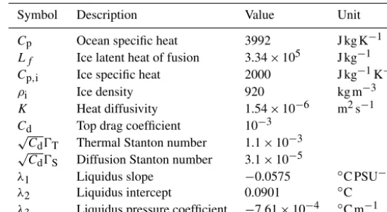
lim-Figure 1.Freshwater and associated latent heat introduced(a)at the surface (R_noISF),(b)beneath the ice shelf (A_ISF, R_ISF and R_MLT),
(c)at the ice shelf base level (A_BG03) and(d)over the depth range of the ice shelf base (A_PAR and R_PAR).
ited extent, the smaller ice shelves nevertheless make a sig-nificant contribution to the total meltwater flux from the ice sheet. We therefore need a way to mimic the impact of unre-solved cavities on the ocean.
Beckmann and Goosse (2003, hereafter BG03) suggested a simple parametrisation for the melting beneath an ice shelf and prescribed the input of meltwater at the ocean level cor-responding to the base of the ice shelf (Fig. 1c). One of the main issues with this parametrisation is that, for the same ice shelf melting, the effect on the ocean dynamics will be the same whatever the grounding line depth is.
The idea tested in this paper is to spread the freshwater due to ice shelf melting evenly between the grounding line depth and the depth of the calving front. In this case, the model cre-ates its own plume along the vertical wall (Fig. 1d, no cavity in this case) and thus an overturning between the grounding line depth and the equilibrium depth (the depth where the density of the plume is equal to the density of the ambient water). Figure 1a and b are discussed in Sect. 5.2.
In this part of the study we focus on how to inject the ob-served ice shelf meltwater flux into the ocean model.
There-fore, the ice shelf melting is prescribed and the heat flux is derived from the freshwater flux using Eq. (8). The compu-tation of the melt rate from the off-shore ocean properties and ice shelf geometry could be included using the BG03 parametrisation or some adaptation of the Jenkins (2011) plume model. The parametrisation tested in this study is kept as simple as possible for ease of use in a wide range of appli-cations. Further testing of other interactive melt parametrisa-tions or fresh water distribuparametrisa-tions that are funcparametrisa-tions of the ice shelf geometry or melt rate is beyond the scope of this study.
3 Academic case
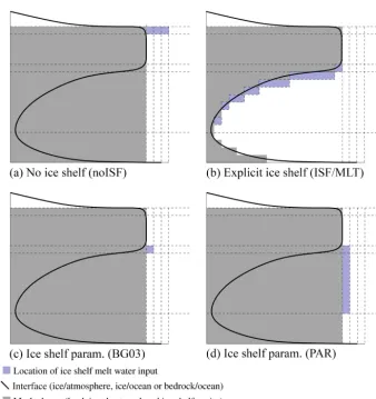
Figure 2. Near-steady-state (after 10 000 days) solution of the I_30M ISOMIP experiment. (a)Horizontal stream function (Psi) in Sv with a contour interval of 0.02 Sv.(b)Meridional overturn-ing circulation (moc) in Sv with a contour interval of 0.01.(c)Melt rate in m yr−1(negative for melting and positive for freezing) with a contour interval of 0.4 m yr−1.
3.1 ISOMIP set-up
The ISOMIP set-up follows the recommendations of the in-ter comparison project for experiment 1.01 (Hunin-ter, 2006). The geometry is based on a closed domain with a flat seabed fixed at 900 m. The grid extends over 15◦in longitude, from 0 to 15◦E with a resolution of 0.3◦, and 10◦in latitude, from 80 to 70◦S with a resolution of 0.1◦. The spatial resolution ranges from 6 km at the southern boundary to 11 km at the northern boundary. The whole domain is covered with an ice shelf, and includes no open-ocean region. The ice shelf draft is uniform in the east–west direction, is set at 200 m between the northern boundary and 76◦S and deepens linearly south of 76◦S down to 700 m at the southern boundary. The water is initially at rest and has a potential temperature of−1.9◦C and a salinity of 34.4 PSU. No restoring is applied to either the temperature and salinity.
The vertical resolution is uniform and fixed at 30 m, al-lowing for a direct comparison with the results of L08. The density is computed using the polyEOS80-bsq function. It takes the same polynomial form as the polyTEOS10 func-tion (Roquet et al., 2015), but the coefficients have been optimized to accurately fit EOS-80 (Fabien Roquet, per-sonal communication, 2015). The melt formulation is the “ISOMIP” one. All the results presented are taken from day 10 000 at which time the system is close to a steady state. 3.2 Model comparison
The ISOMIP experiment has been carried out with many models using different vertical coordinates during the last 10 years, including ROMS1, OzPOM2, MITgcm (Losch, 2008) and POP (Asays-Davis, 2012). All these models agree on a common circulation and melt pattern. The melting and freezing along the base of the ice shelf drives an overturning circulation of about 0.1 Sv. Associated with the meridional overturning circulation, all the models generate a cyclonic gyre with a western boundary current beneath the sloping ice shelf of about 0.3 Sv. This horizontal circulation drives water that is warmer than the freezing point into the south-eastern part of the cavity. The inflow of warm water causes melting at the ice shelf base that is concentrated along the eastern and southern boundaries. On the western side of the ice shelf cavity, the boundary current advects colder water towards the ice front. Shoaling of the ice shelf base causes super-cooling of the water in contact with the ice and thus drives freez-ing. A detailed discussion of this circulation can be found in Grosfeld et al. (1997). The maximum melting–freezing rates are model dependent. The range is 0.7–1.8 m yr−1 for the maximum freezing rate and 0.7–2.4 m yr−1for the maxi-mum melting rate.
The NEMO response to the ISOMIP set-up (simulation I_30M) is shown in Fig. 2. It is similar to that previously
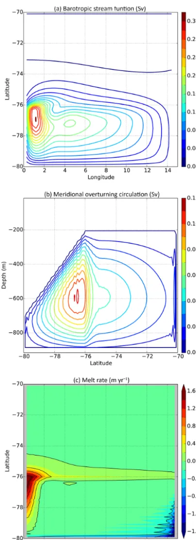
Figure 3. (a) Total melting rate versus total freezing rate, and
(b) meridional overturning circulation versus barotropic stream function (bsf) for all the ISOMIP sensitivity experiments (I_5M, I_10M, I_30M, I_60M, I_100M, I_150M, I_31L, I_46L and I_75L). The simulations I_XXM are with constant vertical resolu-tions of XX m and aHTBLof 30 m, the simulations I_XXMYYM
are with constant vertical resolution of XX m and aHTBLof YY m,
Finally, the simulations I_XXL are with variable vertical resolution. Details are given in Table 2.
simulated with a zcoordinate model (L08). The strength of the overturning circulation is 0.11 Sv. The transport of the western boundary current generated by the cyclonic gyre be-neath the sloping ice shelf is 0.32 Sv. The pattern of melting and freezing is similar to that in L08. The melting occurs, as expected, in the south-eastern corner with a maximum of 2.7 m yr−1 and the freezing takes place beneath the western boundary current with a maximum of 1.9 m yr−1. The low noise is the result of the L08 parametrisation (Fig. 2). In sim-ulations without this parametrisation (not shown) the noise in the melt pattern is as shown in L08.
3.3 Sensitivity of ocean circulation to the vertical resolution
Depending on the scientific question to be addressed, the ocean models commonly used have very different vertical resolutions, ranging from 1 to 100 m. The representation of the top boundary layer is strongly affected by the choice of vertical resolution. To evaluate the impact of this choice on the ocean circulation beneath the ice shelf, nine simulations with vertical resolution ranging from 5 m (I_5M) to 150 m (I_150M) have been carried out (Table 2).
The choice of vertical resolution and LoshHTBLstrongly
affects the ice shelf melting. WhenHTBLis tied to the
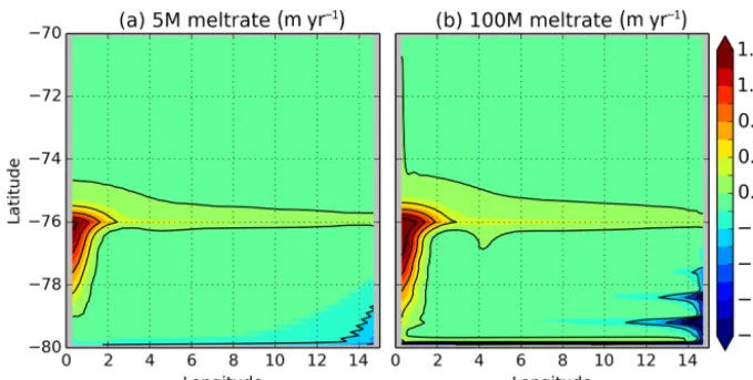
verti-cal resolution, the finer resolution gives lower melting. Under melting conditions, a thin, fresh and cold top boundary layer appears in the top metres of the ocean next to the ice shelf base. With finer vertical resolution, a thinner and colder top boundary layer can be resolved, resulting in weaker melting (Fig. 3a). Our sensitivity experiments show a maximum melt rate 4 times higher in the I_150M simulation (4.3 m yr−1) and 3 times higher in the I_60M simulation (3.1 m yr−1) than in the I_5M simulation (0.9 m yr−1) (not shown). In analogous experiments, L08 found a similar sensitivity, with maximum melting 3 times larger at 45 m resolution than at 10 m res-olution. However, whenHTBL is kept constant (I_5M30M,
I_10M30M and I_30M), the total melt is insensitive to the vertical resolution. The total melt at high vertical resolution (5 or 10 m) with a 30 m Losh top boundary layer thickness (respectively I_5M30M and I_10M30M) is converging to-ward I_30M (Fig. 3a). This suggests that a more physical definition ofHTBL(based on stratification, melt rate, etc . . . ),
rather than a constantHTBL could significantly change the
melt rate in a high-resolution models (although investigation of this is beyond the scope of the paper).
With very coarse resolution (I_100M/I_150M), the model is unable to represent a top boundary layer at all and the total melting saturates. Total melting is 20 % smaller in the I_5M simulation than in both the I_100M and I_150M sim-ulations, which have the same total melt (Fig. 3a). With vari-able vertical resolution (I_31L, I_46L and I_75L), such as is typically used in global configurations of NEMO (Timmer-mann et al., 2005; DRAKKAR group, 2007; Megann et al., 2014), the coarsest resolution in the cavity seems to deter-mine the total melt. This is because more than 50 % of the melting occurs between 500 and 700 m depth where the res-olution is coarsest (not shown). This could be an issue for modelling ice shelf melting with the standard configuration used for climate applications because Dutrieux et al. (2013) show that, for some ice shelves with high melt rates, most of the melt may occur over a small area close to the grounding line, where the resolution is coarsest.
Figure 4.Melt rate in(a)the 5M simulation, and(b)the 100M simulation in m yr−1(negative for melting and positive for freezing) with a contour interval of 0.4 m yr−1.
In contrast, the barotropic stream function and the over-turning circulation in the cavity are not altered by any choice of vertical resolution between 5 and 150 m (Fig. 3b). One of the reasons could be that with the bulk formulation of melt-ing used in the ISOMIP simulations, there is no direct link between the ocean current velocity at the ice-shelf–ocean in-terface and the melt rate, because the thermal exchange coef-ficient is defined to be a constant.
4 Ice shelf cavity parametrisation
While the ice shelf module as described so far works well in idealised cases, for a wider range of applications (includ-ing ice shelves of vary(includ-ing extent at all likely horizontal res-olutions) we also need the capability of representing the im-pact of circulation and melting within unresolved cavities. In this section, we investigate the ability of our ice shelf cav-ity parametrisation to mimic the circulation and water mass properties produced by the full cavity simulation, and com-pare the results with those produced by the parametrisation of BG03. Both parametrisations are evaluated in an idealised configuration derived from the ISOMIP set-up.
The geometry is the one for ISOMIP experiment 2.01, which is the same as that for ISOMIP experiment 1.01 ex-cept in the top 200 m, where the flat ice shelf is replaced by open water (Fig. 5a). The simulations are initialised with a warm linear profile typical of conditions on the continen-tal shelves of the Amundsen and Bellingshausen seas (Fig. 6 in Asay Davis et al., 2016, with constant value between 720 and 900 m). Radiative open boundary conditions are applied at the northern boundary (Treguier et al., 2001). The vertical eddy viscosity and diffusivity, in unstable conditions, is set to 10 m2s−1(instead of 0.1 m2s−1in ISOMIP configuration) to reduce the noise generated along the ice shelf front.
Three experiments are run for 30 years: one with the ice shelf cavity open (A_ISF, Fig. 1b), but with a steady pattern of basal melt/freeze imposed; another with the open-ocean circulation driven by the cavity parametrisation of BG03 (A_BG03, Fig. 1c); and a third with the cavity parametrised as outlined in Sect. 2.3 (A_PAR, Fig. 1d). In all these exper-iments the same heat and freshwater fluxes are applied, de-rived from the basal melt/freeze pattern obtained in the last month of a dedicated 30-year run with explicit ice shelf melt-ing calculated usmelt-ing the “ISOMIP” formulation.
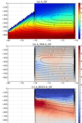
A_ISF drives a deep inflow toward the ice shelf, and cor-responding outflow in the top 400 m toward the open ocean, of 0.9 Sv at the northern boundary (Fig. 5a). In a stratified ocean, this circulation has a crucial effect on the total amount of heat advected toward the ice shelf, on the properties of the water drawn into the overturning circulation and on the overall stratification in the basin. In A_BG03 the overturn-ing is too weak (0.6 Sv compared with 0.9 Sv in A_ISF) and too shallow (200 m compared with 400 m in A_ISF). Conse-quently, the water masses drawn into the overturning come from a different depth and have different T/S properties, and the resulting stratification is too strong, with colder surface waters and warmer deep waters (Fig. 5c). In A_PAR, because the freshwater flux is distributed over the same depth range as in A_ISF (between 200 and 700 m), the vertical extent of the overturning and the water masses drawn in are the same in both A_PAR and A_ISF. The result is a circulation on the shelf that is similar in depth and magnitude and a stratifica-tion that is similar in strength to those simulated in A_ISF (Fig. 5b).
Figure 5. (a)Zonal mean temperature (◦C) after 30 years of the run; in contour, the meridional overturning stream function (Meridional Overturning Circulation, MOC) in the A_ISF experiment.(b)Mean temperature difference (◦C) with respect to A_ISF experiment (A_PAR-A_ISF); in contour, the MOC in the A_PAR experiment.(c)as(b)but for A_BG03.
and the simulation with the open ice shelf cavity should be smaller.
5 Real ocean application
In the ISOMIP test cases, the ocean circulation in the cav-ity compares well with that simulated by other models. Fur-thermore, the suggested parametrisation of ice shelf melting mimics well the circulation and water properties generated by the presence of an open ice shelf cavity. Nevertheless, the bathymetry and ice shelf draft are smooth in these ide-alised cases and the heat transfer coefficient is constant, so the favourable comparison with other models in the idealised
ISOMIP set-up between models as well as the good match between the idealised A_ISF and A_PAR experiment might not be reproduced in a realistic configuration. In the next sec-tion, we assess both the explicit ocean cavity representation and the cavity parametrisation in a realistic circumpolar con-figuration.
5.1 Antarctic configuration set-up
Figure 6.Bathymetry (m) over the Antarctic continental shelf and beneath the ice shelves. Black lines are the cell edges (plotted every 25 cells). The thick grey line is the limit of the Weddell sector of the grid and the thick dashed grey line is the limit of the Ross, Amudsen and Bellingshausen sectors.
Pole, so that the farthest south grid boxes strongly constrain the model time step. To maintain a model time step equal to that used in current global 1/4◦configurations, the Mercator grid is replaced south of 67◦S with two quasi-isotropic bipo-lar grids, one for the Bellingshausen, Amundsen and Ross sea sector and one for the Weddell sea sector (Fig. 6). Each sector is built following the semi-analytical method used to create the tripolar ORCA grid north of 22◦N (Madec and Imbard, 1996). The effective resolution is 13.8 km at 60◦S, increasing to 3.8 km at 86.5◦S, where a pure Mercator grid would have a resolution of 2.2 km. The model uses 75 ver-tical levels with thicknesses varying from 1 m at the surface to 200 at 6000 m depth, giving a vertical resolution ranging from 10 to 150 m beneath the ice shelves. See Sect. 3.3 for the effect of this resolution on ice shelf melting in an ide-alised case.
The bathymetry used for the model domain north of the Antarctic continental shelf is that described by Megann et al., (2014). Over the Antarctic continental shelves the IBCSO dataset (Arndt et al., 2013) is used. The two bathymetry datasets are merged between the 1000 and 2000 m isobath along the Antarctic continental slope. Under the ice shelves, bathymetry (included in the IBCSO dataset) and ice draft are
taken from BEDMAP 2 (Fretwell et al., 2013). The resulting model bathymetry is shown in Fig. 6. Note that for some ice shelves, Fretwell et al. (2013) enforced flotation by lowering the seabed. In addition, we impose a minimum of two verti-cal grid cells within the ocean cavities so that an overturning cell can develop. Where necessary, either the bathymetry or the ice shelf draft, depending on the local configuration, is modified to fit the criterion. If more than one cell has to be modified to fit the water column criterion, the entire water column is masked. Using this procedure, Totten and Dalton (Moscow University in Rignot et al., 2013) ice shelves and the deepest part of Amery Ice Shelf are almost fully masked. Other choices (the momentum advection, tracer advection, diffusion, viscosity, vertical mixing, double diffusion, bottom friction, bottom boundary layer and tidal mixing parametri-sations) are as used in Megann et al. (2014). For the sea ice we use the Louvain-la-Neuve sea-ice model LIM2 (Fichefet and Morales, 1997) with ice rheology based on an elasto-visco-plastic law as described in Bouillon et al. (2013).
model FES 2012 (Carrère et al., 2012). Sea-surface salinity restoring is applied north of 55◦S, river runoff comes from Dai and Trenberth (2002), and iceberg melting based on Rig-not et al. (2013) is evenly distributed at the surface along the Antarctica coast. Ice shelf melt is applied either into the open cavities, at depth following our parametrisation, or as sur-face runoff. The total ice shelf melt in each individual cavity is either interactively computed using the “three equation” formulation or prescribed following the Rignot et al. (2013) estimates.
Radiative boundary conditions are applied at the northern open boundary (Treguier et al., 2001) using velocity, tem-perature and salinity data from a global NEMO ORCA025 simulation (Barnier et al., 2012) forced by the DFS5.2 at-mospheric forcing developed by the DRAKKAR project. To minimise inconsistency, the model is also driven by the same DFS5.2 atmospheric forcing. The methodology ap-plied to build the DFS forcing series is described in Brodeau et al. (2010), and the details of the DFS5.2 are given in a re-port by Dussin et al. (2016). Initial conditions come from the World Ocean Atlas 2013 (Locarnini et al., 2013; Zweng et al., 2013). The model is run for 10 years starting in 1979 and ending in 1988, and the first-order response is investi-gated using output from the last year of the simulation. 5.2 Experiment description
In order to evaluate both the explicit ice shelf module (Sect. 2.2) and the improved parametrisation (Sect. 2.3) in this realistic case, four simulations are run:
– R_noISF: a simulation without ice shelf cavities. Both the ice shelf freshwater flux and the latent heat flux as-sociated with melting of the ice are prescribed at the surface (Fig. 1a).
– R_ISF: a simulation with explicit ice shelf cavities (Fig. 1b), but where both the melt rate of the ice shelves and the latent heat flux at the ice-shelf–ocean interface are specified.
– R_PAR: a simulation without ice shelf cavities (Fig. 1d). Both freshwater and latent heat fluxes from the ice shelves are uniformly distributed along the calv-ing front from its base down to the groundcalv-ing line depth, or the seabed if it is shallower.
– R_MLT: a simulation with explicit ice shelf cavities and interactive melt rates computed by the “three equation” formulation (Fig. 1b).
For R_ISF, R_noISF and R_PAR the same total inputs of freshwater and latent heat are prescribed for each ice shelf and the fluxes are constant over time; only the location of the input changes. The melting pattern used in R_ISF is provided by the simulation R_MLT, while the magnitude is scaled so that the total for each ice shelf matches that from Rignot
et al. (2013). The associated latent heat flux is derived from the melt rate using Eq. (8).
Initially, results from R_noISF and R_ISF are used to eval-uate the sensitivity of the ocean and sea ice properties to the presence of ice shelf cavities in a control set-up with pre-scribed melting. Next, results from R_PAR are compared with those from R_noISF and R_ISF in order to evaluate and validate the ice shelf parametrisation in a realistic case. Fi-nally, results from R_MLT are used to evaluate the modelled ice shelf melting in our circum-Antarctic configuration using the “three equation” ice shelf melting formulation.
5.3 Sensitivity of ocean properties to the ice shelf cavities
In both R_noISF and R_ISF, large-scale open-ocean features are well represented. Simulated ACC transport (135 Sv) and Weddell gyre transport (56 Sv) are similar and compare well with the observations of 137 Sv for the ACC transport (Cun-ningham et al., 2003) and 56 Sv for the Weddell gyre trans-port (Klatt et al., 2005). Temperature and salinity properties north of the continental shelves are also similar in both simu-lations and compare reasonably with WOA2013 (Figs. 7–8). In contrast, the presence of ice shelf cavities in R_ISF sub-stantially affects the ocean properties and dynamics in the coastal Antarctic seas (Figs. 7, 8 and 10).
Over the Bellingshausen and Amundsen seas, the input of freshwater at the surface in R_noISF leads to strong stratifi-cation in the upper 250 m, weak stratifistratifi-cation below (Fig. 9), a weak and shallow vertical circulation (maximum overturn-ing is 0.01 Sv at 70 m depth) and a weak barotropic circu-lation over the continental shelf (Fig. 10). In R_ISF, the in-put of buoyancy at the ice shelf base activates the buoyancy-forced overturning, driving upwelling along the ice-shelf– ocean interface. The overturning circulation entrains 0.23 Sv of a mix of ambient water (CDW) and meltwater along the ice shelf base. This upwelling generates a barotropic circu-lation that follows the f/h contours over the Amundsen and Bellingshausen sea continental shelf (Fig. 10a and c) as ex-plained in Grosfeld et al. (1997). The resulting mixture of CDW and meltwater stabilises at an equilibrium depth be-tween 400 and 60 m (not shown). The upwelling of CDW into the surface mixed layer weakens the thermohaline strat-ification and warms and salinizes the surface layer. These changes in ocean dynamics on the shelf lead to a more re-alistic continental shelf temperature and salinity distribution (Figs. 7–8) and stratification (Fig. 9) in R_ISF compared with R_noISF.
Figure 7.Temperature (◦C) averaged between 300 and 1000 m (year 10, 1988) from(a)R_ISF,(b)R_PAR,(c)R_noISF and(d)World Ocean Atlas 2013 (Locarnini et al., 2013; Zweng et al., 2013).
this paper. In R_noISF, as the overturning is not activated, there is no process to flush the bottom water trapped in the over-deepened basins, so the waters there are not affected by external forcing, and the bottom properties still match the initial conditions after 10 years of the run (Fig. 9).
Over the Ross and Weddell sea continental shelves, the cold, salty HSSW in R_noISF matches the observations and spreads northward across the shelf break toward the open ocean. In R_ISF, the HSSW produced is too fresh (−0.2 PSU, Fig. 8). Weak winds in the atmospheric forc-ing (Dinniman et al., 2015), in addition to a fresher coastal current (Nakayama et al., 2014), the opening of a new path-way for HSSW circulation beneath the ice shelves (Budillon et al., 2003; Nicholls et al., 2009), mixing of HSSW with light surface waters all year long, and a deficiency of the sea-ice model in representing coastal polynyas could all help to explain the absence of HSSW in R_ISF.
5.4 Sensitivity of sea ice properties to the ice shelf cavities
Winter sea ice extent compares well with the 18.3 million km2 estimated from satellite observations (Comiso, 2000) in both R_ISF (18.2 million km2) and
R_noISF (18.4 million km2). The position of the sea-ice edge, being too far south in the Amundsen Sea and too far north in the Weddell Sea and around East Antarctica in both simulations, is not changed significantly by the presence of ice shelf cavities (Fig. 11).
Figure 8.Salinity (PSU) averaged between 300 and 1000 m (year 10, 1988) from(a)R_ISF,(b)R_PAR,(c)R_noISF and(d)World Ocean Atlas 2013 (Locarnini et al., 2013; Zweng et al., 2013).
Figure 9.Profiles (year 10, 1988) in Pine Island Bay in R_noISF (blue), R_ISF (red) and R_PAR (green) of(a)salinity and(b)temperature.
Figure 10.Barotropic stream function (Sv) on the Ross, Amundsen, Bellingshausen and Weddell continental shelves in(a)R_ISF,(b)R_PAR and(c)R_noISF. Stream function isolines out of the±2 Sv range are not plotted.
buoyant overturning along the ice shelf base is smaller, as is the impact on sea ice.
Comparison with spring sea ice thickness estimates de-rived from sea-ice freeboard and snow thickness measure-ments (Fig. 11d; Kurtz and Markus, 2012) shows that sea ice thickness in R_ISF is closer to observation by about 1 m over the warm shelves of West Antarctica. Over the cold shelves, the modelled sea-ice thicknesses are similar in both simula-tions (less than 20 cm differences) and comparable with the observations, which are subject to±40 cm uncertainties.
5.5 Assessment of the simplified ice shelf representation
Figure 11. Mean sea ice thickness (m) from September to November (SON) in colour. Lines represent the sea ice extent (threshold set at 15 % ice concentration) in the observations of Comiso (2000) (grey) and the corresponding simulation (black).(a)R_ISF,(b)R_PAR,
(c)R_noISF and(d)Kurtz and Markus (2012) data. The observational uncertainty is±40 cm.
Over the warm shelves of West Antarctica, R_PAR re-produces well the R_ISF shelf properties and circulation (Figs. 12a and b and 10). Critically, the prescription of the ice shelf meltwater flux at depth drives an overturning cir-culation and spins up the associated gyres within the over-deepened basins. The magnitudes of the gyres are similar between the R_ISF and the R_PAR simulations (Fig. 10b and c). Shelf water properties generated by R_ISF are bet-ter reproduced by R_PAR than by R_noISF over all the West and East Antarctic shelves (Fig. 12a–d). Over the Amund-sen shelf, R_PAR also decreases the stratification and im-proves the mean temperature and salinity profiles compared with R_noISF (Fig. 9).
Over the Ross and Weddell sea shelves, HSSW produced in R_PAR is saltier than in R_ISF (+0.1 PSU). The salinity gradient between the salty western side and the fresher east-ern side of the shelves is larger than in R_ISF (Fig. 12c) and larger than in the observations (Fig. 8). In R_PAR, this is due to the lack of a HSSW circulation pathway beneath the giant Ross (Budillon et al., 2003) and Filchner–Ronne (Nicholls et al., 2009) ice shelves that in reality carries HSSW formed in the west over to the central or eastern shelf. Instead of this
sub-ice shelf circulation that is captured in R_ISF (Fig. 10), R_PAR drives individual gyre circulations within each of the over-deepened basins, similar in structure to, but stronger than, those in R_noISF.
Sea ice extent and thickness in R_PAR match well the R_ISF sea ice characteristics (Fig. 11). Thickness is smaller by more than 1 m in West Antarctica compared with the R_noISF simulation. Around East Antarctica, and over the Ross and Weddell sea shelves, despite the deficiency in rep-resenting the ocean circulation beneath the giant ice shelves, sea ice thickness in R_PAR is similar to that in R_ISF.
reso-Figure 12.Map of temperature in◦C(a, b)and salinity in PSU(c, d)differences between R_PAR and R_ISF(a, c)and R_noISF and R_ISF
(b, d)averaged between 300 and 1000 m.
lution of 1◦cos(θ ), whereθ is the latitude, which is suffi-cient to explicitly represent the two giant ice shelves (L08, Hellmer et al., 2004, 2012).
5.6 Ice shelf melting
In the previous section we showed that specifying a realistic melting pattern at the ice-shelf–ocean interface gives con-vincing results with major improvements in the properties and circulation of the ocean beyond the ice shelves, espe-cially in the Amundsen and Bellingshausen seas. However, prescribing the freshwater flux represents a strong constraint on the range of applications, since the specified fluxes will only be valid for the present oceanic state. To compute melt rates for other oceanic states interactively, and eventually to couple the ocean model to an evolving ice sheet model, re-quires the “three equation” formulation for ice shelf melt-ing. Next, we evaluate the ability of the described circum-Antarctic configuration with the “three equation” ice shelf melting formulation to simulated realistic ice shelf melting.
The total ice shelf melting simulated in R_MLT (1864 Gt yr−1) is slightly above the range of the observa-tional estimate of Rignot et al. (2013) (Table 3). In R_MLT, as in the observations, we can separate the ice shelves into
two different regimes based on the temperature of the wa-ter masses on the continental shelves (Fig. 7d) and the av-erage melt rate: the cold water (Fig. 13b–d) and the warm water (Fig. 13a) ice shelves. As the ice shelf cavity geom-etry is based on recent estimates (Fretwell et al., 2013) and the ice shelf regime modelled in R_MLT are similar to those in recent observations, the modelled ice shelf melt rate are compared with the Rignot et al. (2013) estimates.
5.6.1 Cold water ice shelves
For the Ross, Weddell and East Antarctic continental shelves, the agreement between computed and observed ice shelf melt rates varies. The total melt in R_MLT for these ice shelves (722 Gt yr−1) lies within the range of the observations (475– 867 Gt yr−1) (Table 3). These ice shelves all experience low
melt rates (Fig. 13b–d) due to the presence of cold water on the shelves (Fig. 8).
Table 3.Basal melt in Gt yr−1for the last year of simulation in R_MLT. Observations come from Rignot et al. (2013). Geometry column indicates the main modification to the BEDMAP2 bathymetry/ice shelf draft as follows: GL means the GL is moved seaward, “shallow” means the ice shelf is too shallow away from the grounding line and “narrow” means the narrowest passage into the cavity is one cell wide.
++/+/0/-/– is a summary of the ocean temperature condition at the closest non-extrapolated cell in the WOA2013 observational dataset (Fig. 14).++for ocean temperature differences with regard to WOA2013 of more than 1◦C, +differences in the range 0.5 and 1◦C, 0 differences in the range 0.5 and−0.5◦C, - differences in the range−0.5 and−1◦C and – for ocean temperature differences greater than
−1◦C.
Ice shelf Model Obs Temperature error at the Geometry (Rignot, 2013) ice shelf edge
(observation: WOA2013)
Amery 207 13–59 ++ GL West 26 17–37 0
Shackleton 14 58–88 – GL Ross 111 14–81 0 GL, shallow Larsen C 46 −46–87 0
FRIS 123 111–210 0 GL Brunt+Riiser 39 −6–26 - shallow Fimbul 42 13–43 - GL Cold ice shelves 722 531–1033
Getz 337 131–159 +(east) – (west) shallow Thwaites 74 91–105 +
Pine Island 87 93–109 +
Abbot 52 32–72 +
George VI 298 72–106 + narrow Warm ice shelves 1142 452–630
Others 408 214–425 Total 1864 1263–1737
paths of the main inflows. Large freezing rates occur along the paths of the main outflows that follow the eastern coasts of the Antarctic Peninsula, Berkner Island and Henry Ice Rise. The latter generates a particularly large area of intense freezing in the central part of the ice shelf, north of the ice rises, in agreement with the observation based distributions of Joughin and Padman (2003) and Moholdt et al. (2014).
For Ross Ice Shelf, R_MLT generates a total melt of 111 Gt yr−1, with high melt rates concentrated along the ice front, and lower freezing rates in the central part of the ice shelf (Fig. 13). The total melt is within the range of previous model based estimates (51–260 Gt yr−1) and the melting– freezing pattern is in good agreement with earlier modelling studies (Timmermann et al., 2012; Assmann et al., 2003; Dinniman et al., 2007). However, the total melt simulated in R_MLT is 30 Gt yr−1above the observational range, because
melt rates along the ice front and on the western side of the ice shelf are larger than those inferred from observation (Rig-not et al., 2013; Moholdt et al., 2014).
Total melt of Amery Ice Shelf is overestimated by at least a factor of 5 (Table 3), because the waters on the continen-tal shelf in front of the cavity are warmer than observed by more than 1.2◦C (Fig. 14). As a consequence, the freez-ing within the cavity, evaluated from remote sensfreez-ing and in
situ data (Wen et al., 2010) and simulated by Galton-Fenzi et al. (2012), is absent in R_MLT.
5.6.2 Warm water ice shelves
The ice shelves along the West Antarctic coastline between the Ross and Weddell seas experience a large total melt rate in R_MLT (1142 Gt yr−1) (Fig. 12a), due to the presence of CDW on the continental shelf. This total melt is about twice the recent observation-based estimate (541 Gt yr−1) (Table 3).
The melt rates in R_MLT are realistic for Abbot Ice Shelf (52 Gt yr−1) (Table 3), but slightly underestimated for Thwaites (74 Gt yr−1) and Pine Island Glacier (PIG; 87 Gt yr−1) compared with observation (Table 3). By com-parison with previous modelling studies, R_MLT results for Abbot and PIG ice shelves are in the range of earlier work (Timmermann et al., 2012; Nakayama et al., 2014; Shodlock et al., 2016) while for Thwaites the results are above those obtained previously.
Figure 13.Ice shelf melting (m yr−1, positive values mean melting) in the R_MLT simulation for(a)the West Antarctic ice shelves,(b)Ross Ice Shelf,(c)Filchner–Ronne Ice Shelf and(d)the East Antarctic ice shelves. Note that panels(a)and(b–d)have different colourbars.
et al. (2012) and Nakayama et al. (2014) with RTOPO1 bathymetry (Timmerman et al., 2010), respectively, 164 and 127 Gt yr−1 for Getz Ice shelf, and 86 and 88 Gt yr−1 for George VI Ice Shelf. However, Schodlok et al., (2016) obtained similar melt rates using MITgcm with IBCSO bathymetry (respectively 303.9 and 373.1 Gt yr−1).
These large inter-model differences could have three causes. First, the bathymetry and ice shelf draft data used in Timmermann et al. (2012) and Nakayama et al. (2014) come from RTOPO1, whereas Schodlok et al. (2016) and the present study use bathymetry data from IBCSO and ice shelf draft data from BEDMAP2. Differences in ice shelf geom-etry and bathymgeom-etry, particularly the height of seabed sills, can strongly affect ice-shelf melting (Rydt et al., 2014).
Second, the ability of off-shelf CDW to cross the shelf break and spread across the continental shelf is a key con-trol on the water mass structure within the ice shelf cavities.
In R_MLT (Fig. 14) and MITgcm (Shodlock et al., 2016), CDW flow onto the shelf is well established. However, in the FESOM simulations of Nakayama et al. (2014), the shelf wa-ter is colder than the observations by 0.5 to 3◦C, depending of the horizontal resolution used. Analysis of why CDW can cross the continental shelf break in some models and not in others is beyond of the scope of this paper.
Figure 14.Shown are 300–1000 m mean temperature differences between R_MLT (year 10, 1988) and observations from World Ocean Atlas 2013 (Locarnini et al., 2013; Zweng et al., 2013). Grey area represents ice sheet, ice shelves or ocean shallower than 300 m. The hatched area limited by the green line represents where the observational dataset is obtained by extrapolation.
in Sect. 3.3 show that some ice shelves (West, Dalton, Tot-ten, George VI, Larsen C and FRIS for example) are highly sensitive to the vertical resolution, which affects the ocean properties on the continental shelf, the representation of the top boundary layer beneath the ice shelf, and the ability to resolve details of the cavity geometry.
5.6.3 Limitations
In addition to the inter-model differences described above, ice-shelf–ocean models in general are still subject to several limitations. Most of them are specific to our model set-up as well as the large uncertainties in geometry and forcing data, and critical gaps in our knowledge of dynamics at the ice– ocean interface.
The most recent bathymetry and ice shelf draft recon-struction of the Amundsen Sea (Millan et al., 2017) shows features that are missing in the BEDMAP2 data-set. In BEDMAP2, for many ice shelves, there are only indirect observations of ice draft, based on satellite surface eleva-tion data, while the sub-ice bathymetry data are often poorly constrained. For some ice shelves (Getz, Venable, Stange, Nivlisen, Shackleton, Totten and Dalton ice shelves, some of
the thickest areas of the Filchner, Ronne, Ross and Amery ice shelves and for the ice shelves of Dronning Maud Land), the flotation condition had to be enforced by lowering the seabed arbitrarily from a level that itself was based on nothing more than extrapolation of cavity thickness from surrounding re-gions of grounded ice and 100 m thick cavity. Consequently, more data are needed for effective modelling (Fretwell et al., 2013), because cavity geometry has a major impact on the simulated melting by controlling the water mass structure and circulation within the cavity (Rydt et al., 2014).
Tides have a strong impact on high-frequency variability in melting as well as the magnitude and spatial pattern of the temporal mean melt rate (Makinson et al., 2011), but they are not taken into account in the present study.
Subglacial runoff can enhance melting at the ice–ocean in-terface, especially near the grounding line (Jenkins, 2011). However, the location, magnitude and variability of sub-glacial outflows from beneath the Antarctic Ice Sheet are poorly known (Dierssen et al., 2002; Fricker et al., 2007).
base of an ice shelf of unknown roughness is highly spec-ulative, and the range of values discussed in the literature is wide, ranging from 1.5×10⁻³(Holland and Jenkins, 1999)
to 9.7×10⁻³ (Jenkins et al., 2010), while the basal melt-ing simulated in models is sensitive to the value chosen (Dansereau et al., 2014; Gwyther et al., 2015; Jourdain et al., 2017). Furthermore, the friction law commonly used to com-pute the drag is overly simplistic. The same drag coefficient and friction law are used to compute the stress whatever the dynamic regime appropriate for the grid point location be-neath the ice shelf (i.e. whether it lies within the boundary layer or the free stream flow beyond).
Recent observations beneath George VI ice shelf exhibit thermohaline staircases in the top 20 m below the melting ice shelf base, due to double-diffusive convection (Kimura et al., 2015). These observations raise a doubt about the applica-bility of the widely used three-equation model to predict the melt rate in regions where the flow beneath the ice shelf is weak. More experiments, observations and numerical simu-lations are needed to fully understand the role of turbulence and thermohaline staircases controlling the heat flux to melt-ing ice shelves.
In addition, Dutrieux et al. (2013) suggested that melting can be concentrated around kilometre-scale heterogeneities in ice thickness, such as keels and channels, especially near the grounding line. Furthermore, Stanton et al. (2013), from density measurements in the top 30 m of the ocean beneath Pine Island Glacier, suggest that the top boundary layer can be less than 5 m thick. This means either very high horizontal and vertical resolution or a better melt formulation, or both, are needed to improve the representation of processes near the grounding line and the ice shelf base.
6 Conclusions
An ice shelf capability has been implemented and eval-uated in the NEMO model framework following Losch et al. (2008). The work represents the first step toward a cou-ple ice sheet–ocean model. The working hypothesis used here is that the ice shelf is in equilibrium, with the mass re-moved by melting being replenished by the flow of the ice shelf, so the shape of the sub-ice-shelf cavity remains con-stant over time.
In an idealised case (ISOMIP set-up), the simulated ocean circulation and ice shelf melting are similar to those de-scribed by Losch et al. (2008) using the MITgcm model. Ice shelf melting appears to be sensitive to vertical resolu-tion and top boundary layer definiresolu-tion. When the Losch top boundary layer thickness is fixed, results are independent of vertical resolution and converge toward those obtained with a vertical resolution equal to that of the top boundary layer. When top boundary layer thickness changes with the vertical resolution under melting conditions, models simulate a cold, fresh, top boundary layer that tends to decrease the thermal
forcing and thus the simulated melt rate. At coarse resolu-tion, the cold, top boundary layer is absent, leading to much larger melt rates.
To apply this work to a realistic case, a southward-extended global ORCA grid (eORCA) has been set up us-ing two quasi-isotropic bipolar grids south of 67◦S. The im-pact of including the ice shelf cavities has been evaluated in a circum-Antarctic version of the eORCA grid, by compari-son with a control simulation without ice shelf cavities. The freshwater and heat flux resulting from ice shelf melting is specified at the ice-shelf–ocean interface for the simulation with cavities and at the ocean surface for the control run.
For warm water shelves, prescribing the ice shelf melting at the surface (R_noISF) leads to a stratification that is too strong compared with the observations. With ice shelf cavi-ties included (R_ISF), melting into the cavity drives a buoy-ant overturning circulation and entrains warm and salty CDW into the upwelling branch that subsequently mixes into the cold, fresh surface layers outside of the cavity. The entrain-ment of CDW thus weakens the thermocline by warming and increasing the salinity of the upper ocean layers, resulting in a decrease of the ocean stratification. The activation of the overturning circulation also creates a barotropic circulation that follows f/h contours on the continental shelf.
For cold water shelves, high-salinity shelf water (HSSW) simulated in R_noISF is slightly less dense than observa-tions, but when ice shelf cavities are present, the model is unable to maintain HSSW on the shelf at all. Compared with the simulation without ice shelf cavities, two extra pro-cesses consume the HSSW. The vertical overturning circula-tion driven by melting acts to mix the HSSW with the up-per layers all year long, and the presence of new pathways beneath Ross and Filchner–Ronne ice shelves increases the export of HSSW from its formation location on the western continental shelf. The loss of HSSW with the ice shelf cavity opened is not balanced by increased dense water formation at the surface. This could be a result of deficiencies in any or all of the atmospheric forcing, the sea-ice model used in this study, or the representation of coastal polynyas.
The effects on sea ice are very dependent on the amount of ocean heat available at depth. Over warm water shelves, the CDW entrained into the cavity overturning circulation warms the surface layer all year long and thus restricts the sea ice formation. This warming of the surface layer leads to thinning of the sea ice by more than 1 m in coastal regions of the Bellingshausen and Amundsen seas (2 m locally). Over cold water shelves, including the sub-ice-shelf cavities has a smaller effect on sea ice thickness (less than 20 cm).
coarser resolutions the majority of the freshwater source could be missing.
To mimic the circulation driven by these unresolved ice shelves, the ice shelf melting is uniformly distributed over the depth and width of the unresolved cavity opening, from the mean ice front draft down to the seabed, or the ground-ing line depth if it is shallower. This simple representation of the ice shelf melting drives a buoyant overturning circulation along the coast similar to that would be present within the ice shelf cavity. Idealised and realistic circum-Antarctic experi-ments show that this parametrisation mimics the effect of the overturning circulation within small ice shelf cavities and its impact on water mass properties and circulation on the con-tinental shelf. However, for large ice shelves, such as Ross and Filchner–Ronne, the parametrisation is unable to mimic the effect of the large-scale horizontal ocean circulation be-neath the ice shelf. Thus, the redistribution of meltwater and high-salinity shelf water between the different troughs on the continental shelf via their connections under the ice shelf is missing.
The specification of ice shelf melting, either over the area of the ice shelf base for resolved cavities or over the area of the cavity opening for unresolved cavities, leads to major improvements in the water mass properties, ocean circulation and sea ice state on the Antarctic continental shelf. However, a model that interactively computes ice shelf melting is cru-cial for simulating the ocean and ice sheet response to per-turbations as well as for developing coupled ice-sheet–ocean models. With the parametrised version of the ice shelf pre-sented here, we only explain how to distribute the meltwater fluxes in an ocean model without ice shelf cavities in a phys-ically sensible way. We do not describe a way to compute the melt rate itself. To tackle this issue, this work needs to be combined with a parametrisation of ice shelf melting (for example Beckmann and Goosse, 2003; Jenkins et al., 2011). With the ice shelf cavities opened, the widely-used “three equation” ice shelf melting formulation enables an inter-active computation of melting. The ability of the circum-Antarctic configuration with the “three equation” ice shelf melting formulation to simulated realistic ice shelf melting has been assessed. Comparison with observational estimates of ice shelf melting reported by Rignot et al. (2013) indi-cates realistic results for most ice shelves. However, melting rates for Amery, Getz and George VI ice shelves are consid-erably overestimated and some key ice shelves, such as Tot-ten and Dalton, are missing because of inadequate horizontal and vertical resolution. Possible causes of the overestimated melt rates include poor representation of shelf water prop-erties, inaccurate or poorly resolved cavity shape, unknown ice shelf ocean drag coefficient and poor representation of boundary layer processes.
Despite some deficiencies in the simulation of ice shelf melting and the parametrisation of ocean processes in un-resolved ice shelf cavities, this work is a step forward to-ward a better representation of ice-shelf-ocean interaction in
the NEMO framework for all model resolutions. In practice, for horizontal resolutions finer than 2◦, some of the ice shelf cavities can be resolved (Ross ice shelf for example) while at almost any useable resolution some cavities will have to be parametrised. The most suitable choice of which can be explicitly resolved and which must be parametrised will de-pend on the combination of horizontal and vertical resolution used.
To apply this work to a global coupled ice sheet–ocean model, we will need some further developments. First, a bet-ter knowledge of sub-ice-shelf cavity geometries and key processes that contribute to melting (drag, tides, boundary layer, etc.) could lead to improvements in the ice shelf rep-resentation. Second, parametrisations need to be developed to represent the processes (melt and circulation) where the resolution is not fine enough to represent the ice shelf cavity geometry correctly as at the grounding line for example. Fi-nally, a conservative wetting and drying scheme needs to be developed to allow for the grounding line (and calving front) to move back and forth.
Code and data availability. The model code for NEMO 3.6 is available from the NEMO website (www.nemo-ocean.eu). On reg-istering, individuals can access the FORTRAN code using the open-source subversion software (http://subversion.apache.org/). The branch used for both configurations used in this study is the 2015 development branch named dev_r5151_UKMO_ISF at revi-sion 5204. The ice shelf module is now included in the public NEMO distribution.
The ISOMIP configuration is distributed in NEMO version 3.6 as an unsupported configuration. No file is required to run ISOMIP configuration. For the circum-Antarctic configuration, the input files (cpp keys, namelist, bathymetry, ice shelf draft, iceberg runoff, ini-tial condition, river runoff, tidal mixing and weights for the surface forcings) could be requested from the authors. The surface forcing and the open boundary were provided by the DRAKKAR consor-tium (http://www.drakkar-ocean.eu).
Competing interests. The authors declare that they have no conflict of interest.