https://doi.org/10.5194/gmd-11-915-2018 © Author(s) 2018. This work is distributed under the Creative Commons Attribution 4.0 License.
Modular System for Shelves and Coasts (MOSSCO v1.0) – a flexible
and multi-component framework for coupled coastal ocean
ecosystem modelling
Carsten Lemmen1, Richard Hofmeister1,4, Knut Klingbeil2,a, M. Hassan Nasermoaddeli3,b, Onur Kerimoglu1, Hans Burchard2, Frank Kösters3, and Kai W. Wirtz1
1Institute of Coastal Research, Helmholtz-Zentrum Geesthacht Zentrum für Material- und Küstenforschung, 21502 Geesthacht, Germany
2Department of Physical Oceanography and Instrumentation, Leibniz-Institute for Baltic Sea Research, 18119 Rostock-Warnemünde, Germany
3Section Estuary Systems I, Bundesanstalt für Wasserbau, 22559 Hamburg, Germany
4Institute for Hydrobiology and Fisheries Science, Universität Hamburg, 22767 Hamburg, Germany anow at: Department of Mathematics, University of Hamburg, 20146 Hamburg, Germany
bnow at: Landesbetrieb Straßen, Brücken und Gewässer, Freie und Hansestadt Hamburg, 20097 Hamburg, Germany Correspondence:Carsten Lemmen ([email protected])
Received: 12 June 2017 – Discussion started: 20 June 2017
Revised: 12 January 2018 – Accepted: 30 January 2018 – Published: 12 March 2018
Abstract. Shelf and coastal sea processes extend from the atmosphere through the water column and into the seabed. These processes reflect intimate interactions between physi-cal, chemiphysi-cal, and biological states on multiple scales. As a consequence, coastal system modelling requires a high and flexible degree of process and domain integration; this has so far hardly been achieved by current model systems. The lack of modularity and flexibility in integrated models hin-ders the exchange of data and model components and has his-torically imposed the supremacy of specific physical driver models. We present the Modular System for Shelves and Coasts (MOSSCO; http://www.mossco.de), a novel domain and process coupling system tailored but not limited to the coupling challenges of and applications in the coastal ocean. MOSSCO builds on the Earth System Modeling Framework (ESMF) and on the Framework for Aquatic Biogeochemi-cal Models (FABM). It goes beyond existing technologies by creating a unique level of modularity in both domain and pro-cess coupling, including a clear separation of component and basic model interfaces, flexible scheduling of several tens of models, and facilitation of iterative development at the lab and the station and on the coastal ocean scale. MOSSCO is rich in metadata and its concepts are also applicable out-side the coastal domain. For coastal modelling, it contains
dozens of example coupling configurations and tested set-ups for coupled applications. Thus, MOSSCO addresses the technology needs of a growing marine coastal Earth system community that encompasses very different disciplines, nu-merical tools, and research questions.
1 Introduction
Environmental science and management consider ecosys-tems as their primary subject, i.e. those sysecosys-tems in which the organismic world is fundamentally linked to the physi-cal system surrounding it; there are neither unequivophysi-cally de-fined spatial nor processual boundaries between the compo-nents of an ecosystem (Tansley, 1935). Consequently, holis-tic approaches to ecological research (Margalef, 1963), bio-geochemistry (Vernadsky, 1998, originally 1926), and envi-ronmental science in general (Lovelock and Margulis, 1974) have been called for.
interlinked processes: biological, ecological, physical, and geomorphological, amongst others. Crossing these domain and process boundaries, the dynamics of suspended sedi-ment particles (SPM; see Appendix A for abbreviations), liv-ing particles, and the interaction between water attenuation and phytoplankton growth, for example, are both scientifi-cally challenging and relevant for the ecological state of the coastal system (e.g. Shang et al., 2014; Maerz et al., 2011; Azhikodan and Yokoyama, 2016).
For historical and practical reasons, the representation of the coastal ecosystem in numerical models has been far from holistic. Most often, ecological and biogeochemical processes are described in modules that are tightly cou-pled to one or a few hydrodynamic models. For example, the Pelagic Interactions Scheme for Carbon and Ecosys-tem Studies (PISCES; Aumont et al., 2015) has been inte-grated into the Nucleus for European Modelling of the Ocean (NEMO; Van Pham et al., 2014) and the Regional Ocean Modeling System (ROMS; Jaffrés, 2011). The Biogeochem-ical Flux Model (BFM) has been integrated into the Mas-sachusetts Institute of Technology Global Circulation Model (MITgcm) (Cossarini et al., 2017) and ROMS. These tight couplings not only exclude important processes at the edges of or beyond the pelagic domain, but they also lack flexibility to exchange or to test different process descriptions.
To stimulate the development, application, and interaction of ecological and biogeochemical models independently of a single-host hydrodynamic model, Bruggeman and Bold-ing (2014) presented the Framework for Aquatic Biogeo-chemical Models (FABM), which serves as an intermediate layer between the biogeochemical zero-dimensional process models and the three-dimensional geophysical environment models. FABM has been implemented in the Modular Ocean Model (MOM; Bruggeman and Bolding, 2014), NEMO, the Finite-Volume Coastal Ocean Model (FVCOM; Cazenave et al., 2016), and the General Estuarine Transport Model (GETM; Kerimoglu et al., 2017). With more than 20 bio-geochemical and ecological models included, FABM has en-abled marine ecosystem researchers to describe the system’s many aquatic processes.
The process-oriented modularity realised within FABM, however, lacks the means to describe cross-domain linkages. Historically rooted in atmosphere–ocean circulation models (Manabe, 1969), the coupling of Earth domains is the stan-dard concept in Earth system models (ESMs). Domain cou-pling is also a major challenge in coastal modelling and has been used, for example, in the Coupled Ocean–Atmosphere– Wave–Sediment Transport (COAWST; Warner et al., 2010) system. COAWST is comprised of the Regional Ocean Mod-eling System (ROMS) with a tightly coupled sediment trans-port model, the Advanced Research Weather Research and Forecasting (WRF) atmospheric model, and the Simulating Waves Nearshore (SWAN) wave model. Each of the compo-nents in domain coupling is usually a self-sufficient model that is run in a special “coupled mode”. Interfacing to other
components is done via coupling infrastructure, such as the Flexible Modeling System (FMS; Dunne et al., 2012), the Model Coupling Toolkit (MCT; Warner et al., 2008) and/or the Ocean Atmosphere Sea Ice Soil (OASIS) coupler (Craig et al., 2017), or the Earth System Modeling Framework (ESMF; Theurich et al., 2016; see Jagers, 2010 for an ex-ample intercomparison of coupling technologies). Recently, Pelupessy et al. (2017) introduced the Oceanographic Multi-purpose Software Environment (OMUSE) and demonstrated nested ocean and ocean–wave domain couplings. Their in-tention is to provide a high-level user interface and infras-tructure for coupling existing and new oceanographic mod-els whose spatial representations differ greatly, in particu-lar between Lagrangian- and Eulerian-type representations. The Community Surface Dynamics Modeling System (CS-DMS; Peckham et al., 2013) even allows for the coupling of models implemented in many different languages, as long as all of these describe their capabilities in basic model in-terface (BMI; Peckham et al., 2013) descriptions. Typically, however, only three to five domain components are coupled through one of the above technologies (Alexander and East-erbrook, 2015).
The differentiation between domain and process coupling is not a technical necessity: a typical domain coupling soft-ware like ESMF can also be used to couple processes. With the Modeling Analysis and Prediction Layer (MAPL; Suarez et al., 2007), the Goddard Earth Observing System version 5 (GEOS-5) encompasses 39 process models coupled hierar-chically through ESMF. The development of these modules, however, is strictly regulated within the developing labora-tory. Vice versa, a typical process coupling infrastructure like the Modular Earth Submodel System (MESSy; Jöckel et al., 2005), which initially linked mostly atmospheric processes, has been generalised to support linking at a user-chosen gran-ularity regardless of the process versus domain dichotomy (e.g. Kerkweg and Jöckel, 2012).
2 MOSSCO concepts
The modularity and coupling concepts proposed in this paper describe a novel software system that addresses the needs of researchers who want to make maximum use of their existing knowledge in a specific field (e.g. geomorphology or marine ecology) but wish to conduct integrative research in a wider and flexible context. In strengthening the independence from specific physical drivers, the new concept should, in addition to addressing the problems listed above, support (1) liaisons between traditionally separated modelling communities (e.g. coastal engineers, physical oceanographers, and biologists), (2) intercomparison studies of physical, geological, and bio-logical modules, and (3) up-scaling studies in which models developed on the laboratory scale in a non-dimensional con-text are applied to regional, global, and Earth system scales.
The design of MOSSCO is application oriented and driven by the demands for enabling and improving integrated re-gional coastal modelling. It is targeted towards building cou-pled systems that support decision making for local poli-cies implementing the European Union Water Framework Directive (WFD) and Marine Strategic Planning Directive (MSPD). From a design point of view we envisioned a sys-tem that is foremost flexible and equitable.
Flexibility means that the system itself is able to deal on the one hand with a diverse small or large constellation of coupled model components and on the other hand with different orders of magnitude of spatial and temporal resolutions; it is able to deal equally well with zero-, one-zero-, two-zero-, and three-dimensional representations of the coastal system. Flexibility implies the capability to also encapsulate existing legacy models to create one or more different “ecosystems” of models. This feature should allow for the seamless replacement of individual model components, which is an important procedure in the continual development of integrated systems. Flex-ibly in replacing components finally creates a test bed for model intercomparison studies.
Equitability means that all models in the coupled frame-work are treated as equally important and that none is more important than any other. This principle dissolves the primacy of the hydrodynamic or atmospheric mod-els as the central hub in a coupled system. Also, data components are as important as process components or model output; any de facto difference in model impor-tance should be grounded in the research question and not on technological legacy. As complexity grows by coupling more and more models, this equitability also demands that experts in one particular model can rely on the functionality of other components in the system without having to be an expert in those models as well. The equitability design extends to participation: contri-butions to the development of components or the coupling
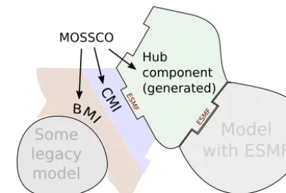
Figure 1.MOSSCO’s adoption of legacy code follows the two-layer paradigm of BMI–CMI (basic model interface–component model interface) suggested by Peckham et al. (2013). An existing legacy code (illustrated by “some model”) is enhanced by model-specific code that exhibits basic coupling functionality (BMI) and is frame-work agnostic. In a second step, a component (CMI) is added that uses the BMI in the specific application programming interface of the coupling framework. In addition to model interfaces that can be used in MOSSCO-independent contexts, MOSSCO provides cou-pling concepts and working implementations for coupled applica-tions.
framework itself is allowed and encouraged. Anyone can use and modify the coupled framework or parts of both in a legal sense through open source licencing and in an accessibility sense through template codes and extensive documentation. 2.1 Wrapping legacy models – first steps inPARSE
As MOSSCO is built around the ESMF hierarchy of compo-nents, any existing code that can be wrapped in an ESMF component can be a component in MOSSCO, too. The ESMF user guide (ESMF Joint Specification Team, 2013) suggests a best practice method,PARSE, to achieve this com-ponentisation of a legacy code.
P repare the user code by splitting it into three phases that initialise, run, and finalise a model.
A dapt the model data structures by wrapping them in ESMF infrastructure like states and fields.
R egister the user’s initialise, run, and finalise routines through ESMF.
S chedule data exchange between components.
E xecute a user application by calling it from an ESMF driver.
the code is independent of the use of ESMF and provides the basic coupling ability – or “coupleability” – of the model; many existing models already implement this separation into initialise, run, and finalise phases, either structurally or more formally by implementing a BMI. For the run phase, it is mandatory to refer to a single model timestep and not to the entire run loop.
The adaption of a model’s internal structures to ESMF
consists of technically wrapping data into ESMF commu-nication objects and providing sufficient metadata for com-munication. Among these are the grid definition and decom-position, units, and semantics of data, optimally following a metadata scheme like the widespread Climate and Fore-cast (CF; Eaton et al., 2011) or the more bottom-up Com-munity Surface Dynamics Modeling System (CSDMS; fol-lowing a scheme like object+operation+quantity; Peck-ham, 2014). Both are currently being included in the emerg-ing Geoscience Standard Names Ontology (GSN; http:// geoscienceontology.org).
ESMF provides the interfaces for models written in ei-ther the Fortran or C programming languages; data arrays are bundled together with related metadata in ESMF field objects. All field objects from components are then bundled into exported and imported ESMF state objects to be passed between components. As a third step, the ESMF registra-tion facility, needs to be added to a user model; this step is achieved by using template code from any one of the exam-ples or tutorials provided with ESMF. The second and third step (adaptandregister) are typical tasks of what Peckham et al. (2013) refer to as a component model interface (CMI); it is very similar between models (and thus easily accessi-ble from template code) and targets the interface of a specific coupling framework.
MOSSCO contains CMIs for ESMF in all of its provided components (Fig. 1). The current naming scheme follows the CF convention for standard names except for quantities that are not defined by CF; these names (often from biological processes) are modelled onto existing CF standard names as much as possible. MOSSCO also allows for specification within other naming schemes and includes a name-matching algorithm to mediate between different schemes. For future development, adoption of the GSN ontology is foreseen. 2.2 Scheduling in a coupled system – the “S” inPARSE
MOSSCO adds onto ESMF a scheduling system (corre-sponding to the fourth step inPARSE) that calls the different phases of participating coupled models. The coupling time step duration of this new scheduler relies on the ESMF con-cept of alarms and a user specification of pairwise coupling intervals between models. The scheduler minimises calls to participating models by flexibly adjusting time step duration to the greatest common denominator of coupling intervals pertinent to each coupled model. Upon reading the user’s coupling specification, (i) models are initialised in random
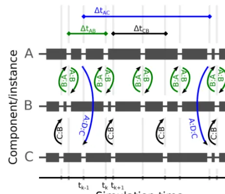
Figure 2.Scheduling of three coupled component instances A, B, C and their data exchanges according to a pairwise coupling speci-fication (see Fig. 3b); shown along a simulation time axis, which is independent of the type of (sequential or concurrent) deploy-ment. Note how each individual component instance has varying run lengths resulting from the interference of all coupling intervals with this component. The time steps of the (anonymous) scheduler componenttk+n(grey bars) vary according to the interference
pat-tern of all coupling intervals. Coupling specification (Fig. 3): A cou-ples bidirectionally to B at interval1tAB(green), A couples
unidi-rectionally to C via a coupler D at interval1tAC(blue), C couples
unidirectionally to B at interval1tCB(black).
order but with consideration of special initialisation depen-dencies set by the user; (ii) a list of alarm clocks is generated that considers all pairwise couplings a model is involved in; (iii) special couplers associated with a pairwise coupling are executed; (iv) the scheduler then tells each model to run until that model reaches its next alarm time; and (v) the advanc-ing of the scheduler to the minimum next alarm time repeats until the end of the simulation.
The MOSSCO scheduler allows for both sequential and concurrent coupling of model components or a hybrid cou-pling mode. In the concurrent mode, components run at the same time on different computing resources; in the sequen-tial mode, components are executed one after another on the same set of computing resources. Recently, Balaji et al. (2016) demonstrated how a hybrid coupling mode and fine granularity could be used to increase the performance of a system that consists of both highly scalable and less scalable components. In their system, an ocean and an atmosphere component run concurrently; within the atmospheric compo-nent, the radiation code is executed concurrently to a com-posite component that encompasses a sequential coupling of all non-radiative atmospheric processes.
the connectors and mediator components that exchange the data before the components are run. For sequential mode, the coupling configuration also allows for a memory efficient scheme in which consecutive components operate on shared data that always reflect the most recently calculated data from the previous component (Fig. 2; see also Sect. 3.3.1); such se-quential coupling on shared data potentially introduces mass imbalances.
Users specify the coupling in a text format using YAML (short for YAML Ain’t Markup Language; http://yaml.org) notation, a human-reader-friendly data serialisation standard. The itemcouplingcontains a list ofcomponentsthat it-self contains a list of coupled components; in the simple ex-ample (Fig. 3a) two components named “A” and “B” are cou-pled. By default, these components are coupled in sequential mode with the default connector sharing their data; the exe-cution order of A and B is not specified. In a more elaborate example (Fig. 3b), the order of components in the scheduler is specified in thedependencysection, indicating a run se-quence of first A, then B, and last C; all components run on the same set of computing resources in (default) sequential coupling mode.
The instances section declares that the component named C is an instance (or copy) of A; this makes it possible to reuse components multiple times in (possibly different) configurations. Typically, data reader or writer components are instantiated from a generic input–output component to access different files for model input and output. Multiple couplings between the three components A, B, and C are present with couplingintervals that lead to the schedul-ing of couplschedul-ing events accordschedul-ing to Fig. 2. Between A and C, a special coupler “D” handles the data exchange instead of the default connector.
2.3 Deployment of the coupled system – the “E” in
PARSE
MOSSCO provides a Python-based generator that dynam-ically creates an ESMF driver component in a star topol-ogy that then acts as the scheduler for the coupled system. This generator reads the specification of pairwise couplings (Fig. 3) and generates a Fortran source file that represents the scheduler component. The generator takes care of compila-tion dependencies of the coupled models and of coupling de-pendencies, such as grid inheritance; in addition to the basic init–run–finalise BMI scheme, it also honours multi-phase initialisation (as in the National Unified Operational Pre-diction Capability, NUOPC, ESMF extension) and a restart phase. The generated code structurally and functionally re-sembles a NUOPC driver, but it does not require implemen-tation of the NUOPC extension, which is currently restricted to handling only structured grid-based sub-models.
A MOSSCO command line utility provides a user-friendly interface to generating the scheduler, (re-)compiling all source codes into an executable and submitting the
exe-cutable to a multi-processor system, including different high-performance computing (HPC) queueing implementations; this is the fifth step in PARSE. By designing this com-mand line utility and automatic scheduler component cre-ation based on the simple YAML textual coupling specifica-tion, MOSSCO provides a fast way to reconfigure, rearrange, extend, or reduce coupled systems very quickly in contrast to more elaborate graphical coupling tools such as the CUPID Eclipse interface (Dunlap, 2013, only for NUOPC).
MOSSCO has been successfully deployed at several na-tional HPC centres, such as the Norddeutsche Verbund für Hoch- und Höchstleistungsrechnen (HLRN), the German Climate Computing Center (DKRZ), and the Jülich Super-computing Centre (JSC). Equally, MOSSCO is currently functioning on a multitude of Linux and macOS laptops, desktops, and multiprocessor workstations using the same MOSSCO (bash-based) command line utility on all plat-forms.
The MOSSCO coupling layer is coded in Fortran, while most of the supporting structure is coded in Python and par-tially in bash syntax. The system requirements are a For-tran 2003 compliant compiler, the CMake build system, the Git distributed version control system, Python with YAML support (version 2.6 or greater), a Network Common Data Form (NetCDF; Rew and Davis, 1990) library, and ESMF (version 7 or greater). For parallel applications, a message-passing library (e.g. OpenMPI) is required. Many HPC cen-tres have toolchains available that already meet all of these requirements. For an individual user installation, all require-ments can be taken care of with one of the package man-agers distributed with the operating system, except for the installation of ESMF, which needs to be manually installed; MOSSCO provides a semi-automated tool for helping in this installation of ESMF. The steps to get MOSSCO run-ning quickly on any suitable computer system are outlined in Fig. 3c. These instructions should get a reader started on car-rying out initial simulations with a coupled system by typing a dozen lines of code, provided that all requirements are met.
3 MOSSCO components and utilities
Driven by user needs, MOSSCO currently entails utilities for I/O, an extensive model library, and coupling functional-ities (Fig. 4 and Table 1). As a utility layer on top of ESMF, MOSSCO also extends the application programming inter-face (API) of ESMF by providing convenience methods to facilitate the handling of time, metadata (attributes), configu-ration, and to unify the provisioning and transfer of scientific data across the coupling framework. The use of this utility layer is not mandatory; any ESMF-based component can be coupled to the MOSSCO-provided components without us-ing this utility layer.
# This YAML text file specifies # a minimal coupling for MOSSCO # using only two components # and default couplers/intervals
coupling:
components: - A - B
# This YAML text file specifies # a more elaborate coupling for MOSSCO # using three components and two couplers
dependencies:
- B: A # run B after A
- C: B # run C after B
instances:
- C: A # run C as instance of A
coupling:
- components:
- A # send component
- B # receive component
interval: 10 h # Dt_AB in Fig. 2
- components: - B - A
interval: 10 h - components: - C - B
interval: 14 h # Dt_CB in Fig. 2
- components: - A
- D # this is the coupler
- C
interval: 34 h # Dt_AC in Fig. 2
(a)
(b)
(c)
#! /bin/bash
export MOSSCO_DIR=$HOME/MOSSCO/code
export MOSSCO_SETUPDIR=$HOME/MOSSCO/setups
export NETCDF=NETCDF4
git clone --depth=1 git://git.code.sf.net/p/mossco/code $MOSSCO_DIR git clone --depth=1 git://git.code.sf.net/p/mossco/setups $MOSSCO_SETUPDIR
make −C $MOSSCO_DIR external # download external codes
mkdir −p $HOME/opt/bin
export PATH=$PATH:$HOME/opt/bin
ln −sf $MOSSCO_DIR/scripts/mossco.sh $HOME/opt/bin/mossco # "installation"
cd $MOSSCO_SETUPDIR/helgoland # choose a Helgoland 1D setup
mossco jfs # starts a 1D pelagic−sediment simulation 1
2 3
4 5
6
7 8 9
10 11
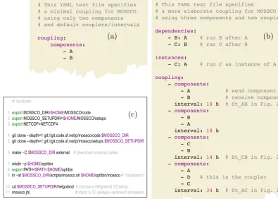
Figure 3.Examples of coupling configurations(a, b)and the steps from installation to deployment(c). The configurations exhibit a minimal
default coupling specification (a)and a more complex one (b, see Fig. 2) that makes use of dependencies, instantiation, and different
coupling intervals. The line-numbered installation steps(c)include environment variable specification (export), download of the system
with git, loading additional external models withmake, installation of themosscoexecutable script, and finally deployment of the
coupling specificationjfsin a predefined set-up called “helgoland”, a 1-D station near the island of Helgoland in the southern North Sea.
Table 1.Components currently integrated into MOSSCO and described shortly in this paper. Several other components are under develop-ment and not listed here.
Pelagic ecosystem fabm_pelagic_component Sect. 3.1.1
Soil ecosystem fabm_sediment_component Sect. 3.1.2
1-D hydrodynamics gotm_component Sect. 3.1.3
3-D hydrodynamics getm_component Sect. 3.1.4
Filtration filtration_component Sect. 3.1.6
Erosion and sedimentation erosed_component Sect. 3.1.5
Wind waves simplewave_component Sect. 3.1.7
NetCDF output netcdf_component Sect. 3.2.1
NetCDF input netcdf_input_component Sect. 3.2.2
Link connector link_connector Sect. 3.3.1
Copy connector copy_connector Sect. 3.3.1
Nudge connector nudge_connector Sect. 3.3.1
Tracer transport transport_connector Sect. 3.3.2
Benthic–pelagic coupling soil_pelagic_connector pelagic_soil_connector Sect. 3.3.3
spatial representations, while maintaining the coupling con-figuration to the maximum extent possible. This design prin-ciple builds on the dimensional independency concept of FABM achieved by the local description of processes (of-ten referred to as a box model), in which the
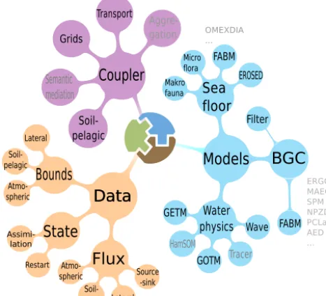
Figure 4.Modular components of MOSSCO. The blue branch col-lects newly created sub-models and components that wrap around legacy codes; the violet branch collects coupling functionalities and the orange branch the input–output utilities.
transect (two-dimensional) and a full atmosphere or ocean (three-dimensional) set-up. As a concrete example, the novel Model for Adaptive Ecosystems in Coastal Seas (MAECS; Wirtz and Kerimoglu, 2016; Kerimoglu et al., 2017) has been developed, iterating between an application for the lab (zero-dimensional) scale and the three-dimensional regional coastal ocean scale.
All utility functions and components, especially the model-independent I/O facilities from MOSSCO, are able to handle data of any spatial dimension. Components that do not define their own spatial representation as a grid or mesh are able to inherit the complete spatial information from a coupled component that provides such a grid: usually (but not necessarily) biological and chemical models inherit the spatial configuration from a hydrodynamic model. Equally, this information can be obtained from data in standardised grid description formats like Gridspec (Balaji et al., 2007) or the Spherical Coordinate Remapping and Interpolation Pack-age (SCRIP; Jones, 1999). Grid inheritance is specified as a dependency in the coupling specification.
3.1 Model library: model interfaces for scientific model components
The model library (right branch in Fig. 4) includes new mod-els (e.g. for filter feeders and surface waves) and wrappers to legacy models and frameworks such as FABM or GETM. Some of these wrappers are under development, among them the Hamburg Shelf Ocean Model (HamSOM; Harms, 1997) and a Lagrangian particle tracer model. Here, we briefly
doc-ument the model collection, particularly with respect to their preparation and functioning within the new coupling context.
3.1.1 Pelagic ecosystem component
The pelagic ecosystem component
(fabm_pelagic_component) collects (mostly bio-logical) process models for aquatic systems. This component makes use of the Framework for Aquatic Biogeochemical Models (Bruggeman and Bolding, 2014). FABM is a coupling layer to a multitude of biogeochemical models which provide the source-minus-sink terms for variables, their vertical local movement (e.g. due to sinking or ac-tive mobility), and diagnostic data. Each model variable is equipped with metadata, which is transferred by the ecosystem component into ESMF field names and attributes. Similarly, the forcing required by the biogeochemical models is communicated within the framework and linked to FABM. The pelagic ecosystem component includes a numerical integrator for the boundary fluxes and local state variable dynamics. Advective and diffusive transport are not part of this component but are left to the hydrodynamical model through thetransport_connector(Sect. 3.3.2). The close connection between transport and the pelagic ecosystem requires that the spatial representation of the FABM state variables be inherited from the hydrodynamic model component that performs the transport calculations.
Many well-known biogeochemical process models have been coded in the FABM standard by various institutes, such as the European Regional Seas Ecosystem Model (ERSEM; Butenschön et al., 2016), ERGOM (Hinners et al., 2015), PCLake (Hu et al., 2016), and the Bottom RedOx Model (BROM; Yakushev et al., 2017). All pelagic biogeochemi-cal models complying with the FABM standard can equally be used in MOSSCO, while retaining their functionality. 3.1.2 Sediment and soil component
pore water as part of the bulk sediment, while all state vari-ables are measured per volume of pore water in each cell. The FABM infrastructure of state variable properties is used to label the new boolean propertyparticulatein FABM models to define whether a state variable belongs to the solid phase within the domain. A typical model used in appli-cations of the sediment component is the biogeochemical model of the Ocean Margin Exchange Experiment OMEX-DIA (Soetaert et al., 1996); a version of this model with added phosphorous cycle is contained in the FABM model library as OMEXDIA_P (Hofmeister et al., 2014).
3.1.3 1-D Hydrodynamics: General Ocean Turbulence Model (GOTM))
The General Ocean Turbulence Model (GOTM; Burchard et al., 1999, 2006) is a one-dimensional water column model for hydrodynamic and thermodynamic processes re-lated to vertical mixing. MOSSCO provides a component for GOTM and a component hierarchy that considers a coupled GOTM with internally coupled FABM within one compo-nent (gotm_fabm_component), as many existing avail-able model set-ups rely on the direct coupling of FABM to GOTM. This way, the modularisation – taking a cou-pled GOTM–FABM apart and recoupling it through the MOSSCO infrastructure – can be verified; the encapsulation of GOTM is implemented in thegotm_component. 3.1.4 3-D Hydrodynamics: General Estuarine
Transport Model (GETM)
MOSSCO provides an interface to the 3-D coastal ocean model GETM (Burchard and Bolding, 2002). GETM solves the Navier–Stokes equations under Boussinesq approxima-tion, optionally including the non-hydrostatic pressure con-tribution (Klingbeil and Burchard, 2013). A direct interface to GOTM (see Sect. 3.1.3) provides state-of-the-art turbu-lence closure in the vertical. GETM supports horizontally curvilinear and vertically adaptive meshes (Hofmeister et al., 2010; Gräwe et al., 2015). The interface to GETM is pro-vided by the getm_component; any model coupled to GETM via the transport component can have its state vari-ables conservatively transported by GETM (see Sect. 3.3.2). In the component, the GETM-created spatial topology is made available as an ESMF grid object; typically this grid and subdomain decomposition is communicated to the cou-pled system in which the spatial and parallelisation informa-tion is inherited by other components.
3.1.5 Model components for erosion, sedimentation, and their biological alteration
The erosion and sedimentation routines of the Deltares Delft3D model (EROSED; van Rijn, 2007) were en-capsulated in a MOSSCO component. EROSED uses a Partheniades–Krone equation (Partheniades, 1965) for
cal-culating the net sediment flux of cohesive sediment at the water–sediment interface for multiple SPM size classes. The MOSSCO BMI uses the current version of EROSED maintained by Deltares; it isolates with the help of sub-sidiary infrastructure the original code from the deeply intertwined dependencies in the Delft3D system. The erosed_componentcan provide its own spatial represen-tation as a structured grid or unstructured mesh; it can also in-herit the spatial information from a coupled component. The functionality of the erosion and sedimentation component is described in more detail by Nasermoaddeli et al. (2014).
Flow and sediment transport can be affected by the pres-ence of benthic organisms in many ways. Protrusion of ben-thic animals and macrophytes in the boundary layer changes the bed roughness and thus the bed shear stress and conse-quently the sediment transport. The erodibility of sediment can be modified by the mucus produced by benthic organ-isms; the erodibility of the upper bed sediment can be altered by bioturbation generated by macrofauna (de Deckere et al., 2001). In thebenthos_component, these biological ef-fects of microphytobenthos and of benthic macrofauna on sediment erodibility and critical bed shear stress are param-eterised and provided to other coupled components (e.g. the erosion and sedimentation component) as additional erodi-bility and critical shear stress factors. The benthos effect model is described in detail by Nasermoaddeli et al. (2018). 3.1.6 Filter feeding model
The filtration_component describes the instanta-neous filtration by suspension feeders within the water col-umn. This biological filtration model follows Bayne et al. (1993) and describes the filtration rate as a function of food supply; it can be adapted to different species of fil-ter feeders and was recently applied to describing the ecosystem effect of blue mussels on offshore wind farms as the filtration_component of MOSSCO (Slavik et al., 2018). The filtration model uses an arbitrary chemi-cal species or compound, for example phytoplankton carbon, as the “currency” for processing. The ambient phytoplank-ton carbon concentration is sensed by the model organisms and filtered along with the other nutrients (in stoichiomet-ric proportion) out of the environment, creating a sink term for subsequent numerical integration in the pelagic ecologi-cal model.
3.1.7 Wind waves
bot-tom stresses. Coupling to 3-D ocean models and the calcula-tion of addicalcula-tional wave-induced momentum forces, follow-ing either the radiation stress or vortex force formulation (Moghimi et al., 2013), is possible as well. For the inclusion of wave–wave or wave–current interactions in realistic 3-D applications, coupling to a more advanced third-generation wind wave model like SWAN, WaveWatch III, or a wave at-mospheric model (WAM) would be necessary.
3.2 Input–output utilities
The input and output (I/O) utilities include general purpose coupling functionalities that deal with boundary conditions, provide a restart facility, and add surface, lateral, and point source fluxes (lower left branch in Fig. 4).
3.2.1 NetCDF output
This component of MOSSCO provides an output facility netcdf_componentfor any data that are communicated in the coupling framework. The component writes one- to three-dimensional time-sliced data into a NetCDF (Rew and Davis, 1990) file and adds metadata on the simulation to this output. Multiple instances of this component can be used within a simulation such that output of different variables, differently processed data, and output at various time steps can be recorded. The output component is fully parallelised with a grid decomposition inherited from one of the coupled science or data components. In order to reduce interprocess communication during runtime, each write process considers only the part of the data (its data tile) that resides within its computing domain. This comes at a cost to the user, who has to post-process the output tiles to combine for later analysis; a Python script is provided with MOSSCO that takes care of joining tiled files.
The output component also adds metadata that is collected from the system and the user environment at the creation time of the output files. Diagnostics on the processing element and run time between output steps are recorded. The structure of the NetCDF output follows the Climate and Forecast (CF; Eaton et al., 2011) convention for physical variables, geolo-cation, units, dimensions, and methods modifying variables. When (mostly biological) terms are not available in the con-trolled vocabulary of CF, names are built to resemble those contained in the standard.
3.2.2 NetCDF input
The netcdf_input_component of MOSSCO reads from NetCDF files and provides the file content wrapped in ESMF data structures (fields) to the coupling framework. It inherits its decomposition from other components in the cou-pled system. Data can be read from a single file for the entire domain or from distributed files for all decomposed comput-ing elements separately. Upon readcomput-ing data, fields can be
re-named and filtered before they are passed on to the coupled system.
The input component is typically used to initialise other components for restarting, to provide boundary conditions, and for assimilating data into the coupled system. The input facility supports the interpolation of data in time upon read-ing the data with nearest, most recent, and linear interpola-tion. It also supports reading climatological data and trans-lates the climatological time stamp to a simulation present time stamp in the coupling framework.
3.3 MOSSCO connectors and mediators
Information in the form of ESMF states that contain the output fields of every component are communicated to the ESMF driver; requests for data by every component are also communicated to the ESMF driver component. MOSSCO connectors are separate components that link the output and requested fields between pairwise coupled components. MOSSCO informally distinguishes between connector com-ponents that do not manipulate the field data on transfer at all (or only slightly) and mediator components that extract and compute new data out of the input data.
3.3.1 Link, copy, and nudge connectors
The simplest and default connecting action between compo-nents is to share a reference (i.e. a link) to a single field that resides in memory and can be manipulated by each compo-nent; in contrast, thecopy_connectorduplicates a field at coupling time. The consideration of a link or copy connec-tor is important for managing the data flow sequence in a cou-pled system: the copy mechanism ensures that two coucou-pled components work on the same lagged state of data, whereas the link mechanism ensures that each component works on the most recent data available.
Thenudge_connector is used to consolidate output from two components through the weighted averaging of the connected fields. It is typically used as a simple assimilation tool to drive model states towards observed states or to im-pose boundary conditions.
These connectors can only be applied between compo-nents that run on the same grid (but maybe with a dif-ferent subdomain decomposition). Thelink_connector can only be applied between components with an identical subdomain decomposition so that the components have ac-cess to the same memory. Components on different grids re-quire regridding, which is currently under development in MOSSCO.
3.3.2 Transport connector
transport_connector collects state variables to be transported from any coupled component and communicates this collection to the hydrodynamic component based on the availability of both the tracer concentrations and their rate of vertical movement independent of the water currents. This connector is usually called only once per coupled pair of components during the initialisation phase.
3.3.3 Mediators for soil–pelagic coupling
One aspect of the generalised coupling infrastructure in MOSSCO is the use of connecting components that medi-ate between technically or scientifically incompatible data field collections. The soil–pelagic coupling of biogeochemi-cal model components with a variety of different state vari-ables raises the need for these mediators. The use of media-tors leaves the level of data aggregation, data disaggregation, and unit conversion to the coupling routine instead of requir-ing specific output from a model component dependrequir-ing on its coupling partner component.
For soil–pelagic (or benthic–pelagic) coupling, the soil_pelagic_connector mediates the soil biogeo-chemistry output towards the pelagic ecosystem input and the pelagic_soil_connector mediates the pelagic ecosystem output towards the soil biogeochemistry input. Examples include the following: (i) disaggregation of solved inorganic nitrogen to dissolved ammonium and dis-solved nitrate; (ii) filling missing pelagic state fields for phos-phate using the Redfield equivalent for dissolved inorganic nitrogen; and (iii) calculation of the vertical flux of par-ticulate organic matter (POM) from the water column into the sediment depending on POM concentrations in the near-bottom water, its sinking velocity, and a sedimentation effi-ciency depending on the near-bottom turbulence. The effec-tive vertical flux is communicated into the pelagic ecosys-tem component to budget the respective loss and is commu-nicated to the soil biogeochemistry component to account for the respective new mass of POM. The mediator also handles (iv) disaggregation of a single oxygen concentration (allow-ing for positive and negative values) into dissolved oxygen concentration, if positive, and dissolved reduced substances, if negative, and (v) aggregation of pelagic POM composition (variable nitrogen to carbon ratio) into fixed stoichiometry POM pools in the soil biogeochemistry.
4 Selected applications as feasibility tests and use cases MOSSCO was designed for enhancing flexibility and equi-tability in environmental data and model coupling. These de-sign goals have been helpful in generating new integrated models for coastal research with applications at different marine stations (1-D), transects (2-D), and sea domains (3-D). Below, we describe from a user perspective the added value and success of the design goals obtained from using
MOSSCO in selected applications; here, the focus is not on the scientific outcome of the application (these are described elsewhere by Nasermoaddeli et al., 2018, Slavik et al., 2018, and Kerimoglu et al., 2017). All set-ups described in the use cases are available as open source (with limited forcing data due to space and bandwidth constraints).
4.1 Helgoland station
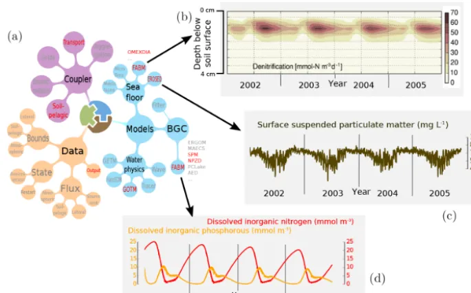
The seasonal dynamics of nutrients and turbidity emerge from the interaction of physical, ecological, and biogeo-chemical processes in the water column and the underlying sea floor. We resolve these dynamics in a coupled application for a 1-D vertical water column for a station near the German offshore island of Helgoland. Average water depth around the island is 25 m; tidal currents are affected by the M2 and S2 tides with a characteristic spring–neap cycle, with current velocity not exceeding 1 m s−1.
The Helgoland 1-D application is realised by a cou-pled system consisting of GOTM hydrodynamics, the pelagic FABM component with a nutrient–phytoplankton– zooplankton–detritus (NPZD) ecosystem model (Burchard et al., 2005), and two SPM size classes interacting with the erosion and sedimentation module, the sediment component with the OMEXDIA_P early diagenesis sub-model, and cou-pler components for soil–pelagic, pelagic–soil, and tracer transport. This system and set-up are described in more detail by Hofmeister et al. (2014).
Simulations with this application show a prevailing sea-sonal cycle in the model states (Fig. 5). Dissolved nutrients (referred to as dissolved inorganic nitrogen) are taken up by phytoplankton, which fills the pool of particulate organic ni-trogen during the spring bloom (Fig. 5d). The particulate or-ganic matter sinks into the sediments, where it is reminer-alised along axis, sub-oxic, and anoxic pathways; denitrifi-cation, for example, shows a peak in late summer (Fig. 5b). At the end of a year, nutrient concentrations are high in the sediment and diffuse back into the water column up to winter values of 20–25 mmol m−3. The seasonal variation of turbid-ity is a result of higher erosion in winter and reduced vertical transport in summer (Fig. 5c).
4.2 Idealised coastal 2-D transect
Figure 5.Coupling set-up and exemplary results from a 1-D system simulating the nutrient and SPM dynamics near the island of Helgoland,
Germany with soil–pelagic coupling from 2002 to 2005.(a)Coupling set-up with seven ESMF components (highlighted in red, leaves) and
three FABM sub-models (side text);(b)soil denitrification rate;(c)surface SPM dynamics resulting from EROSED and pelagic FABM–SPM;
(d)middle water column nitrogen and phosphorous dynamics from pelagic FABM–NPZD.
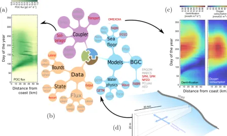
column hydrodynamic model GOTM, however, is replaced by the 3-D model GETM; a local wave component and data components for open boundaries and restart have been added. Figure 6 shows exchange fluxes between the water column and the sediment for 1 year of simulation. The simulation of turbidity, as a result of pelagic SPM transport and resuspen-sion by currents and wave stress, provides the light climate for the pelagic ecosystem. The flux of particulate organic car-bon (POC) into the sediment reflects bloom events in summer during calm weather conditions. Macrobenthic activity in the sea floor brings fresh organic matter into the deeper sub-oxic layers of the sediment, where denitrification removes nitro-gen from the pool of dissolved nutrients. The coupled simu-lation reveals decoupled signals of benthic respiration, den-itrification and nutrient reflux into the water column, which is not resolved in monolithically coded regional ecosystem models of the North Sea (Lorkowski et al., 2012; Daewel and Schrum, 2013).
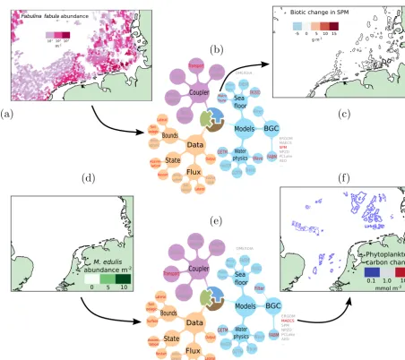
4.3 Southern North Sea bivalve ecosystem applications A southern North Sea (SNS) domain was used in two studies concerning the effects of bivalves on the pelagic ecosystem. Slavik et al. (2018) investigated how the accumulation of epi-fauna on wind turbine structures (Fig. 7d) impacts pelagic primary production and ecosystem functioning in the SNS on larger spatial scales. This study is the first of its kind that ex-trapolates the ecosystem impacts of anthropogenic offshore wind farm structures from a local to a regional sea scale. The authors use a MOSSCO coupled system consisting of the
hy-drodynamic model GETM, the ecosystem model MAECS as described by Kerimoglu et al. (2017), the transport connec-tor, the filter feeder component, and several input and out-put components (Fig. 7e). They assess the impact of anthro-pogenically enhanced filtration from blue mussel (Mytilus
edulis) settlement on offshore wind farms that are planned
to meet the 40-fold increase in offshore wind electricity in the European Union by 2030. They find a small but non-negligible large-scale effect in both phytoplankton stock and primary production, which possibly contributes to better wa-ter clarity (Fig. 7f).
Figure 6.A 2-D idealised cross-shore transect off the German coastline is used to investigate the feedback loop among estuarine circulation,
sediment transport, and nutrient cycling across the benthic–pelagic interface.(a, c)Hovmöller diagrams showing the soil–pelagic fluxes of
particulate organic carbon (POC) and the soil BGC denitrification and oxygen consumption rates for the 60 km long transect.(b)Coupling
diagram including components for hydrodynamics, erosion–sedimentation, waves, pelagic ecology, suspended particles, and soil ecology. This example uses both ESMF modularity (the components) and FABM modularity (the different ecological–biogeochemical models within
the pelagic and sediment environmental components).(d)Spatial set-up of the idealised 2-D cross-shore transect.
4.4 Exemplary workflow
For the SPM bivalve example above (Nasermoaddeli et al., 2018 and Fig. 7c), the coupled system contains 13 modular components: the hydrodynamic getm_component and simplewave_component, a pelagic fabm_component, the benthic erosion–sedimentation erosed_component and benthos_component, one output and four input components, the default link_connector, the nudge_connector, and the transport_connector. Each of these 13 compo-nents is involved in at least one pairwise coupling described in acouplingssection of the YAML coupling configura-tion (Fig. 3b). This coupled applicaconfigura-tion is to be deployed in sequential mode on the same set of computing resources for all 13 components.
The horizontal spatial representation and domain decom-position are provided by the grid that is created in the hy-drodynamic model and that is communicated to the wave, pelagic ecosystem, benthic, and input components; this is achieved by specifying the hydrodynamic model as a depen-dency of these components (dependenciesin Fig. 3b) Four instances of the netcdf_input_component (see
Sect. 3.2.2 and instances in Fig. 3b) are created to provide macrofauna forcing, lateral open ocean boundaries, rivers fluxes, and restart information from netCDF files. In the first of two initialisation phases, the output components and the hydrodynamic component are initialised first, as they have no dependencies. Dependent components then receive the spatial grid information from the hydrodynamic compo-nent. All components advertise what information they can provide (e.g. a certain quantity) and what information they need (e.g. grid information) in the coupled system.
Data Models Coupler Data BGC Bounds State Flux FABM ERGOM MAECS SPM NPZD PCLake AED ... OMEXDIA ... Transport Aggre-gation GETM HamSOM GOTM Tracer Wave Water physics Filter Makro fauna EROSED FABM Sea floor Micro flora Soil-pelagic Semantic mediation Grids Surface Lateral Assimi-lation Restart Atmo-spheric Soil-pelagic Lateral Soil-pelagic Source -sink Output
T. fabula abundance
100 101 102 103
Concentration (m−2)
101102103 m-1
Fabulina fabula abundance Biotic change in SPM
-5 0 5 10 15 g m-3
Data Models Coupler Data BGC Bounds State Flux FABM ERGOM MAECS SPM NPZD PCLake AED ... OMEXDIA ... Transport Aggre-gation GETM HamSOM GOTM Tracer Wave Water physics Filter Makro fauna EROSED FABM Sea floor Micro flora Soil-pelagic Semantic mediation Grids Atmo-spheric Lateral Assimi-lation Restart Atmo-spheric Soil-pelagic Lateral Soil-pelagic Source -sink Output
0.1 1.0 10 mmol m-3
Phytoplankton carbon change
5 10 0
M. edulis
abundance m-2
(a)
(b)
(c)
(d)
(e)
(f)
Figure 7.Building flexible applications with MOSSCO. Two bivalve-related scientific applications are showcased: Nasermoaddeli et al.
(2018) investigated the effect of bottom-dwellingFabulina fabula(a, showing parts of the southern North Sea) on suspended sediment
concentration(c)with a coupled application integrating hydrodynamics, three pelagic SPM classes in the ecosystem model, the mediation
of erodibility by benthic bivalves, and an explicit description of bed erosion and sedimentation(b); see Sect. 4.4 and Fig. 5. Slavik et al.
(2018) investigated the effect of epistructuralMytilus edulis(d)on phytoplankton concentration(f)with a coupled application integrating
hydrodynamics, the FABM–MAECS ecosystem model, and filtration by mussels(e).
input component that reads data from a file created in prior model runs (“restart”).
In the run phase, all pairwise couplings are called in the same order as during the initialisation phase. First, the con-nector (or coupler) is called to synchronise the two com-ponents’ data, then each of the coupled components in this pairwise coupling is executed for the minimum time inter-val to the next coupling time step of the involved compo-nents (see Fig. 2). With the boundary conditions read with the input component from files at each coupling interval, the SPM fields that reside in the ecosystem component are updated by way of connecting these components with the nudge_connector. Finally, at the end of a simulation,
all output components are run once more to ensure that the final state of the system is recorded; then, all components go through their finalisation phase and clean up reserved mem-ory.
5 Discussion and outlook
In merging existing frameworks that address distinct types of modularity and by developing a superstructure for making the multi-level coupling approach applicable in coastal re-search, the MOSSCO system largely meets the design goals
defi-ciencies of legacy models and the need for practical compro-mises became very apparent.
For legacy reasons, equitability is the harder to achieve de-sign goal. Both the distribution of computing resources and the spatial grid definition can in principle be determined by any one of the participating components; de facto, in marine or aquatic research, they are prescribed by the hydrodynamic models that have so far not been enabled to inherit a grid specification or a resource distribution from a coupler or cou-pled system. With the ongoing development and diversifica-tion of hydrodynamic models and no immediate benefit for the different physical models to outsource grid and resource allocation, this situation is not likely to change. MOSSCO compromises here with its flexible grid inheritance scheme and with the grid-provisioning component that delivers this information to the coupled system whenever a hydrodynamic component is not used.
Beyond grid and resource allocation, however, the equi-tability concept is successfully driving independent develop-ments of sub-modules. We found that experts in one partic-ular model, e.g. the erosion module, could rely on the func-tionality of the other parts of the system without having to be experts themselves in all of the constituent models in the cou-pled application. The limitations to this black-box approach became evident in the scientific application and evaluation of the coupled model system, which was only possible when collaboration with experts in these other model systems was sought. By taking away the inaccessibility barrier and by en-forcing a clear separation of tasks, the modular system stim-ulated a successful collaboration. Sustained granularity also helped in terms of alignment with ongoing development in external packages. These can be integrated fast into the cou-pled system, which does not rely on specific versions of the externally provided software unless structural changes occur. Long-term supported interfaces on the external model side facilitate MOSSCO being up to date with, for example, the fast-evolving GETM and FABM code bases.
When legacy codes were equipped with a framework– agnostic interface, we encountered four major difficulties.
1. For organising the data flow between the components, MOSSCO uses standard names and units compatible with the infrastructure and library of standard names and units provided in the pelagic component for the FABM framework (mostly modelled on CF). Other components, such as the BMIs of wrapped legacy mod-els, do not provide such a standard name in their own implementation and, in particular, often do not adhere to a naming standard. We found ambiguity arising, e.g. with temperature to be represented as temperaturevs.sea_water_temperaturevs. temperature_in_water. While this can be re-solved based on CF for temperature, most ecological and biogeochemical quantities currently lack a consis-tent naming scheme. The forthcoming GSN ontology
(building on CSDMS names; Peckham, 2014) could ad-equately address this coupling challenge.
2. Deep subroutine hierarchies of existing models made it difficult to isolate desired functionality from the struc-tural external overhead. In one example, in which a single functional module was taken out of the context of an existing third-party coupled system, the module depended on many routines dispersed throughout that third-party system repository.
3. Components based on stand-alone models are devel-oped and tested with their own I/O infrastructure and typically supply a BMI implementation only for part of their state and input data fields. A new coupled appli-cation or data provisioning and/or requesting within a coupled system can therefore easily require a change in a model BMI. The implementation potential input and output for all quantities, including replacement of the entire model-specific I/O in the BMI, is therefore desir-able for new developments and re-factoring.
4. Mass and energy need to be conserved across the cou-pled components. Mediators communicate conserva-tively regridded mass and energy fluxes into pairs of coupled components. These fluxes then need to be ap-propriately integrated by the coupled components, even when their internal time discretisation differs and for asynchronous scheduling that can incur different cou-pling time steps. The conservative integration of ex-changed mass and energy fluxes cannot automatically be ensured by the coupling system, and the user has to carefully consider time steps in the preparation of the coupling set-up.
Efforts to make legacy models coupleable, either for MOSSCO or similar frameworks, however, can have addi-tional benefits besides the immediate applicability in an in-tegrated context. Coupleability strictly demands the commu-nication of sufficient metadata, which stimulates the qual-ity and quantqual-ity of documentation and the scientific and technical reproducibility of legacy models. Indeed, trans-parency has been greatly increased by wrapping legacy mod-els in the MOSSO context. All participating components per-formed the introspection and leveraging of a collection of metadata at the assembly time of the coupled application and during output. Transparency is expected to be contin-uously increased by new coupling demands and more gen-erous metadata provisioning from wrapped science models. MOSSCO is moving towards adopting the Common Infor-mation Model (CIM) that is also required by Climate Model Intercomparison Project (CMIP) participating coupled mod-els (Eyring et al., 2016).
has not yet been tested; in the categorisation by de Laat (2007) internal governance with simple structure is sufficient at this size. Formally, external contributions can be included in MOSSCO by way of contributor licence agreements. The openness concept has been useful in instigating discussions about the need for explicit (and preferably open) licencing of related scientific software and data as demanded in current open science strategies (e.g. Scheliga et al., 2016).
Scalability in MOSSCO applications depends on the scala-bility of the coupled model components and on the potential overhead of the coupling infrastructure. Strong scaling ex-periments were performed with a coupled application using GETM, FABM with MAECS (≈20 additional transported 3-D tracers), and FABM with OMEXDIA_P, including bidi-rectional benthic–pelagic coupling, on Jureca (Krause and Thörnig, 2016). They show linear (perfect) scaling from 100 to 1000 cores and a small levelling-off (to 85% of per-fect scaling) at 3000 cores. We have not observed a loss of computing time due to the infrastructure and superstructure overhead of ESMF, which remained below 0.1 % in the run phase of the scaling experiment. A typical operational com-putation speed achieved, e.g. in the bivalve wind farm ap-plication (Sect. 4.3; 175 000 grid cells), on 192 processors is 2000 computed hours per elapsed wall clock hour: such a performance allows for decadal to multi-decadal simula-tions. One of the identified bottlenecks (that varies strongly with the HPC system used) is data transfer from memory to disc: this will be addressed in the future by the use of par-allel NetCDF and/or leveraging the XML I/O server (XIOS; Meursedoif, 2013).
Multi-component systems may also suffer from low ac-ceptance by the research community. They are much harder to implement and maintain by individual groups, in the con-text of which researchers solve coastal ocean problems of a large range of complexity, from purely hydrodynamic plications via coupled hydrodynamic–sediment dynamic ap-plications to fully coupled systems. Many academic prob-lems focus on specific mechanisms and thus do not require the complete and fully coupled modular system such that the application of the full system might mean a large structural overhead and additional workload. There is, however, the ne-cessity of following a holistic approach when tackling grand research questions in environmental science, such as those related to system responses to anthropogenic intervention. Yet, it is not clear whether the bottom-up approach of many interacting modular components leads to an emergent sys-tem behaviour that is desirable and exhibits new insights or whether the system gets tangled up in coupling complexity.
As evident from the test cases (Sect. 4), MOSSCO also encourages coupled applications that are far from a complete system-level description. With few coupled components, the technical threshold to getting an application running on an arbitrary system is relatively low. The user can quickly reach initial success. MOSSCO provides a full documentation, step by step recipes, and a public bug tracker; it adopts abundant
error reporting from ESMF and a fail fast design that stops a coupled application as soon as a technical error is detected (Shore, 2004). Usability is especially high due to an available master script that compiles, deploys, and schedules a coupled application. To address a wide range of users, the system is designed to run on a single processor or on a user’s laptop equally well as on a high-performance computer using sev-eral thousand computing nodes.
An obvious advantage of modular coupling is the opportu-nity to bridge the gap between different scientific disciplines. It allows in principle for the combination of, for example, hy-drodynamic models from oceanography with sediment trans-port models from coastal engineering. Thus different experts can work on their individual models but benefit from all oth-ers’ progress. This seeming advantage, however, also poses a drawback for modular coupling approaches. An initial effort which is necessary for individual models to meet the require-ments of a modular modelling framework has to be invested. This will only happen if there is either urgent pressure to include specific model capabilities, which will be difficult to include otherwise, or if convincing examples of possible ben-efits can be presented. It cannot be expected that the coastal ocean modelling community will agree about one coupler or one way of interfacing modules, so it will still require con-siderable implementation work to transfer a module from one modular system to another. To solve this problem, coupling standards need to become more general, but in turn this might even increase the structural overhead involved in using these systems.
For certain applications it might be preferable for differ-ent reasons to hardwire sub-models and exercise strong con-trol over such a monolithic coupled system. But at the least, such sub-models should be made coupleable by following the minimal requirements set forth by the BMI specification. This ensures that the monolithic model system or parts of it can be reused or expanded in a more modular way. And by strictly separating the BMI from any framework-specific CMI specification, the effort spent on wrapping an existing model or on equipping a new model with a basic model interface is not tied to a particular coupling framework or even a particular coupling framework technology. A model that follows BMI principles will be more easily interfaced to other models no matter what coupler is used. Wrapped legacy models from MOSSCO can thus be useful in non-ESMF con-texts as well, and models with an existing BMI can be inte-grated into MOSSCO more easily in turn.
anthro-pogenic measures. This ecosystem-based approach to man-agement (e.g. Ruckelshaus et al., 2008) demands modelling systems which are capable of taking into account hydrody-namics, biogeochemistry, sedimentology, and their interac-tions to properly describe the environmental status. As fur-ther legal requirements can be expected for many coastal seas worldwide, numerical modelling systems applied for this task need to be flexible in terms of integrating additional (e.g. site-specific) processes. In this ongoing process, the ini-tial effort of creating a modular system may be the only way forward that can take into account all relevant processes in the long run.
Outlook
The suite of components provided or encapsulated so far meets the demands that were initially formulated by our users; they already allow for a wide range of novel cou-pled applications to investigate the coastal sea. To stimulate more collaboration, however, and to bring forward a gen-eral “ecosystem” of modular science components, sevgen-eral legacy models could interface to MOSSCO components in the near future by building on complementary work at other institutions. For example, the Regional Earth System Model (RegESM; Turuncoglu et al., 2013; Turuncoglu and Sannino, 2017) provides ESMF interfaces for MITgcm, ROMS, and WAM, amongst others. The convergence of the development of MOSSCO and RegESM is feasible in the near term. Also, the recently developed Icosahedral Non-Hydrostatic Atmo-spheric Model (ICON; Zängl et al., 2015) is currently being equipped with an ESMF component model interface.
Once ESMF interfaces have been developed for a legacy model, it is desirable that these developments move out of the coupler system and become integrated into the devel-opment of the legacy model itself. This has been success-fully achieved with the ESMF interface for the hydrodynamic model GETM, which is now distributed with the GETM code. Much of the utility layer developed in MOSSCO, or likewise in MAPL or in the ESMF extension of the WRF model, is expected to be propagated upstream into the frame-work ESMF itself.
The interoperability of current coupling standards will in-crease. While currently there are three flavours of ESMF (ba-sic ESMF as in MOSSCO, ESMF–MAPL as in the GEOS-5 system, and ESMF–NUOPC as in the RegESM), only a minor effort would be required to provide the basic ESMF and ESMF–MAPL implementations with a NUOPC cap and make them interoperable with the entire ESMF ecosystem. Even a coupling of ESMF-based systems to OASIS-MCT-based systems has been proposed, and investigation is ongo-ing on a couplongo-ing of MOSSCO to the formal BMI for CS-DMS.
6 Conclusions
We problematised both the primacy of hydrodynamic mod-els and the limited modularity in coupled coastal modelling that can stand in the way of developing and applying novel and diverse biogeochemical process descriptions. Such de-velopmental potential is likely needed to progress towards holistic regional coastal systems models. We presented the novel Modular System for Shelves and Coasts (MOSSCO) that is built on coupling concepts centred around equitabil-ity and flexibilequitabil-ity to resolve the issue of obstructed modu-larity. These concepts also bring about openness, usability, transparency, and scalability. MOSSCO as a current Fortran implementation of this concept includes the wrapped Frame-work for Aquatic Biogeochemical Models (FABM) and a usability layer for the Earth System Modeling Framework (ESMF).
The MOSSCO design principles emphasise basic cou-pleability and rich meta-information. Basic coucou-pleability re-quires that models communicate about flow control, comput-ing resources, and exchanged data and metadata. We demon-strated that the design principles of flexibility and equi-tability enable the building of complex coupled models that adequately represent the complexity found in environmen-tal modelling. In this first version, the MOSSCO software wrapped several existing legacy models with basic model in-terfaces (BMIs); we added ESMF-specific component model interfaces (CMIs) to these wrappers and other models and frameworks to build a suite of ESMF components that when coupled represent a small part of a holistic coastal system. These components deal with hydrodynamics, waves, pelagic and sediment ecology and biogeochemistry, river loads, ero-sion, resuspenero-sion, biotic sediment modification, and filter feeding.
In selected applications, each with a different research question, the applicability of the coupled system was suc-cessfully tested. MOSSCO facilitates the development of new coupled applications for studying coastal processes that extend from the atmosphere through the water column into the seabed and that range from laboratory studies to 3-D sim-ulation studies of a regional sea. This system meets an infras-tructural need that is defined by experimenters and process modellers who develop biogeochemical, physical, sedimen-tological, or ecological models on the lab scale first and who would like to seamlessly embed these models into the com-plex coupled three-dimensional coastal system. This upscal-ing procedure may ultimately also support the global Earth system community.
(CC-BY-SA), a copyleft open document licence that allows the use, distribution, and modification of the documentation under the same terms.
Development code and documentation are currently primarily hosted on Sourceforge (https://sf.net/p/mossco/code) and mir-rored on Github (https://github.com/platipodium/mossco-code). The release version 1.0.1 is permanently archived on
Zen-odo and accessible under the digital object identifier
https://doi.org/10.5281/zenodo.438922.
Appendix A: Acronyms and model abbreviations used in the text
bash GNU Bourne Again SHell BFM Biogeochemical Flux Model
(ecosystem model) BGC Biogeochemistry
BMI Basic model interface (coupling concept) CC-BY-SA Creative Commons Attribution
Share-Alike licence
CF NetCDF Climate and Forecast convention CIM Common Information Model
(metadata standard) CMI Component model interface
(coupling concept)
CMIP Climate Model Intercomparison Project COAWST Coupled Ocean–Atmosphere–Wave–
Sediment Transport
CSDMS Community Surface Dynamics Modeling System
DKRZ Deutsches Klimarechenzentrum (HPC centre) ESM Earth system model
ESMF Earth System Modeling Framework FABM Framework for Aquatic
Biogeochemical Models FMS Flexible Modeling System
(coupling technology)
FONA Forschung für Nachhaltigkeit (funding scheme) FVCOM Finite-Volume Coastal Ocean Model
GCC GNU Compiler Collection
GETM General Estuarine Transport Model (3-D coastal ocean model)
GEOS-5 Goddard Earth Observing System version 5
GNU GNU is Not Unix
GOTM General Ocean Turbulence Model (1-D water column model) GPL General Public License
GSN Geoscience Standard Names Ontology HLRN Norddeutscher Verbund für
Hoch-und Höchstleistungsrechnen HPC High-performance computing ICON Icosahedral Non-Hydrostatic Model I/O Input and output
JSC Jülich Supercomputing Centre
MAPL Modeling Analysis and Prediction Layer MAECS Model for Adaptive Ecosystems
in Coastal Seas
MCT Model Coupling Toolkit
MESSy Modular Earth Submodel System MITgcm Massachusetts Institute of Technology
Global Circulation Model MOM Modular Ocean Model
MOSSCO Modular System for Shelves and Coasts MPI Message-passing interface
MSPD European Union Marine Strategic Planning Directive
NEMO Nucleus for European Modelling of the Ocean
NetCDF Network Common Data Form NPZD Nutrient, phytoplankton, zooplankton,
detritus (ecosystem model) NUOPC National Unified Operational
Prediction Capability
OASIS Ocean Atmosphere Sea Ice Soil coupler OMEXDIA Ocean Margin Exchange Experiment
early diagenetic model
OMEXDIA_P OMEXDIA with added phosphorous OMUSE Oceanographic Multipurpose Software
Environment
PARSE Prepare, adapt, register, schedule, execute methodology
PISCES Pelagic Interactions Scheme for Carbon and Ecosystem Studies POM Particulate organic matter POC Particulate organic carbon RegESM Regional Earth System Model ROMS Regional Ocean Modeling System SCRIP Spherical Coordinate Remapping and
Interpolation Package
SNS Southern North Sea
SPM Suspended particulate matter SWAN Simulating Waves Nearshore WAM Wave atmospheric model
WFD European Union Water Framework Directive
![(Acetato κO){bis[(2,4 dimethyl 1H pyrazol 1 yl)methyl][(pyridin 2 yl)methyl]amine}cobalt(II) hexafluoridophosphate](data:image/gif;base64,R0lGODlhAQABAIAAAP///wAAACH5BAEAAAAALAAAAAABAAEAAAICRAEAOw==)