www.geosci-model-dev.net/7/1873/2014/ doi:10.5194/gmd-7-1873-2014
© Author(s) 2014. CC Attribution 3.0 License.
SimSphere model sensitivity analysis towards establishing its use for
deriving key parameters characterising land surface interactions
G. P. Petropoulos1, H. M. Griffiths1, T. N. Carlson2, P. Ioannou-Katidis1, and T. Holt1
1Department of Geography and Earth Sciences, Aberystwyth University, Aberystwyth, SY23 2DB, UK 2Department of Meteorology, Pennsylvania State University, University Park, PA 16802, USA
Correspondence to: G. P. Petropoulos ([email protected])
Received: 2 October 2013 – Published in Geosci. Model Dev. Discuss.: 7 January 2014 Revised: 25 June 2014 – Accepted: 25 June 2014 – Published: 2 September 2014
Abstract. Being able to accurately estimate parameters
char-acterising land surface interactions is currently a key scien-tific priority due to their central role in the Earth’s global energy and water cycle. To this end, some approaches have been based on utilising the synergies between land surface models and Earth observation (EO) data to retrieve relevant parameters. One such model is SimSphere, the use of which is currently expanding, either as a stand-alone application or synergistically with EO data. The present study aimed at exploring the effect of changing the atmospheric sounding profile on the sensitivity of key variables predicted by this model assuming different probability distribution functions (PDFs) for its inputs/outputs. To satisfy this objective and to ensure consistency and comparability to analogous studies conducted previously on the model, a sophisticated, cutting-edge sensitivity analysis (SA) method adopting Bayesian theory was implemented on SimSphere. Our results did not show dramatic changes in the nature or ranking of influen-tial model inputs in comparison to previous studies. Model outputs examined using SA were sensitive to a small number of the inputs; a significant amount of first-order interactions between the inputs was also found, suggesting strong model coherence. Results showed that the assumption of different PDFs for the model inputs/outputs did not have an important bearing on mapping the most responsive model inputs and interactions, but only the absolute SA measures. This study extends our understanding of SimSphere’s structure and fur-ther establishes its coherence and correspondence to that of a natural system’s behaviour. Consequently, the present work represents a significant step forward in the global efforts on SimSphere verification, especially those focusing on the de-velopment of global operational products from the model synergy with EO data.
1 Introduction
Understanding the natural processes of the Earth as well as how the different components (i.e. lithosphere, hydrosphere, the biosphere and atmosphere) of the Earth’s systems inter-play, especially in the context of global climate change, has been recognised by the global scientific community as a very urgent and important research direction requiring further in-vestigation (Battrick et al., 2006). This requirement is also of crucial importance for addressing directives such as the EU Water Framework Directive. To this end, being able to accu-rately obtain spatio-temporal estimates of parameters such as the latent (LE) and sensible (H) heat fluxes as well as of soil moisture is of great importance. This is due to their important role in many physical processes characterising land surface interactions of the Earth system as well as their practical use in a wide range of multidisciplinary studies and applications (Kustas and Anderson, 2009; Seneviratne et al., 2010).
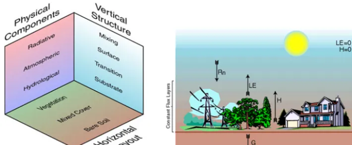
Figure 1. Left: the different layers of the SVAT model in the vertical domain; right: a schematic representation of the surface energy balance
components computation in the SVAT model (after SimSphere user’s manual available at http://www.aber.ac.uk/en/iges/research-groups/ earth-observation-laboratory/simsphere/workbook/preface/).
One such group of approaches, the so-called “triangle” method (Carlson, 2007), is used to predict regional esti-mates of LE, H fluxes and soil moisture content (SMC). SimSphere is a soil–vegetation–atmosphere–transfer (SVAT) model, originally developed by Carlson and Boland (1978) and considerably modified to its current state by Gillies et al. (1997) and Petropoulos et al. (2013a). SVAT models are essentially mathematical representations of one-dimensional “views” of the physical mechanisms controlling energy and mass transfers in the soil–vegetation–atmosphere continuum, providing deterministic estimates of the time course of vari-ous variables characterising land surface interactions at time steps appropriate to the dynamics of atmospheric processes (Olioso et al., 1999). An overview of SimSphere use was re-cently provided by Petropoulos et al. (2009a). The different facets of the SVAT model’s overall structure – namely the physical, the vertical and the horizontal – are illustrated in Fig. 1 (left). An extensive mathematical description of the model can be found in Carlson and Boland (1978), Carlson et al. (1981) and Gillies and Carlson (1995). The Sim-Sphere model is maintained and is distributed freely globally (both the executable version and model code) from Aberys-twyth University, United Kingdom (http://www.aber.ac.uk/ simsphere).
As regards the triangle method in particular, it has its foun-dations in the physical properties encapsulated in a satellite-derived scatterplot of surface temperature (Ts) and vege-tation index (VI), linked with SimSphere. Petropoulos et al. (2009b) have underlined the potential of this group of approaches for operational implementation in deriving es-timates of LE/H fluxes and/or SMC. A recent description of the triangle workings can be found in Petropoulos and Carlson (2011). At present, variants of this method are ex-plored – or even some already implemented in practice – for deriving, in some cases operationally and on a global scale, estimates of LE andHfluxes and/or SMC (Chauhan et al., 2003; Piles et al., 2011; ESA STSE, 2012). In addition,
SimSphere use is continually expanding worldwide both as an educational and as a research tool – used either as a stand-alone application or synergistically with EO data – to con-duct studies aiming to improve understanding of land surface processes and their interactions. Considering the research and practical work with respect to SimSphere use, it is ev-idently of primary importance to execute a variety of valida-tory tests to evaluate its adequacy and coherence in terms of its ability to accurately and realistically represent Earth’s surface processes.
Performing a sensitivity analysis (SA) provides an impor-tant and necessary validatory component of any computer simulation model or modelling approach before it is used in performing any kind of analysis. SA allows determining the effect of changing the value of one or more input vari-ables of a model and observing the consequence that this has on given outputs simulated by the model. Its implementa-tion on a model allows understanding the model’s behaviour, coherence and correspondence to what it has been built to simulate (Saltelli et al., 1999, 2000; Nossent et al., 2011). As such, SA provides a valuable method to identify signifi-cant model inputs as well as their interactions and rank them (Chen et al., 2012), offering guidance to the design of exper-imental programs as well as to more efficient model coding or calibration. Indeed, by means of a SA unrelated parts of the model may be dropped or a simpler model can be built or extracted. The latter can reduce, in some cases significantly, the required computing power while maintaining the mod-els’ correspondence to a natural system’s behaviour in the real world (Holvoet et al., 2005).
model’s inputs. The sensitivity of the input parameters is examined based on the use of samples derived directly from the model, which are distributed across the parameter domain of interest. These methods, despite their high computational demands, have become popular in environmental modelling due to their ability to incorporate parameter interactions and their relatively straightforward interpretation (Nossent et al., 2011). They also account for the influence of the input pa-rameters over their whole range of variation, which in turn enables obtaining SA results independent of any “modelers’ prejudice”, or site-specific bias (Song et al., 2012).
Petropoulos et al. (2009a) in a recent review of SimSphere exploitation underlined the importance of carrying out SA experiments on the model, as part of its overall verification. In response, Petropoulos et al. (2009c, 2010, 2013b, c, d) performed advanced GSA on SimSphere based on a Gaus-sian process (GP) emulator. As previous SA studies on Sim-Sphere had been scarce, their results provided for the first time an insight into the model architecture, allowing the map-ping of the sensitivity between the model inputs and key model outputs. Although all the model input parameters were varied across their full range of variation by those studies, a particular atmospheric sounding setting had been used in these GSA experiments by the authors. In addition, the effect of different probability distribution functions (PDFs) for the model inputs/outputs to the obtained had not been adequately explored.
In this context, the aim of the present study was to perform a GSA on SimSphere using an atmospheric sounding derived from a different region and evaluate the effect of atmospheric sounding on the SA results obtained on SimSphere assuming different PDFs for the model inputs/outputs. This will allow us to extend our understanding of this model structure and further establishing its coherence.
2 The Bayesian sensitivity analysis method
To satisfy the objectives of this study and to ensure con-sistency and comparability of our work to previous stud-ies on SimSphere, SA is conducted here by employing a sophisticated, cutting-edge GSA method adopting Bayesian Analysis of Computer Code Outputs (BACCO; Kennedy and O’Hagan, 2001). It is implemented using the Gaus-sian Emulation Machine (GEM)-SA software, the develop-ment of which was funded by the National Environmen-tal Research Council, United Kingdom. The theory behind the BACCO GEM-SA technique can be found by Oakley and O’Hagan (2004); detailed descriptions of the mathemat-ical principles governing the GP emulation are available in Kennedy and O’Hagan (2001), Kennedy (2004) and Oakley and O’Hagan (2004). The use of the GPs to model unknown functions in Bayesian statistics dates back to Kimeldorlf and Wahba (1970) and O’Hagan (1978).
Briefly, BACCO GEM-SA implementation consists of two phases: first, a statistically based representation (i.e. an emu-lator) of the model is built from training data obtained from simulations derived from the actual model, which have been designed to cover the multidimensional input space using a space-filling algorithm. Second, the emulator itself is used to compute a number of statistical parameters to characterise the sensitivity of the targeted model output in respect to its inputs.
BACCO SA implementation starts from a prior belief about the code (i.e. that it has no numerical error), and then – based on a GP model, Bayes’ theorem and a set of the model code runs – this assumption is refined to yield the posterior distribution of the output, which is the emulator. In building the emulator, the most important prior assumption is that the output emulator is a reasonably smooth function of its in-puts. On this basis, the emulator is used to calculate a mean function, which attempts to pass through the observed runs at the same time it quantifies the remaining uncertainty due to the emulator being an approximation to the true code. Within BACCO, various statistical measures are generated automat-ically when the emulator is built in order to check the accu-racy of both types of output.
In simple mathematical terms, the basic SA output from GEM-SA includes a direct decomposition of the model out-put variance into factorial terms, called “importance mea-sures” (e.g. Ratto et al., 2001):
V (Y )=
s
X
i=1 Di+
X
iCj
Dij+. . .+D1...s (1)
Di=V (E(Y|Xi)), (2)
Dij=V (E(Y
Xi, Xj))−V (E(Y
Xi))
−V (E(YXj)), (3)
wheresdenotes the number of inputs (so-called “factors”),
−V (Y ) is the total variance of the output variableY,Di is
the importance measure for inputXi,Dij is the importance
measure for the interaction between inputsXiandXj,D1...s
denote similar formulae for the higher-order terms.E(Y|Xi)
is the conditional expectation ofY given a value ofXi and
the variance ofE(Y|Xi)is taken over all inputs factors which
are fixed in the conditional expectations.
In addition, in the BACCO method, sensitivity indices are computed by dividing the importance measures from Eq. (1) by the total output variance as follows:
Si=
Di
V (Y ) , Sij = Dij
V (Y ). (4)
These ratiosSi fori=1, . . . , s are called main effects or
first-order sensitivity indices, because eachSi delivers a
di-rect measure of the share of the output variance explained by X. The main effect or first-order sensitivity index Si is the
(within its uncertainty range). Thus, this is a measure that quantifies the relative importance of an individual input vari-able Xi, in driving the total output uncertainty, indicating
where to direct future efforts to reduce that uncertainty. Us-ing similar formulae, higher-order sensitivity indices (joint effect indices) are also computed in GEM-SA to compute the sensitivity of the model output to input parameter inter-actions. However, in practice, because the estimation ofSior
Sij, or higher order, can be computationally very expensive,
the SA is rarely carried out further after the computation of first-order interaction indices (i.e. the second term of Eq. 5 below). This is also the case with GEM-SA.
Thus, from the definitions of the above indices, and assum-ing non-correlated inputs, a complete series development of the output variance can be achieved:
X
i
Si+
X
iCj
Sij+
X
iCjCm
Sij m+. . .+S12...k=1, (5)
where higher-order indices are defined in a similar way to Eq. (7). This decomposition of variance into main effects and interactions is commonly known as analysis of variance– high-dimensional model representation (HDMR).
The percentage variance contribution of each input’s main effect is also reported in BACCO, providing a simple means of ranking the inputs in terms of their importance. The per-centage variance component associated with each input mea-sures the amount its main effect contributes to the total output variance, based on the uncertainty distributions for all inputs. It should be noted that, in general, summing the main effect contributions will not total to 100 % because of the additional contributions from the interaction effects. However, the total can be used to determine the degree of interactions.
In addition to the above indices, another measure that is computed in GEM-SA is the total sensitivity index. This is used to provide a cheaper computational method of investi-gating the higher-order sensitivity effects as it collects all the interactions involvingXiin one single term. The total
sensi-tivity index of a given factorXi takes into account the main
effect and the effect of all its interactions with other model inputs, and is defined as
STi=
Di+Di,∼i
V (Y ) , (6)
whereDi,∼i indicates all interactions between factorXi and
all the others (X∼i).
The total sensitivity index represents the expected amount of output variance that would remain unexplained (residual variance) if only Xi were left free to vary over its range,
the value of all other variables being known. The useful-ness of the STi is that it is possible to compute them
with-out necessarily evaluating the single indicesSi (and
higher-order ones), making the analysis computationally affordable. The total sensitivity indices are generally used to identify unessential variables (i.e. those that have no importance ei-ther singularly or in combination with oei-thers) while building
a model. The existence of large total effects relative to main effects implies the presence of interactions among model in-puts.
The BACCO method has already supplied useful insights in various disciplines and in various SA studies underly-ing the advantages of this approach (Kennedy and O’Hagan, 2001; Johnson et al., 2011; Kennedy et al., 2012; Parry et al., 2012). Petropoulos et al. (2009c) demonstrated for the first time the use of the BACCO method in performing a SA on SimSphere, providing an insight into the model struc-ture. Petropoulos et al. (2010) performed a comparative study of various emulators including BACCO GEM, investigating the effect of sampling method and size on the sensitivity of key target quantities simulated by SimSphere. Their results showed that the sampling size and method did affect the SA results in terms of absolute values, but had no bearing in iden-tifying the most sensitive model inputs and their interactions, for model outputs on which SA was performed.
3 Sensitivity analysis implementation
To ensure consistency and comparability with previous anal-ogous SA studies on SimSphere, the BACCO GEM-SA was implemented herein along the lines of previous similar GSA studies applied to that model (Petropoulos et al., 2009c, 2010, 2013b, c, d). The only difference was the use of a dif-ferent atmospheric sounding profile derived from a difdif-ferent location and season. Thus, the sensitivity of the following SimSphere outputs was evaluated:
– Daily Average Net Radiation (Rndaily),
– Daily Average Latent Heat flux (LEdaily),
– Daily Average Sensible Heat flux (Hdaily),
– Daily Average Tair (Tairdaily),
– Daily Average Surface Moisture Availability (Modaily),
– Daily Average Evaporative Fraction (EFdaily),
– Daily Average Non-Evaporative Fraction (NEFdaily),
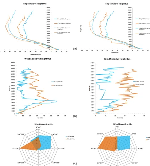
Figure 2. Atmospheric soundings used in the present study in comparison to the Petropoulos et al. (2009c) study for temperature (a, b), wind
direction (c, d) and wind speed (e, f).
ranges of values were defined from the entire possible theo-retical range which they could take in SimSphere parameter-isation (Table 1). The potential of co-variation between the parameters was assumed negligible, as in previous studies. In addition, the emulator performance was evaluated based on
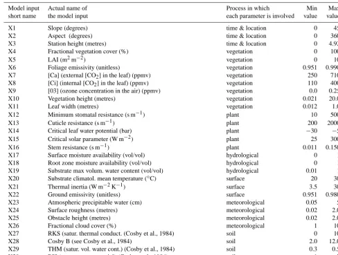
Table 1. Summary of the SimSphere inputs considered in the GSA implementation. Units of each of the model inputs, where appropriate,
are provided in brackets.
Model input Actual name of Process in which Min Max
short name the model input each parameter is involved value value
X1 Slope (degrees) time & location 0 45
X2 Aspect (degrees) time & location 0 360
X3 Station height (metres) time & location 0 4.92
X4 Fractional vegetation cover (%) vegetation 0 100
X5 LAI (m2m−2) vegetation 0 10
X6 Foliage emissivity (unitless) vegetation 0.951 0.990
X7 [Ca] (external [CO2] in the leaf) (ppmv) vegetation 250 710
X8 [Ci] (internal [CO2] in the leaf) (ppmv) vegetation 110 400
X9 [03] (ozone concentration in the air) (ppmv) vegetation 0.0 0.25
X10 Vegetation height (metres) vegetation 0.021 20.0
X11 Leaf width (metres) vegetation 0.012 1.0
X12 Minimum stomatal resistance (s m−1) plant 10 500
X13 Cuticle resistance (s m−1) plant 200 2000
X14 Critical leaf water potential (bar) plant −30 −5
X15 Critical solar parameter (W m−2) plant 25 300
X16 Stem resistance (s m−1) plant 0.011 0.150
X17 Surface moisture availability (vol/vol) hydrological 0 1
X18 Root zone moisture availability (vol/vol) hydrological 0 1
X19 Substrate max volum. water content (vol/vol) hydrological 0.01 1
X20 Substrate climatol. mean temperature (◦C) surface 20 30
X21 Thermal inertia (W m−2K−1) surface 3.5 30
X22 Ground emissivity (unitless) surface 0.951 0.980
X23 Atmospheric precipitable water (cm) meteorological 0.05 5
X24 Surface roughness (metres) meteorological 0.02 2.0
X25 Obstacle height (metres) meteorological 0.02 2.0
X26 Fractional cloud cover (%) meteorological 1 10
X27 RKS (satur. thermal conduct. (Cosby et al., 1984) soil 0 10
X28 Cosby B (see Cosby et al., 1984) soil 2.0 12.0
X29 THM (satur. vol. water cont.) (Cosby et al., 1984) soil 0.3 0.5
X30 PSI (satur. water potential) (Cosby et al., 1984) soil 1 7
4 Results
4.1 Emulator validation
The uncertainty of the SA due to the performance of the emulator was evaluated on the basis of a number of statis-tical measures computed internally by GEM-SA. Those in-cluded the validation root mean square error”, validation root mean squared relative error” and the “cross-validation root mean squared standardised error”. In addi-tion a unitless parameter called “roughness value”, also com-puted internally in GEM-SA, was used. This parameter pro-vides an estimate of the changes in model outputs in response to changes in the inputs to the model. Finally, the “sigma-squared” statistical parameter, also computed within GEM-SA, was also used to statistically appreciate the performance of the emulator build. Within BACCO GEM-SA, this ex-presses the variance of the emulator after standardising the
output, and effectively provides a measure of the quality of the fit of the emulator to the original model code.
forHdaily, and aspect, fractional vegetation cover, vegetation height and Mo for Traddaily). Noticeably, the results obtained herein in regards to the emulator accuracy were largely com-parable to previous GSA studies on SimSphere (Petropoulos et al., 2009c, 2013b, c, d), suggesting a good emulator build able to emulate the target quantities examined reasonably ac-curately.
4.2 SA results
Tables 4 and 5 summarise the relative sensitivity of the model outputs with respect to its inputs, for both the cases of normal and uniform PDF assumptions for the model inputs/outputs. Input parameters with a main effect>1 % and/or>1 % total effect are highlighted in bold. Figure 3 exemplifies the main effect and total effects for each model output of which the SA was examined. The following sections systematically de-scribe the main results obtained in terms of the SA for both cases of PDF assumption, focusing primarily on the analysis of the main and total SA indices computed.
4.2.1 Parameter sensitivity for Rndaily
Main effects and total effects from 0 to 50.1 % and 0 to 63.6 %, respectively, for normal PDFs (Table 4, Fig. 3) and from 0 to 48.1 % and 0 to 65.7 % (Table 5), respectively, in the case of uniform PDF assumption. Under normal PDF assumption, the inputs with the largest percentage variance contribution were aspect (50.1 %), slope (20.3 %) and Fr (7.2 %), and LAI (2.1 %) and Mo (3.6 %) were also relevant. As Table 4 shows, these parameters also contributed signif-icantly to the total effects, although vegetation height also contributed here (1.2 %). Clearly, changing the PDFs to uni-form did not significantly alter the nature or the ranking of the most important model inputs (Table 5, Fig. 3). Yet, it is noticeable that for this PDF assumption, surface roughness input became more important, contributing 1.1 % to the to-tal effects. In summary, the model input parameters with the highest total effects (i.e. those to which Rndailyis most sensi-tive) were aspect, slope, Fr, LAI, Mo, vegetation height and surface roughness. Only nine significant (>0.1 %) first-order interactions were found for this parameter assuming a normal PDF and assuming a uniform PDF for the model inputs. As-suming a uniform PDF, the most significant first-order inter-actions were between slope and aspect (13.4 %) and between Fr and LAI (0.6 %). For normal PDFs the interaction between slope and aspect was by far the most important (10.20 %). In-teractions between aspect and Fr (0.4 %), Fr and LAI (0.3 %) and aspect and Mo (0.3 %) were also significant.
4.2.2 Parameter sensitivity forHdaily
Main effects and total effects were lower in this case and ranged from 0 to 15.2 % and from 0 to 31.1 %, respectively, for normal PDFs (Table 4) and from 0 to 16.6 % and 0 to 30.4 %, respectively, for uniform PDFs (Table 5). Under
normal PDFs, the inputs parameters with the largest percent-age variance contribution were Fr (15.2 %), Mo (11.7 %), as-pect (10.9 %) and vegetation height (10.4 %). Surface rough-ness (3.5 %) and slope (1.4 %) were also important. In terms of the total effects, aspect was the most important parameter (31.1 %) for the simulation ofHdailyby the model, followed by vegetation height (29.7 %), Mo (26.3 %) and Fr (25.5 %). A number of other parameters also showed significant total effects (Table 4). The nature and rank of significant input parameters to main effects was also not changed by chang-ing the PDFs to uniform (Table 5, Fig. 3). In terms of the total effects, however, vegetation height becomes the most important by a small margin (30.4 % compared to 30.1 % for aspect). Numerous important input parameters are seen to influence Hdaily therefore, with the most important be-ing aspect, Fr, vegetation height, Mo and surface rough-ness. A large number of first-order interactions with values higher than 0.1 % were observed forHdailyassuming a uni-form PDF (32 in total) and assuming a normal PDF (39 in total). Assuming a uniform PDF the most important inter-actions were between vegetation height and surface rough-ness (4.76 %), Fr and Mo (2.46 %), Fr and vegetation height (1.95 %), aspect and surface roughness (1.67 %) and aspect and Mo (1.40 %). The most significant interaction assum-ing a normal PDF was between vegetation height and sur-face roughness (4.31 %), but interactions between aspect and surface roughness (2.52 %), Mo (1.71 %), vegetation height (1.13 %) and O3 in the air (0.72 %) as well as interactions between Fr and Mo (2.26 %) and vegetation height (1.91 %) were also found. In terms of second-order or higher inter-actions, a higher level of significant interactions was found, with 16.8 and 21.9 % noted assuming normal and uniform PDFs, respectively.
4.2.3 Parameter sensitivity for LEdaily
Table 2. Emulator accuracy statistics for the SA tests conducted in our study (under both normal and uniform PDF assumptions for the model
inputs/outputs).
Fitted model parameters (based on standardised input/output) Rndaily Hdaily LEdaily Traddaily Modaily Tairdaily EFdaily NEFdaily
Sigma-squared: 0.413 1.619 1.057 0.875 1.240 1.630 1.483 1.483
Emulator accuracy:
Cross-validation root mean squared error (W m−2): 25.060 34.776 28.798 2.771 31.012 0.491 0.082 0.082 Cross-validation root mean squared relative error (%): 6.349 41.633 23.485 7.913 13.814 3.030 20.033 25.292 Cross-validation root mean squared standardised error: 1.111 1.790 1.484 1.117 1.474 1.505 1.717 1.717
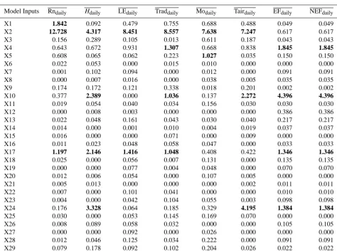
Table 3. Summarised statistics concerning the emulator accuracy evaluation for the different SimSphere model outputs examined in our
study. Bold font highlights the roughness values of the model inputs with values greater than 1.0. Rows X1 to X30 show roughness values for the different model outputs examined (for normal and uniform PDFs).
Model Inputs Rndaily Hdaily LEdaily Traddaily Modaily Tairdaily EFdaily NEFdaily
X1 1.842 0.092 0.479 0.755 0.688 0.488 0.049 0.049
X2 12.728 4.317 8.451 8.557 7.638 7.247 0.617 0.617
X3 0.156 0.289 0.105 0.013 0.611 0.187 0.043 0.043
X4 0.643 0.672 0.931 1.307 0.668 0.838 1.845 1.845
X5 0.608 0.065 0.062 0.223 1.027 0.035 0.150 0.150
X6 0.022 0.053 0.000 0.015 0.010 0.000 0.000 0.000
X7 0.001 0.102 0.094 0.000 0.012 0.000 0.091 0.091
X8 0.000 0.007 0.016 0.000 0.038 0.005 0.035 0.035
X9 0.174 0.172 0.121 0.338 0.018 0.201 0.002 0.002
X10 0.377 2.389 0.000 1.036 0.137 2.272 4.396 4.396
X11 0.019 0.054 0.040 0.034 0.156 0.030 0.030 0.030
X12 0.000 0.008 0.003 0.000 0.000 0.000 0.386 0.386
X13 0.022 0.048 0.161 0.043 0.030 0.040 0.217 0.217
X14 0.014 0.000 0.001 0.010 0.004 0.019 0.037 0.037
X15 0.016 0.000 0.000 0.071 0.000 0.009 0.000 0.000
X16 0.011 0.023 0.048 0.058 0.047 0.000 0.033 0.033
X17 1.197 2.146 1.416 1.048 0.408 0.422 1.346 1.346
X18 0.025 0.000 0.056 0.007 0.131 0.000 0.135 0.135
X19 0.000 0.000 0.077 0.004 0.048 0.000 0.070 0.070
X20 0.012 0.006 0.054 0.000 0.107 0.005 0.000 0.000
X21 0.005 0.013 0.000 0.000 0.000 0.002 0.011 0.011
X22 0.007 0.000 0.101 0.041 0.000 0.000 0.010 0.010
X23 0.004 0.000 0.042 0.104 0.055 0.003 0.098 0.098
X24 0.176 3.328 0.064 0.185 0.329 4.195 1.384 1.384
X25 0.030 0.000 0.053 0.145 0.169 0.070 0.000 0.000
X26 0.008 0.089 0.058 0.032 0.000 0.000 0.105 0.105
X27 0.000 0.000 0.092 0.000 0.026 0.000 0.000 0.000
X28 0.012 0.046 0.125 0.034 0.222 0.000 0.091 0.091
X29 0.079 0.178 0.092 0.102 0.204 0.026 0.022 0.022
X30 0.079 0.006 1.710 0.083 0.054 0.174 0.003 0.003
of LEdailywere aspect, Mo, Fr and slope. Assuming uniform PDFs for the model inputs, two first-order interactions domi-nate for this parameter – those between slope and aspect once more (6.8 %) and those between Fr and Mo (6.8 %). Inter-actions between aspect and Mo (1.0 %) and Fr (4.6 %), re-spectively, are also important. When normal PDFs for model inputs/outputs were assumed, 24 first-order interactions with values higher than 0.1 % were observed, and, once again, the interaction between slope and aspect (6.1 %) were the most important. However, important interactions between Fr and
Mo (4.6 %), aspect and Mo (1.2 %) and between aspect and Fr (0.8 %) were also observed.
4.2.4 Parameter sensitivity for Traddaily
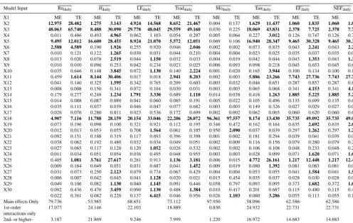
Table 4. Summarised results from the implementation of the BACCO GEM-SA method on the different outputs simulated by SimSphere
using the normal PDFs. Computed main (ME) and total effect (TE) indices by the GEM tool (expressed as %) for each of the model parameters are shown, whereas the last three lines summarise the percentages of the explained total output variance of the main effects alone and after including the interaction effects. Input parameters with a variance decomposition of greater than 1 % are highlighted in bold font.
Model Input Rndaily Hdaily LEdaily Traddaily Modaily Tairdaily EFdaily NEFdaily
ME TE ME TE ME TE ME TE ME TE ME TE ME TE ME TE
X1 20.294 31.964 1.388 3.078 7.969 16.245 12.676 24.032 17.129 29.450 1.846 10.150 0.991 1.613 0.991 1.613 X2 50.095 63.626 10.944 31.147 36.024 51.870 34.857 52.048 28.462 50.207 21.877 43.797 4.283 8.883 4.283 8.882 X3 0.016 0.353 0.469 4.245 0.066 0.825 0.031 0.150 1.278 4.853 0.411 2.482 0.130 0.610 0.130 0.610 X4 7.161 8.916 15.239 25.509 8.132 16.975 5.586 10.606 0.704 6.702 16.655 25.647 10.362 26.932 10.362 26.932 X5 2.060 3.357 0.135 1.710 0.184 0.709 0.049 1.462 12.028 20.080 0.071 0.672 0.060 1.824 0.060 1.824 X6 0.014 0.094 0.142 1.136 0.027 0.028 0.048 0.177 0.030 0.151 0.020 0.022 0.032 0.034 0.032 0.034 X7 0.010 0.015 0.090 2.166 0.049 0.855 0.028 0.029 0.054 0.198 0.037 0.039 0.065 1.086 0.065 1.086 X8 0.008 0.008 0.120 0.262 0.031 0.181 0.020 0.021 0.065 0.474 0.102 0.200 0.060 0.544 0.060 0.544 X9 0.029 0.465 0.093 3.309 0.098 0.898 0.149 1.703 0.032 0.222 0.067 2.669 0.093 0.120 0.093 0.120 X10 0.427 1.234 10.357 29.664 0.015 0.016 3.293 7.415 0.803 2.066 7.832 22.447 8.155 24.214 8.155 24.214 X11 0.021 0.095 0.275 1.401 0.350 0.677 0.127 0.432 0.177 2.093 0.044 0.500 0.308 0.759 0.308 0.759 X12 0.006 0.007 0.137 0.306 0.065 0.091 0.026 0.027 0.033 0.034 0.058 0.060 0.442 3.400 0.442 3.400 X13 0.134 0.203 0.158 1.041 1.546 2.699 0.609 0.922 0.151 0.490 0.247 0.929 1.652 4.295 1.653 4.295 X14 0.013 0.066 0.088 0.090 0.037 0.052 0.074 0.155 0.131 0.174 0.097 0.395 0.155 0.599 0.155 0.599 X15 0.024 0.077 0.037 0.039 0.041 0.042 0.070 0.506 0.030 0.031 0.122 0.260 0.025 0.026 0.025 0.026 X16 0.021 0.057 0.242 0.717 0.021 0.422 0.168 0.563 0.042 0.648 0.055 0.057 0.042 0.477 0.042 0.477 X17 3.554 5.219 11.669 26.284 17.567 27.166 16.911 21.465 3.563 7.129 7.010 11.169 38.200 49.518 38.199 49.518 X18 0.071 0.160 0.099 0.101 0.251 0.707 0.095 0.159 0.054 1.229 0.143 0.145 0.835 2.507 0.835 2.507 X19 0.010 0.010 0.054 0.056 0.643 1.300 0.056 0.090 0.284 0.735 0.033 0.035 0.286 1.055 0.286 1.056 X20 0.083 0.125 0.190 0.308 0.098 0.538 0.346 0.347 0.749 1.608 0.167 0.256 0.036 0.038 0.036 0.038 X21 0.032 0.050 0.228 0.487 0.029 0.030 0.043 0.044 0.035 0.037 0.105 0.137 0.072 0.234 0.072 0.234 X22 0.016 0.043 0.119 0.121 0.130 0.841 0.043 0.449 0.055 0.057 0.094 0.096 0.045 0.194 0.045 0.194 X23 0.009 0.025 0.052 0.054 0.032 0.378 0.042 0.718 0.124 0.653 0.025 0.081 0.066 1.239 0.066 1.239 X24 0.285 0.745 3.509 24.425 0.222 0.707 0.853 2.332 1.391 4.019 6.465 23.644 1.318 9.913 1.318 9.913 X25 0.010 0.129 0.049 0.051 0.044 0.552 0.051 1.067 0.061 1.551 0.042 1.070 0.075 0.076 0.075 0.076 X26 0.030 0.059 0.264 2.020 0.079 0.625 0.087 0.368 0.051 0.052 0.047 0.049 0.050 1.240 0.050 1.240 X27 0.005 0.005 0.043 0.045 0.032 0.909 0.017 0.018 0.053 0.330 0.031 0.033 0.026 0.028 0.026 0.028 X28 0.035 0.075 0.072 1.019 0.044 0.882 0.049 0.321 0.374 2.540 0.082 0.084 0.224 1.261 0.224 1.261 X29 0.058 0.289 0.402 2.995 0.028 0.866 0.344 1.024 0.103 2.105 0.206 0.585 0.118 0.404 0.118 0.404 X30 0.036 0.276 0.074 0.199 0.285 5.121 0.096 0.781 0.042 0.661 0.071 2.333 0.052 0.099 0.052 0.099 Main effects only 84.568 56.735 74.138 76.844 68.091 64.061 68.258 68.258 1st-order
interactions only
13.486 26.454 19.706 17.916 24.610 24.309 22.129 22.129
2nd- or higher-order interactions
1.946 16.810 6.155 5.240 7.299 11.630 9.613 9.613
important model inputs were aspect (34.9 %), Mo (16.9 %) and slope (12.7 %), with Fr and vegetation height also im-portant. This is mirrored in the total effects, but here LAI, [O3] in the air, surface roughness, obstacle height and THM also contributed more than 1 %. The nature and ranking of the model inputs contributing significant main effects under uni-form PDFs were largely similar to those of normal PDFs. In common with the parameters discussed above, therefore, as-pect, slope, Mo and vegetation characteristics (Fr and height) exert the most influence on Traddaily. Assuming a uniform PDF, 21 first-order interactions with values higher than 0.1 % were reported. The most important was between slope and aspect (9.5 %), followed by some less important interactions, e.g. between Fr and Mo (1.2 %) and between aspect and Mo (0.8 %). Assuming a normal PDF 24 significant first-order interactions with values higher than 0.1 % were re-turned. The two most important were once again between slope and aspect (8.9 %) and between aspect and Mo (0.9 %). Interactions between Fr and Mo (0.9 %) and aspect and Fr (0.7 %) were also important. Second-order or higher interac-tions contributed 5.2 and 8.0 % in the total variance decom-position for the normal and uniform PDFs, respectively.
4.2.5 Parameter sensitivity for Modaily
Table 5. Summarised results from the implementation of the BACCO GEM-SA method on the different outputs simulated by SimSphere
using the uniform PDFs. Computed main (ME) and total effect (TE) indices by the GEM tool (expressed as %) for each of the model parameters are shown, whereas the last three lines summarise the percentages of the explained total output variance of the main effects alone and after including the interaction effects. Input parameters with a variance decomposition of greater than 1 % are highlighted in bold font.
Model Input Rndaily Hdaily LEdaily Traddaily Modaily Tairdaily EFdaily NEFdaily
X1 ME TE ME TE ME TE ME TE ME TE ME TE ME TE ME TE X2 12.975 28.482 1.275 3.143 4.924 14.568 8.652 21.467 0.004 0.137 1.629 11.437 1.060 1.835 1.060 1.836 X3 48.063 65.740 8.488 30.090 29.778 48.045 29.559 49.160 0.030 0.225 18.069 43.831 2.378 7.725 2.378 7.725 X4 0.011 0.486 0.493 4.965 0.062 1.103 0.054 0.207 0.005 0.064 0.227 3.012 0.126 0.747 0.126 0.747 X5 9.495 12.012 16.600 28.455 8.924 21.070 5.572 12.051 0.069 0.106 16.940 28.347 9.465 30.328 9.465 30.328 X6 2.588 4.589 0.190 1.926 0.255 0.920 0.046 2.046 0.002 0.002 0.073 0.835 0.043 2.241 0.043 2.241 X7 0.010 0.121 0.122 1.265 0.030 0.031 0.044 0.210 0.004 0.004 0.023 0.025 0.035 0.037 0.035 0.037 X8 0.013 0.020 0.078 2.519 0.044 1.150 0.032 0.033 0.004 0.019 0.042 0.044 0.043 1.353 0.043 1.353 X9 0.010 0.010 0.096 0.253 0.042 0.234 0.023 0.025 0.006 0.093 0.098 0.218 0.045 0.653 0.045 0.653 X10 0.035 0.646 0.148 3.845 0.072 1.130 0.140 2.224 0.001 0.020 0.165 3.944 0.100 0.134 0.100 0.134 X11 0.459 1.614 8.144 30.406 0.017 0.018 2.941 8.203 0.002 0.003 5.886 23.266 7.743 27.736 7.743 27.737 X12 0.041 0.140 0.325 1.595 0.342 0.765 0.209 0.603 0.003 0.032 0.046 0.651 0.287 0.857 0.287 0.857 X13 0.008 0.008 0.150 0.341 0.072 0.104 0.030 0.031 0.003 0.003 0.065 0.068 0.341 4.153 0.341 4.153 X14 0.179 0.277 0.249 1.234 1.791 3.330 0.689 1.110 0.014 0.038 0.418 1.263 1.885 5.225 1.885 5.225 X15 0.014 0.088 0.087 0.089 0.041 0.060 0.085 0.191 0.005 0.022 0.105 0.496 0.135 0.699 0.135 0.699 X16 0.035 0.111 0.037 0.039 0.046 0.047 0.077 0.682 0.003 0.003 0.149 0.326 0.027 0.029 0.027 0.029 X17 0.026 0.076 0.280 0.811 0.023 0.536 0.172 0.699 0.002 0.002 0.062 0.065 0.060 0.620 0.060 0.620 X18 4.907 7.116 11.788 28.159 20.154 33.046 22.206 28.072 96.361 97.557 8.174 13.430 35.735 49.092 35.735 49.092 X19 0.073 0.196 0.098 0.100 0.321 0.921 0.112 0.195 0.346 0.472 0.162 0.164 0.635 2.692 0.635 2.692 X20 0.012 0.013 0.053 0.055 0.708 1.564 0.061 0.105 0.950 2.090 0.037 0.039 0.297 1.262 0.297 1.262 X21 0.092 0.151 0.188 0.319 0.117 0.693 0.396 0.398 0.001 0.002 0.181 0.294 0.039 0.041 0.039 0.041 X22 0.038 0.062 0.192 0.480 0.032 0.034 0.049 0.051 0.002 0.009 0.116 0.156 0.079 0.280 0.079 0.280 X23 0.027 0.065 0.117 0.120 0.120 1.052 0.026 0.532 0.002 0.002 0.106 0.108 0.048 0.233 0.048 0.233 X24 0.011 0.034 0.051 0.054 0.036 0.495 0.048 0.955 0.003 0.003 0.028 0.099 0.071 1.620 0.071 1.620 X25 0.405 1.081 3.761 27.617 0.281 0.913 1.136 3.181 0.006 0.015 4.772 26.161 1.217 12.448 1.217 12.448 X26 0.009 0.184 0.049 0.051 0.031 0.687 0.041 1.452 0.009 0.019 0.080 1.392 0.081 0.083 0.081 0.083 X27 0.031 0.073 0.250 2.123 0.079 0.774 0.067 0.429 0.004 0.004 0.053 0.055 0.041 1.584 0.041 1.584 X28 0.006 0.007 0.042 0.045 0.041 1.128 0.020 0.021 0.015 0.454 0.035 0.037 0.028 0.030 0.028 0.030 X29 0.049 0.106 0.082 1.130 0.040 1.145 0.091 0.446 0.058 0.797 0.093 0.095 0.373 1.682 0.372 1.682 X30 0.092 0.436 0.470 3.459 0.090 1.130 0.488 1.384 0.010 0.417 0.201 0.687 0.115 0.480 0.115 0.480 0.022 0.361 0.082 0.220 0.137 6.415 0.046 0.956 0.026 1.103 0.060 3.286 0.055 0.113 0.055 0.113 Main effects Only 79.736 53.985 68.651 73.112 97.950 58.096 62.586 62.586 1st-order
interactions only
17.077 24.146 22.103 18.889 0.830 24.932 22.731 22.731
2nd- or higher-order interactions
3.187 21.869 9.246 7.999 1.220 16.972 14.683 14.683
only one first-order interaction with values higher than 0.1 % was observed between Mo and substrate maximum volumet-ric water content (0.2 %). Thirty-two first-order interactions with values higher than 0.1 % were reported assuming a nor-mal PDF for the model inputs/outputs. The interaction be-tween slope and aspect was once again the most significant (8.5 %), followed by that between Fr and LAI (2.18 %). In-teractions between aspect and LAI (1.4 %) and Mo (1.2 %), respectively, were also important.
4.2.6 Parameter sensitivity for Tairdaily
Ranges of main and total effects for this parameter were found to be comparable to the majority of the other parame-ters discussed previously. For normal PDFs these range from 0 to 21.89 % and from 0 to 43.8 %, respectively (Table 4, Fig. 3), and for uniform PDFs these range from 0 to 18.1 % and 0 to 43.8 % (Table 5), respectively. For main effects un-der normal PDFs the most significant model input parame-ters were, once again, aspect (21.9 %), Fr (16.7 %), vegeta-tion height (7.8 %), surface Mo (7.0 %) and surface rough-ness (6.5 %). The total effects were broadly similar, but sur-face roughness became the third-most-important parameter,
whereas other inputs (e.g. station height, [O3] in the air, obstacle height and PSI) become important. Under uniform PDFs, the most important parameters were aspect (18.1 %), Fr (16.9 %), Mo (8.2 %), vegetation height (5.9 %) and face roughness (4.8 %). Under total effects, once again, sur-face roughness becomes more important, and the same ad-ditional model parameters as were observed under normal PDFs also contributed greater than 1 %. Once again, aspect, Fr, vegetation height and surface roughness seem to be the most important variables influencing Tairdaily.
Figure 3. Variance decomposition and total effects of the model inputs examined for (A) Rndaily, (B)Hdaily, (C) LEdaily, (D) Traddaily,
evident. These include interactions between aspect and sur-face roughness (2.3 %), vegetation height (1.5 %), Fr (1.4 %) and Mo (0.7 %), as well as between Fr and vegetation height (1.9 %) and surface roughness (1.0 %).
4.2.7 Parameter sensitivity for EFdaily
Once again, the ranges of main and total effects reported for the sensitivity of EFdaily were to a large degree similar to most of the other parameters already discussed. For nor-mal PDFs, main and total effects of the inputs ranged widely from 0 to 38.2 % and from 0 to 49.5 %, respectively (Ta-ble 4, Fig. 3), and for the case of uniform PDFs from 0 to 35.7 % and from 0 to 49.1 %, respectively (Table 5). Mo was found to be the most important model input parameter here in terms of main effects under normal PDFs (38.2 %), followed by Fr (10.4 %), vegetation height (8.2 %) and aspect (4.3 %). As Table 4 shows, many additional parameters become im-portant contributors to total effects although the nature and rank of the most significant parameters does not change. Once again, Table 5 shows very little differences in terms of the nature and ranking of the main and total effects un-der a uniform PDF assumption for the model inputs/outputs. Therefore, for this parameter simulation in SimSphere, the most important model input parameters are Mo, Fr, vegeta-tion height and aspect. Assuming a uniform PDF, 32 first-order interactions with values higher than 0.1 % were ob-served for this parameter, with the most important being be-tween Fr and Mo (5.4 %) and vegetation height (4.2 %), re-spectively, and between vegetation height and surface rough-ness (1.9 %). Thirty-one first-order interactions with values higher than 0.1 % were found assuming normal PDFs. The two most important are those between Fr and Mo (4.8 %) and vegetation height (3.7 %). Other important interactions included those between vegetation height and surface rough-ness (1.9 %) and Mo (0.8 %), and between Fr and cuticle resistance (0.7 %). Second- or higher-order interactions for this parameter assuming normal PDFs were largely similar to those observed for other parameters.
4.2.8 Parameter sensitivity for NEFdaily
The main and total effects for this parameter assuming both normal (Table 4, Fig. 3) and uniform PDFs (Table 5) were very similar (if not identical) to those observed for LEdaily. The first-order interactions with values higher than 0.1 % for this parameter were very similar to those for EFdailywith re-spect to the nature and ranking of the most important interac-tions assuming both normal and uniform PDFs, as were the contributions of second-order or higher interactions.
5 Discussion
The aim of this study was to undertake a SA on the Sim-Sphere SVAT model using different atmospheric sounding
data from another location compared to previous SA stud-ies on the model, in order to identify whether this had any impact on the model sensitivity to a set of input parame-ters. The most important implication of this study is that the same input parameters (in broadly the same ranking of im-portance) have been identified as the most significant influ-ences on model outputs despite the SA using sounding data from a different site, in a different region and under a dif-ferent climatic regime. The fact that this has not shown any major differences in the nature of the model sensitivity, espe-cially the ranking of importance, is a significant step forward in terms of the model use, in that it demonstrates the appli-cability of the model at different sites. It has also shown that – although the complex combinations of slope, aspect, veg-etation and soil characteristics that are unique to each site will introduce some site-specific results (Ellis and Pomeroy, 1975) – in broad terms the most important parameters gov-erning the sensitivity of model outputs do not change. This further confirms the findings of Petropoulos et al. (2013b, c) that, by fixing the relatively unimportant model inputs to typ-ical value ranges, the dimensionality of SimSphere could be reduced and its robustness could thus be further improved. The fact that a large number of significant first-order inter-actions have been found for almost all the model outputs, as well as substantial contributions of higher-order interac-tions, is important since it further confirms that the model is coherent. This also suggests that no parts of the model are redundant and that there is no need to remove any element of the model architecture.
In common with the other recent SA experiments under-taken on SimSphere (e.g. Petropoulos et al., 2009c, 2013b, c, d), this study has shown that slope and aspect are the two most significant input parameters in terms of their influence on the model outputs, even assuming different PDFs. As has been outlined in these previous works, the influence of these topographic parameters is a result of their control on the amount of incoming solar radiation reaching the surface of the Earth (Oliphant et al., 2003; Sabetraftar et al., 2011). As a result they will also influence LE andHfluxes surface tem-perature by providing energy for evapotranspiration and heat transfer through the surface energy budget. High levels of in-coming solar radiation can be translated into high sensible heat transfers and into high surface temperatures. First-order interactions between slope and aspect that were higher than all other first-order interactions for numerous model outputs further demonstrate the sensitivity of the model outputs to these parameters.
sur-face temperatures. The proportion of vegetation can affect the fluxes of both LE andH fluxes through its influence on evapotranspiration, for example, as well as the proportion of incoming solar radiation which is reflected and emitted by the surface. By reducing wind speed and evaporation and increasing plant transpiration, vegetation height and surface roughness can influence surface temperatures as well as the proportion of incoming solar radiation that is converted into latent or sensible heat. The influence of Mo on LEdailyis to be expected, as is its influence on LE fluxes. Previous SA works on SimSphere have shown that Mo can influence air temperature (Carlson and Boland, 1978; Petropoulos et al., 2009c, 2013c) because it can exert a significant control on evapotranspiration (Santanello et al., 2009; Dirmeyer, 2011; Lockart et al., 2012) and, therefore, the partitioning of net radiation into LE andH fluxes. The importance of Fr is im-portant since it is one of the two parameters in the triangle method, and its more recent modifications (Chauhan et al., 2003) for deriving LE andHfluxes as well as SMC from EO data (Petropoulos et al., 2009c) and this work have shown once again that this method correctly identifies Fr and Mo as important variables.
The results of this study have significant implications for the development of successful modelling approaches involv-ing the use of SimSphere either as a standalone application or synergistically with EO data. These results evidently fur-ther confirm the model coherence and solid structure in es-timating land surface interactions, supporting ongoing work with the model on a global scale. Results obtained herein can be used practically to assist in future model parameterisation and implementation in diverse ecosystem conditions, allow-ing better understandallow-ing of Earth system and feedback pro-cesses. In particular the synergistic use of SimSphere with EO data via the triangle method appears to be a promising di-rection in this respect in providing regional estimates of key parameters characterising land surface interactions at differ-ent observational scales exploiting EO technology.
6 Conclusions
This study represents a significant step forward in the vali-dation of the coherence of the SimSphere SVAT model, an effort currently ongoing globally. Whereas previous work has examined the influence of different parameters and PDFs against real observations collected from a site in Italy, this study examines the sensitivity of the model against data collected from a different region with a different climatic regime. In common with previous works, results confirmed that, once again, model outputs are only significantly sensi-tive to a small group of model inputs. Slope and aspect were the most important, but the influence of vegetation parame-ters (vegetation height, Fr and surface roughness) and soil moisture content are also important influences on a num-ber of output parameters. Significant interactions have also
been found to exist between the input parameters. The latter suggests that the model is a coherent representation of real-world processes and that natural feedbacks and interactions between, for example, vegetation and soil moisture are being represented.
In common with previous SA on SimSphere, this study has examined runs of the model at 11 a.m. UTC. Examining the sensitivity of the model outputs at different times would be a very important direction in which future SA studies on SimSphere could be conducted. In combination with direct comparisons of the model outputs against in situ “reference” estimates diurnally, conducted at different ecosystem and en-vironmental conditions, this can assist to further extend our understanding of the SimSphere structure and establish fur-ther its coherence and correspondence to the behaviour of natural systems. It will also provide information that will be of key scientific and practical value as regards the model use, particularly as the use of SimSphere is at present expanding globally.
Acknowledgements. G. P. Petropoulos gratefully acknowledges
the financial support provided by the European Commission under the Marie Curie Career Re-Integration Grant “TRANSFORM-EO” project for the completion of this work.
Edited by: D. Lawrence
References
Battrick, B.: The Changing Earth. New Scientific Challenges for ESA’s Living Planet Programme, ESA SP-1304, ESA Publica-tions Division, ESTEC, The Netherlands, 2006.
Carlson, T. N.: An overview of the “triangle method” for estimat-ing surface evapotranspiration and soil moisture from satellite imagery, Sensors, 7, 1612–1629, 2007.
Carlson, T. N. and Boland, F. E.: Analysis of urban-rural canopy using a surface heat flux/temperature model, J. Appl. Meteorol., 17, 998–1014, 1978.
Carlson, T. N., Dodd, J. K., Benjamin, S. G., and Cooper, J. N.: Satellite estimation of the surface energy balance, moisture avail-ability and thermal inertia, J. Appl. Meteorol., 20, 67–87, 1981. Chauhan, N. S., Miller, S.m and Ardanuy, P.: Spaceborne soil
mois-ture estimation at high resolution: amicrowave-optical/IR syner-gistic approach, Int. J. Remote Sens., 22, 4599–4646, 2003. Chen, L., Tian, Y., Cao, C., Zhang, S., and Zhang, S. Sensitivity
and uncertainty analysis of an extended ASM3-SMP model de-scribing membrane bioreactor operation. J. Membrane Sci., 389, 99–109, 2012.
Dirmeyer, P. A.: The terrestrial segment of soil moisture-climate coupling, Geophys. Res. Lett., 38, L16702, doi:10.1029/2011GL048268, 2011.
European Space Agency: Support to Science Element 2012 A pathfinder for innovation in Earth Observation, 41 pp., available at: http://due.esrin.esa.int/stse/files/document/STSE_ report_121016.pdf (last access: 10 July 2013), ESA, 2012. Gillies, R. R. and Carlson, T. N.: Thermal remote sensing of surface
soil moisture content with partial vegetation cover for incorpora-tion into climate models, J. Appl. Meteorol., 34, 745–756, 1995. Gillies, R. R., Carlson, T. N., Cui, J., Kustas, W. P., and Humes, K. S.: Verification of the “triangle” method for obtaining surface soil moisture content and energy fluxes from remote measurements of the Normalised Difference Vegetation Index (NDVI) and surface radiant temperatures, Int. J. Remote Sens., 18, 3145–3166, 1997. Holvoet, K., van Griensven, A., Seuntjents, P., and Vanrollegham, P. A.: Sensitivity analysis for hydrology and pesticide supple to-wards the river in SVAT, Phys. Chem. Earth, 30, 518–526, 2005. Johnson, J. S., Gosling, J. P., and Kennedy, M. C.: Gaussian pro-cess emulation for second-order Monte Carlo simulations, J. Stat. Plan. Inference, 141, 1838–1848, 2011.
Kennedy, M. C.: Description of the Gaussian processes model used in GEM-SA, GEM-SA Help Documentation, 2004.
Kennedy, M. C. and O’Hagan, A.: Bayesian calibration of computer models, J. Roy. Stat. Soc. Ser. B, 63, 425–464, 2011.
Kennedy, M. C., Butler Ellis, M. C., and Miller, P. C. H.: BREAM: A probabilistic Bystander and Resident Exposure Assessment Model of spray drift from an agricultural boom sprayer, Com-put. Electron. Agr., 88, 63–71, 2012.
Kimeldorf, G. and Wahba, G.: Some results on Tchebycheffian spline functions, J. Math. An. Appl., 33, 82–95, 1971.
Kustas, W. and Anderson, M.: Advances in thermal infrared remote sensing for land surface modelling, Agr. Forest Meteorol., 149, 2071–2081, 2009.
Lockart, N., Kavetski, D., and Franks, S. W.: On the role of soil moisture in daytime evolution of temperatures, Hydrol. Process., 27, 3896–3904, doi:10.1002/hyp.9525, 2012.
Nossent, J., Elsen, P., and Bauwens, W.: Sobol’s sensitivity analysis of a complex environmental model, Environ. Model. Softw., 26, 1515–1525, 2011.
Oakley, J. and O’Hagan, A.: Probabilistic sensitivity analysis of complex models: A Bayesian approach, J. Roy. Stat. Soc. Ser. B, 66, 751–769, 2004.
O’Hagan, A.: Curve fitting and optimal design for prediction (with discussion), J. Roy. Stat. Soc. Ser. B, 40, 1–42, 1978.
Olioso, A.: Simulation des echanges d’energie et de masse d’un convert vegandal, dans le but de relier ia transpiration et al pho-tosyntheses anx mesures de reflectance et de temperature de sur-face, PhD Thesis, University de Montepellier II, 1992.
Olioso, A., Chauki, H., Courault, D., and Wigneron, J.-P.: Estima-tion of evapotranspiraEstima-tion and photosynthesis by assimilaEstima-tion of remote sensing data into SVAT models, Remote Sens. Environ., 68, 341–356, 1999.
Oliphant, A. J., Spronken-Smith, R. A., Sturman, A. P., and Owens, I. F.: Spatial variability of surface radiation fluxes in mountainous terrain, J. Appl. Meteorol., 42, 113–128, 2003.
Parry, H. R., Topping, C. J., Kennedy, M. C., Boatman, N. D., and Murray, A. W. A.: Bayesian sensitivity analysis applied to an Agent-based model of bird population response to landscape change, Environ. Model. Softw., 45, 1–12, 2012.
Petropoulos, G. P. and Carlson, T. N.: Retrievals of turbulent heat fluxes and soil moisture content by Remote Sensing, in:
Ad-vances in Environmental Remote Sensing: Sensors, Algorithms, and Applications, Taylor and Francis, 556, 667–502, 2011. Petropoulos, G., Carlson, T. N., and Wooster, M. J.: An Overview of
the Use of the SimSphere Soil Vegetation Atmosphere Transfer (SVAT) Model for the Study of Land-Atmosphere Interactions, Sensors, 9, 4286–4308, 2009a.
Petropoulos, G., Carlson, T. N., Wooster, M. J., and Islam, S.: A Re-view of Ts/VI Remote Sensing Based Methods for the Retrieval of Land Surface Fluxes and Soil Surface Moisture Content, Adv. Phys. Geogr., 33, 1–27, 2009b.
Petropoulos, G., Wooster, M. J., Kennedy, M., Carlson, T. N., and Scholze, M.: A global sensitivity analysis study of the 1d Sim-Sphere SVAT model using the GEM SA software, Ecol. Model., 220, 2427–2440, 2009c.
Petropoulos, G., Ratto, M., and Tarantola, S.: A comparative analy-sis of emulators for the sensitivity analyanaly-sis of a land surface pro-cess model, 6th International Conference on Sensitivity Analysis of Model Output, 19–22 July 2010, Milan, Italy, on Procedia – Social and Behavioral Sciences, Vol. 2, 7716–7717, 2010. Petropoulos, G. P., Konstas, I., and Carlson, T. N.: Automation of
SimSphere Land Surface Model Use as a Standalone Application and Integration with EO Data for Deriving Key Land Surface Parameters, European Geosciences Union, 7–12 April 2013, Vi-enna, Austria, 2013a.
Petropoulos, G., Griffiths, H. M., and Ioannou-Katidis, P.: Sensitiv-ity Exploration of SimSphere Land Surface Model Towards its Use for Operational Products Development from Earth Observa-tion Data, in: Advancement in Remote Sensing for Environmen-tal Applications, edited by: Mukherjee, S., Gupta, M., Srivastava, P. K., and Islam, T., Springer, Chapter 14, 21 pp., in press, 2013b. Petropoulos, G. P., Griffiths, H., and Tarantola, S.: Sensitivity Anal-ysis of the SimSphere SVAT Model in the Context of EO-based Operational Products Development, Environ. Model. Softw., 49, 166–179, 2013c.
Petropoulos, G. P., Griffiths, H. M., and Tarantola, S.: Towards Op-erational Products Development from Earth Observation: Explo-ration of SimSphere Land Surface Process Model Sensitivity us-ing a GSA approach, 7th International Conference on Sensitivity Analysis of Model Output, 1–4 July 2013, Nice, France, 2013d. Piles, M., Camps, A., Vall-llossera, M., Corbella, I., Panciera, R.,
Rudiger, C., Kerr, Y. H., and Walker, J.: Downscaling SMOS-Derived Soil Moisture Using MODIS Visible/Infrared Data, IEEE Trans. Geosci. Remote Sens., 49, 3156–3166, 2011. Ratto, M., Tarantola, S., and Saltelli, A.: Sensitivity analysis
in model calibration: GSA-GLUE approach, Comput. Phys. Comm., 136, 212–224, 2011.
Sabetraftar, K., Mackey, B., and Croke, B.: Sensitivity of modelling gross primary productivity to topographic effects on surface ra-diation: A case study in the Cotter River Catchment, Australia, Ecol. Model., 222, 795–803, 2011.
Saltelli, A., Tarantola, S., and Chan, K. P.-S.: A quantitative model-independent method for global sensitivity analysis of model out-put, Technometrics, 41, 39–56, 1999.
Saltelli, A., Chan, K., and Scott, E. M.: Sensitivity analysis, in: Wi-ley Series in Probability and Statistics, WiWi-ley, Chichester, 2000. Santanello, J. A., Peters-Lidard, C. D., Kumar, S. V., Alonge,
Seneviratne, S. I., Corti, T., Davin, E. L., Hirschi, M., Jaeger, E. B., Lehner, I., Orlowsky, B., and Teuling, A. J.: Investigating soil moisture–climate interactions in a changing climate: A review, Earth Sci. Rev., 99, 125–161, 2010.