https://doi.org/10.5194/gmd-13-1-2020
© Author(s) 2020. This work is distributed under the Creative Commons Attribution 4.0 License.
Volcanic ash forecast using ensemble-based data assimilation: an
ensemble transform Kalman filter coupled with the FALL3D-7.2
model (ETKF–FALL3D version 1.0)
Soledad Osores1,2,3, Juan Ruiz4, Arnau Folch5, and Estela Collini6
1Servicio Meteorológico Nacional (SMN), Buenos Aires, Argentina
2Consejo Nacional de Investigaciones Científicas y Técnicas (CONICET), Buenos Aires, Argentina 3Comisión Nacional de Actividades Espaciales (CONAE), Buenos Aires, Argentina
4Centro de Investigaciones del Mar y la Atmósfera, Facultad de Ciencias Exactas y Naturales, Universidad de Buenos Aires,
CONICET, UBA, UMI-IFAECI (CNRS-CONICET-UBA), Departamento de Ciencias de la Atmósfera y los Océanos, Facultad de Ciencias Exactas y Naturales, Universidad de Buenos Aires. Buenos Aires, Argentina, Argentina
5Barcelona Supercomputing Center (BSC), Barcelona, Spain 6Servicio de Hidrografía Naval (SHN), Buenos Aires, Argentina
Correspondence:Soledad Osores ([email protected]) Received: 9 April 2019 – Discussion started: 3 June 2019
Revised: 29 October 2019 – Accepted: 31 October 2019 – Published: 2 January 2020
Abstract.Quantitative volcanic ash cloud forecasts are prone to uncertainties coming from the source term quantification (e.g., the eruption strength or vertical distribution of the emit-ted particles), with consequent implications for an opera-tional ash impact assessment. We present an ensemble-based data assimilation and forecast system for volcanic ash disper-sal and deposition aimed at reducing uncertainties related to eruption source parameters. The FALL3D atmospheric dis-persal model is coupled with the ensemble transform Kalman filter (ETKF) data assimilation technique by combining ash mass loading observations with ash dispersal simulations in order to obtain a better joint estimation of the 3-D ash con-centration and source parameters. The ETKF–FALL3D data assimilation system is evaluated by performing observing system simulation experiments (OSSEs) in which synthetic observations of fine ash mass loadings are assimilated. The evaluation of the ETKF–FALL3D system, considering refer-ence states of steady and time-varying eruption source pa-rameters, shows that the assimilation process gives both bet-ter estimations of ash concentration and time-dependent op-timized values of eruption source parameters. The joint es-timation of concentrations and source parameters leads to a better analysis and forecast of the 3-D ash concentrations. The results show the potential of the methodology to improve volcanic ash cloud forecasts in operational contexts.
1 Introduction
concen-trations can still have an uncertainty as large as 1 order of magnitude (e.g., IVATF, 2011).
Epistemic uncertainties in ash dispersal forecasts may have different origins, including the following: (i) uncertain-ties in the source term (i.e., eruption column height, mass eruption rate, particle grain size distribution); (ii) uncertain-ties in the atmospheric model driving dispersal simulations (e.g., wind velocity and direction, small-scale turbulence in-tensity, atmospheric temperature, and humidity); and (iii) un-certainties in model parameterizations of the physical pro-cesses occurring both in the eruptive column and during subsequent passive transport (e.g., ash settling and removal processes, particle aggregation, interaction with meteorolog-ical clouds, etc.). In addition to these, aleatoric uncertainties always exist regarding the future evolution of the eruption source parameters (ESPs) when an eruption is ongoing at the time of running a forecast. Several studies (e.g., Zehner, 2010; Kristiansen et al., 2012) have concluded that the main source of epistemic uncertainty in ash dispersal forecasts comes from ESPs that very often are not well constrained in real time.
Inverse modeling and, in particular, data assimilation methods are techniques that can be used to estimate the state of dynamical systems based on partial and noisy observa-tions. In a broad sense, these techniques build on continu-ous or quasi-continucontinu-ous observations to produce model ini-tial conditions (analyses) that can be used to better predict the future state, taking into account uncertainties in observa-tions and model formulation. Data assimilation methods have been successfully applied to the estimation of the state of the ocean or the atmosphere (e.g., Kalnay, 2003; Carrassi et al., 2018) as well as for the optimization of uncertain model pa-rameters (e.g., Ruiz et al., 2013). More recently, applications have been extended to atmospheric constituents (e.g., Boc-quet et al., 2010; Hutchinson et al., 2017), including ash persion models with the purpose of estimating the 3-D dis-tribution of ash concentrations to be used as initial condi-tions for forecasts. Surprisingly, examples of the application of data assimilation techniques to volcanic ash dispersion are scarce and still mainly limited to a research level. For ex-ample, Wilkins et al. (2015) implemented a data insertion methodology to improve the initial conditions of ash concen-trations based on satellite estimations of ash mass loadings in a Lagrangian dispersion model. Fu et al. (2015, 2017a) applied an ensemble Kalman filter technique to the estima-tion of ash concentraestima-tions in an Eulerian dispersion model based on flight concentration measurements and satellite es-timations using idealized experiments and real observations. Their results showed that both observational sets (flight mea-surements and satellite mass loads) reduced forecast errors, which in their particular case were attributed to a wrong model representation of ash sedimentation processes. One important issue when using satellite estimates of ash mass loadings is that observations only provide a 2-D distribution of ash mass, while models usually require the vertical profile
of ash concentrations. Fu et al. (2017b) presented a modified approach for comparison between models and observations in the context of the ensemble Kalman filter that tries to deal with this limitation.
Uncertainties in the source parameters can be circum-vented in part by using inverse modeling techniques for the optimization of these parameters. Eckhardt et al. (2008) im-plemented a source parameter optimization approach based on the definition of a cost function that measures the de-parture of ash concentrations from observed values and the departure of the estimated parameters from their a priori val-ues. This allowed for the reconstruction of the full emission profile using data from different sensors. Stohl et al. (2011), Kristiansen et al. (2012), Denlinger et al. (2012), Pelley et al. (2015), and Steensen et al. (2017) discussed further develop-ments and evaluations of the proposed approach. In particu-lar, Pelley et al. (2015) describe the operational implementa-tion of this algorithm at the London Volcanic Ash Advisory Centre (VAAC). In Chai et al. (2017), the optimal parameters are found using a quasi-Newtonian minimization approach of a similar cost function, and Lu et al. (2016) use a similar ap-proach in the context of an Eulerian model. Finally, Zidikheri et al. (2017a, b) presented an optimization algorithm based on a systematic search of the optimal parameter values for both qualitative and quantitative ash forecasts and evaluated the performance of the technique for different cases, showing a positive impact on forecast quality. Wang et al. (2017) per-form idealized experiments in which a particle filter and an expectation maximization algorithm are used for the estima-tion of ash source parameters, obtaining promising results.
2 Methodology
2.1 The FALL3D model
FALL3D is an Eulerian atmospheric dispersal model that solves the advection–diffusion–sedimentation equation for a set of particle classes (bins), each characterized by a parti-cle size, density, and shape factor. Given an eruption source term and meteorological variables, FALL3D solves the 4-D ash concentration for each particle class, from which the to-tal and the fine ash column mass loadings are diagnosed by performing a vertical integration. The meteorological fields must be furnished offline by a numerical weather predic-tion (NWP) model forecast or from a reanalysis dataset. The source term determines the amount of tephra injected to the atmosphere, its vertical distribution along the eruption col-umn, and the fraction of mass associated with each particle bin. This term can be parameterized using different schemes available in the model for the mass eruption rate (MER) (e.g., Mastin et al., 2009; Degruyter and Bonadonna, 2012; Wood-house et al., 2013) and the vertical mass distribution (e.g., Pfeiffer et al., 2005; Folch et al., 2016). For simplicity and without loss of generality, we will assume here a MER given by the Mastin et al. (2009) scheme, which depends on the fourth power of the top height of the eruptive column and does not account for wind effects, and a Suzuki vertical mass distribution (Pfeiffer et al., 2005) that is an empirical vertical ash mass eruption rate distribution that assumes no interac-tions with the surrounding atmosphere (e.g., the effects of wind shear or stratification upon the eruptive column); it is also assumed that the shape of the vertical flow rate is the same for all particle sizes and is given by
S(z)=1−z hexp
h
Az h−1
iλ
, (1)
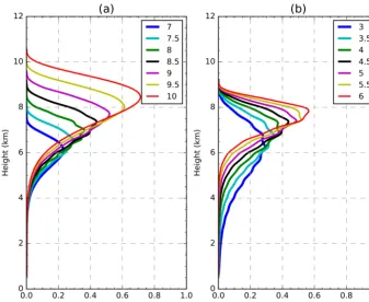
whereS(z)is the mass eruption rate distribution function,z is the altitude above the vent,his the top height of the erup-tive column, andAandλare two dimensionless parameters. Figure 1 shows the sensitivity of the vertical emission pro-file to different values of handA. It is important to recall that h not only controls the maximum height of the erup-tive column, but also the total mass emitted (Fig. 1a). Pa-rameterAdoes not modify the total amount of mass being emitted but significantly affects the level at which the maxi-mum emission takes place (Fig. 1b), which can significantly affect the posterior evolution of the ash plume, particularly for cases in which there is strong vertical wind shear. The parameterλis a measure of how concentrated the emission is around the maximum (not shown). A previous sensitivity test (Osores, 2018) has shown that the two FALL3D model parameters that most affect the model results are the eruption column heighth and the parameter Ain the Suzuki distri-bution. For this reason, these two parameters will be used in the following sections to define the ETKF–FALL3D system experiments. The sensitivity of the FALL3D model to these
parameters in terms of the deposit has been documented by, e.g., Scollo et al. (2008).
2.2 The ETKF–FALL3D system
In operational applications, data assimilation is implemented sequentially to provide an estimation of the state of the sys-tem at a series of times in the so-called “data assimilation cycle”. Each data assimilation cycle consists of two steps: a first step in which the numerical model is used to provide an a priori estimation or forecast of the state of the system and its uncertainty, followed by a second step in which the prior estimation is combined with observations (which are also considered uncertain) to obtain a posterior estimation or analysis. These two steps are repeated sequentially in order to propagate forward in time information from past observa-tions.
Let us assume that the state of a system at timetis repre-sented by a state vectorxt that, in our particular case, con-sists of the values of ash concentration at each model grid point and for each particle class. In other words,xt is a col-umn vector withnelements,nbeing the total number of state variables in the FALL3D model (i.e., the total number of grid points times the number of particle bins). For parameter es-timation, model parametersθ, e.g., those defining the char-acteristics of the source term, are also considered part of the state of the system and are thus assumed uncertain. For the sake of simplicity, we limit the FALL3D source term parame-ters to the eruption column heighthand theA-Suzuki param-eter, but the methodology that follows can easily be extended to any other set of model input parameters. The augmented state vector st at time t is defined as the concatenation of the state vectorxtand the (time-dependent) estimated model parametersθ; that is, st = [xt, θt] is a column vector with ns=n+2 elements.
In the ensemble Kalman filter the time-dependent uncer-tainty in the state variables and parameters is estimated using a Monte Carlo approach through an ensemble of augmented states. Let us assume that we start at timet−1 with an en-semble of initial conditions and model parameters. Then, our forecast of the state of the system at timet is obtained by integrating in time the FALL3D model for each ensemble member:
sf (i)t =Mt
Figure 1.Vertical mass distribution for different(a)eruptive column top heights and(b)ASuzuki parameters.
matrix estimated from the ensemble of forecasts:
sft =k−1 k
X
i=1
sf (i)t , (3)
Pft =(k−1)−1Sft Sft T, (4) wheresft is the ensemble forecast mean,Pft is the ensem-ble forecast covariance matrix (a square matrix of dimension ns×ns), andSft is the ensemble forecast perturbation matrix whoseith column is computed asSf (i)t =sf (i)t −sf (i)t .
Note that the integration of the ensemble in time propa-gates the uncertainty on the initial conditions and parame-ters at time t−1 into the future in order to provide a time-dependent estimation of the forecast uncertainty. This is a key feature that makes these methods particularly appealing for the estimation of uncertain model parameters (e.g., Aksoy et al., 2006; Ruiz et al., 2013) and for an accurate quantifi-cation of concentration. At the analysis step a set of observa-tions is available that is related to the true state of the system by the following expression:
yt =H xtruet
+t, (5)
whereytis anm-sized column vector containing the value of themobservations at timet, andxtrueis the true model state (assumed to be unknown).His a (usually nonlinear) trans-formation that maps the state variables (i.e., ash concentra-tions for different particle sizes) into the observed quantities
(e.g., cloud column mass load), and the vector represents the error in the observations. This error is typically assumed to be a zero-mean Gaussian random variable with covariance matrixR(dimensions ofm×m). The errors in the observa-tions are assumed to be uncorrelated in time and indepen-dent of the state of the system. Under these assumptions, the information provided by the forecast and the observations can be combined to obtain an estimation of the augmented state that minimizes the root mean square error (RMSE) with respect to the unknown truth (e.g., Kalnay, 2003; Carrassi et al., 2018):
sat =sft +Pft HtT(HtPftHTt +R) −1yf
t −H(x f t )
, (6)
wheresat is the a posteriori estimation of the augmented state (i.e., the analysis), andHtis the tangent linear of the observa-tion operator. The factorPftHTt (HtPft HTt +R)−1is usually referred to as the Kalman gain. The Kalman filter equations also provide a way to estimate the uncertainty of the analy-sis. After the assimilation of the observations, the augmented state covariance matrix is updated to
Pat =(I−KHt)Pft , (7)
wherePa
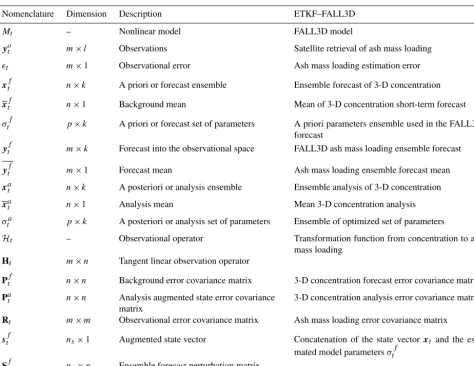
Table 1.Summary of the notation used in the paper, with the nomenclature for the ETKF method and its correspondence to the experiments discussed in this work. Here,nis the total number of grid points times the number of particle classes in the FALL3D model,mis the number of observations at timet,pis the number of parameters, andkis the number of ensemble members.
Nomenclature Dimension Description ETKF–FALL3D
Mt – Nonlinear model FALL3D model
yot m×l Observations Satellite retrieval of ash mass loading
t m×1 Observational error Ash mass loading estimation error
xft n×k A priori or forecast ensemble Ensemble forecast of 3-D concentration
xft n×1 Background mean Mean of 3-D concentration short-term forecast
σtf p×k A priori or forecast set of parameters A priori parameters ensemble used in the FALL3D forecast
yft m×k Forecast into the observational space FALL3D ash mass loading ensemble forecast
yft m×1 Forecast mean Ash mass loading ensemble forecast mean
xat n×k A posteriori or analysis ensemble Ensemble analysis of 3-D concentration
xat n×1 Analysis mean Mean 3-D concentration analysis
σta p×k A posteriori or analysis set of parameters Ensemble of optimized set of parameters
Ht – Observational operator Transformation function from concentration to ash mass loading
Ht m×n Tangent linear observation operator
Pft n×n Background error covariance matrix 3-D concentration forecast error covariance matrix
Pat n×n Analysis augmented state error covariance matrix
3-D concentration analysis error covariance matrix
Rt m×m Observational error covariance matrix Ash mass loading error covariance matrix
sft ns×1 Augmented state vector Concatenation of the state vectorxt and the esti-mated model parametersσtf
Sft ns×ns Ensemble forecast perturbation matrix
mean and covariance matrix equal to Pat. These equations can be difficult to solve explicitly for high-dimensional sys-tems due to the large size ofPt andRt, but several methods have been proposed to address this issue and to implement the ensemble Kalman filter in high-dimensional systems. In the present work, we use the ETKF approach, which solves the ensemble Kalman filter equations in a subspace defined by the ensemble members. Details about the equation that arises from this particular implementation can be found in Hunt et al. (2007), but a summary is given in Appendix A. Table 1 also presents a summary of the notation and dimen-sions associated with the different quantities previously dis-cussed. One of the main advantages of this approach is that finding the analysis ensemble mean requires inverting ak×k matrix, which is significantly cheaper than inverting then×n matrix for the case in whichkn(which is usually the case for high-dimensional applications of the filter).
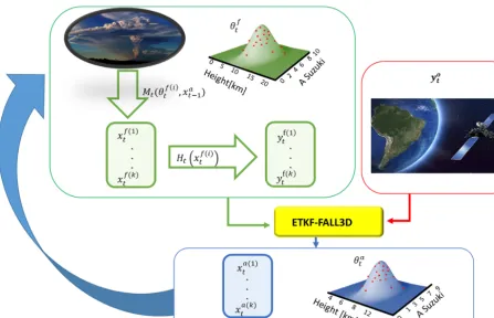
The process is schematically shown in Fig. 2. The cycle starts with an estimation of the mean parameters;
assum-ing they have a Gaussian distribution,krandom samples are taken. Each parameter sample is used in one of the ensemble members integrated with the dispersion model. When an ob-servation is available, it is combined with the ensemble fore-casts using the ETKF equations. From this combination an ensemble of analysis is obtained with a set of optimized pa-rameters that also has a Gaussian distribution. Then the next cycle starts from the ensemble of analysis and the set of opti-mized parameters to produce a new ensemble forecast. When a new observation is available, the assimilation method is ap-plied, and the cycle continues.
3 ETKF–FALL3D experimental setup
Figure 2.ETKF–FALL3D data assimilation system scheme for volcanic ash.
run. Observations are simulated from the nature run and then assimilated with the ETKF–FALL3D system. The June 2011 Puyehue-Cordón Caulle eruption (Osores et al., 2012; Collini et al., 2013) has been selected for the generation of the nature run.
3.1 Ash mass loading observation simulations
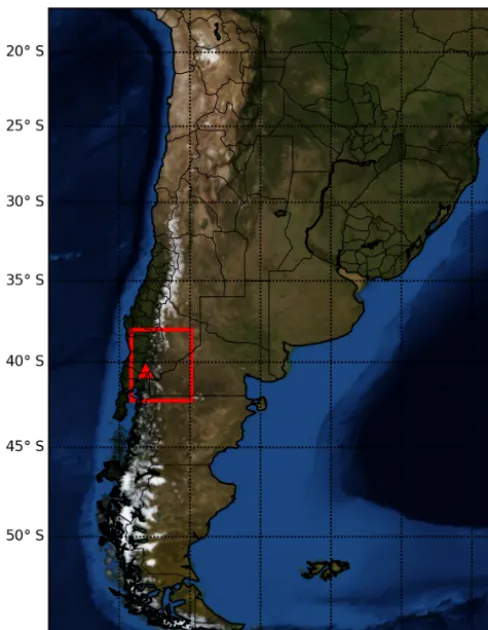
The nature run and observation simulation begin at 18:00 UTC on 4 June 2011 and last for 10 d up to 00:00 UTC on 15 June, covering the domain shown in Fig. 3 with a model horizontal resolution of 0.23◦ and a vertical resolu-tion of 200 m. The model top is located at 20 km above the ground. The volcanic vent is located at 40.52◦S–72.15◦W at an altitude of 1420 m a.s.l.
The particle total grain size distribution (GSD) is repre-sented by 12 classes with diameters between 2 mm (−1φ) and 1 µm (10φ) and densities ranging from 400 for the larger particles to 2100 kg m−3 for the smaller ones (Bonadonna
et al., 2015). The vertical distribution of the source is param-eterized using the Suzuki scheme consideringλ=5, the set-tling velocity model is that of Ganser (Ganser, 1993), and the vertical and horizontal turbulent diffusion are parameterized by the similarity (Ulke, 2000) and Community Multiscale Air Quality (CMAQ) (Byun and Schere, 2006) schemes, re-spectively. The meteorological fields are obtained from the Global Forecasting System (GFS) analysis with a horizontal
resolution of 0.5◦, a temporal resolution of 6 h, and 27 con-stant pressure vertical levels.
The simulated observations represent ash mass column load (vertically integrated ash mass per unit area) estimates retrieved from satellite radiances (e.g., Prata and Prata, 2012; Francis et al., 2012; Pavolonis et al., 2013). Simulations of satellite retrievals are chosen since these observations are available almost globally and have a high spatial and tem-poral resolution, making them particularly appealing for the implementation of operational data assimilation systems. To represent some of the limitations of current satellite-based ash mass load retrievals, the simulated observations are avail-able only where the true load values are between 0.2 and 10 g m−2. The lower bound approximately corresponds to the minimum mass load that can be retrieved by state-of-the-art algorithms. Retrievals usually cannot estimate mass loads over the upper bound because the optical thickness of the corresponding ash plume is too high (e.g., Wen and Rose, 1994; Prata and Prata, 2012; Pavolonis et al., 2013). The ob-servational error is assumed to have a random Gaussian dis-tribution, with a standard deviation of 0.15 of the ash mass load.
Figure 3.Domain used in the ETKF–FALL3D sensitivity tests (red square).
the ash cloud. Two nature runs were generated to evaluate the ETKF–FALL3D system: one with constant emission profiles and another with time-varying emission profiles.
3.1.1 Constant emission profile
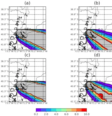
This nature run simulation considers a source term that re-mains constant during the entire simulated period, with an eruption column height of 8.5 km above the vent and anA Suzuki parameter of 5.5 (Fig. 4). Figure 5a and c show the ash mass loading from the nature run and the observation simulation on 7 June at 12:00 UTC for illustrative purposes. The addition of observational error to the nature run does not significantly affect the spatial distribution or the location and intensity of the maximum concentration. The number of available observations (which depends on the thresholds de-scribed in the previous section) is time-dependent (ranging from 27 to 52 grid point observations) and, in this partic-ular case, is primarily affected by the atmospheric circula-tion, which produces variations in the 3-D ash concentration within the model domain.
Figure 4.Nature run parameter time series for the constant (solid lines) and variable emission profiles (dashed lines) forh (black lines) andASuzuki (red lines).
3.1.2 Variable emission profile
In this experiment, h and A Suzuki are time-dependent (Fig. 4). In order to represent a realistic variability of the source parameters, theh evolution corresponds to the esti-mated heights during the 2011 Puyehue-Cordón Caulle erup-tion (Osores et al., 2014). Since theASuzuki parameter can-not be directly estimated, the evolution of this parameter is simulated using an auto-regressive model (Fig. 4).
In Fig. 5b and d, the ash mass loading fields for 7 June at 12:00 UTC from the nature run and the observation simula-tion are shown. As has been shown for the constant parame-ter case, the observational error does not significantly affect the spatial distribution of the plume. In this experiment, the number of observations assimilated depends on the emission profile as well as the wind field, and it can range from 15 (on 11 June at 06:00 UTC) to 86 (on 11 June at 18:00 UTC). 3.2 Data assimilation experimental setup
pa-Figure 5.Ash mass loading on 7 June at 12:00 UTC for(a)the nature run with constant parameters,(c)the run with observational error and constant parameters, the(b)nature run with time-dependent parameters, and(d)the run with observational error and time-dependent parameters. Ash mass loading values outside the 0.2–10.0 g m−2interval are in grey.
rameters, the ensemble spread is inflated back to its origi-nal value after assimilating the observations (similar to the conditional inflation approach of Aksoy et al., 2006). This is equivalent to assuming that the parameter uncertainty is time-independent, thus preventing the parameter ensemble spread from collapsing. Covariance localization is usually required to reduce the impact of spurious correlation that re-sults from the use of small ensemble sizes. The estimation of small correlations (e.g., between locations that are far apart from each other) is usually strongly affected by sampling noise; this is why estimated covariances are usually forced to decay with distance. Since the domain used in the data as-similation experiments is small, the impact of spurious corre-lations between distant grid points is less significant. For this reason, no covariance localization is used in the estimation of the state variables or the parameters. However, is impor-tant to keep in mind that if the system is extended to larger
domains, using covariance localization will highly improve its performance.
range. The physically meaningful range for model parame-ters is set to 0–20 km and 0–15 forhandASuzuki, respec-tively. The number of grid points and ensemble members with estimated concentrations below −1.0×10⁻⁴g m−3 is usually below 15 % of the grid points and ensemble mem-bers for which the concentration has been updated. This pro-portion decreased with increasing ash concentration as well as with ensemble spread. Estimated parameters for individ-ual ensemble members fall outside the physical meaningful range less than 10 % of the times, also depending on how close to the boundaries the true parameters are and how large the parameter ensemble spread is.
One of the main hypotheses of the Kalman filter is that state variables and parameters are approximately linearly correlated with the observations. This is not true for the h parameter since in the Mastin et al. (2009) emission scheme the source strength is proportional to the fourth power ofh. For this reason, instead of estimating h, we estimate h4 so that the estimated parameter is more linearly correlated with the observations.
In this work, several experiments are performed to study the convergence of the filter and its sensitivity to some key parameters. Two experiments are performed using the con-stant parameter nature run to assess filter convergence. The first experiment starts with source parameters that are higher than the true value and will be referred to as CONSTANT-UPPER; the second starts with an underestimation of the source parameters and will be referred to as CONSTANT-LOWER. The initial parameter spread forh andASuzuki is 500 and 0.5 m, respectively, and is the same for both periments. These experiments are compared against an ex-periment in which parameters remain constant at their initial value (CONSTANT-NOEST) and against an experiment in which the parameters are constant and their ensemble mean is equal to the true value (CONSTANT-TRUE).
The second set of experiments is based on the nature run with time-dependent parameters. An estimation experiment that uses the same parameter ensemble spread as in the pre-vious experiments is performed and will be referred to as the CONTROL experiment. To evaluate the impact of per-forming parameter estimation in the time-dependent param-eter context, an experiment in which the paramparam-eters are kept constant at the time average of the true parameters is also presented (CONTROL-NOEST).
To quantify the sensitivity of the ETKF–FALL3D system to the parameter ensemble spread, two additional experi-ments are performed: one in which the ensemble spread is larger than in the CONTROL experiment (HI-SPREAD), for which the spread inhandASuzuki is 2000 and 4 m, respec-tively, and another experiment in which the ensemble spread is lower than in the CONTROL run (LOW-SPREAD), for which the spread in h andASuzuki is 100 and 0.1 m, re-spectively. All the other configuration settings are as in the CONTROL experiment.
To explore the impact of modifying the ensemble size, an experiment with ensemble sizes of 8 8) and 16 (ENS-16) is presented for which all other configuration settings are equal to the CONTROL run experiment. Finally, the impact of observation error is assessed in two experiments with ob-servation errors that are 30 (OBS-30) and 40 % (OBS-40) of the true total mass concentration. All presented data assimi-lation and parameter estimation experiments are summarized in Table 2, including the statistical properties of the initial parameter ensemble. Finally, a set of simulation experiments is carried out using a larger domain to evaluate the impact of the optimized parameters upon the simulation of the ash cloud farther from the vent.
3.3 Performance metrics
The evaluation of the FALL3D-ETKF system is achieved by comparing the 3-D ash concentration forecast (and analysis) against the nature run and also by measuring the consistency between the estimated and the actual forecast uncertainties. The comparison is based on the RMSE, error bias, and the ensemble spread of either the forecast or the analysis, which are given by the following expressions:
RMSE=
v u u tN−1
N
X
i=1
xf,i−xt,i2, (8)
BIAS=N−1 N
X
i=1
xf,i−xt,i, (9)
SPREAD=
v u u tN−1
N
X
i=1 k−1
k
X
j=1
x(j )f ,i−xf,i
2 !
, (10)
wherexf,iis either the forecast or analysis ensemble mean ash concentration at time and locationi andx(j )f,i, andxt,i represents their corresponding values for thejth ensemble member and the nature run, respectively. Spatial or temporal averages are obtain by summing overi.
4 Results
4.1 Constant emission profile experiments
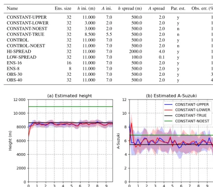
Table 2.Summary of the main parameters that distinguish the different experiments described in the text.
Name Ens. size hini. (m) Aini. hspread (m) Aspread Par. est. Obs. err. (%)
CONSTANT-UPPER 32 11.000 7.0 500.0 2.0 y 15
CONSTANT-LOWER 32 3.000 2.0 500.0 2.0 y 15
CONSTANT-NOEST 32 3.000 2.0 500.0 2.0 n 15
CONSTANT-TRUE 32 8.500 5.5 500.0 2.0 n 15
CONTROL 32 11.000 7.0 500.0 2.0 y 15
CONTROL-NOEST 32 11.000 7.0 500.0 2.0 n 15
HI-SPREAD 32 11.000 7.0 2000.0 4.0 y 15
LOW-SPREAD 32 11.000 7.0 100.0 0.1 y 15
ENS-16 16 11.000 7.0 500.0 2.0 y 15
ENS-8 8 11.000 7.0 500.0 2.0 y 15
OBS-30 32 11.000 7.0 500.0 2.0 y 30
OBS-40 32 11.000 7.0 500.0 2.0 y 40
Figure 6.Optimized parameters as a function of time in the UPPER (blue line), LOWER (red line), TRUE (black line), and NOEST (green line) experiments. The shading surrounding the UPPER and CONSTANT-LOWER estimated values represents±1 standard deviation;(a)hparameter and(b)ASuzuki parameter.
true parameter, indicating that the parameter estimation tech-nique is robust in finding the correct values of parameters regardless of ensemble initialization. As observed in Fig. 6, both parameter estimation experiments tend to sub-estimate the values ofhand to slightly overestimate the values ofA Suzuki. Figure 6 also shows the parameter ensemble spread. In these experiments, the ensemble almost always contains the true parameter value, meaning that the parameter uncer-tainty is well captured by the ensemble. However, it should be noted that, in these experiments, the ensemble spread of the model parameters is prescribed a priori to a value that may not be the optimal one under different conditions (e.g., if the optimal parameters are time-dependent or if other sources of uncertainty, like errors in the atmospheric circulation, are present). Sensitivity experiments to the parameter ensemble spread will be discussed in the following sections.
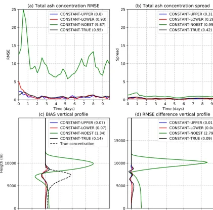
shows the spatially averaged ash concentration ensemble spread. One way to assess if the current parameter ensemble spread is well tuned is to compare the ash concentration fore-cast error and spread. If these are similar then we can assume that our uncertainty is well represented in the ensemble. In this case, the uncertainty in the ash concentration is mainly associated with the uncertainty in the source parameters. As observed, the spread values are close to the RMSE values in Fig. 7a, which indicates that after convergence of the param-eters, the ensemble spread closely represents the magnitude of the errors.
Figure 7c shows the horizontal and time-averaged error bias for the total ash concentration as a function of height. The first 2 d have been excluded because they are considered part of the spin-up time of the filter. This figure shows that biases associated with the estimation experiments are much lower than for the CONSTANT-NOEST experiment, show-ing once again the advantage of optimizshow-ing the source pa-rameters. The CONSTANT-UPPER, CONSTANT-LOWER, and CONSTANT-TRUE experiments show a small system-atic underestimation of the maximum concentrations and an overestimation above and below the location of the maxi-mum. Note that the bias is slightly lower in the parameter es-timation experiments with respect to the CONSTANT-TRUE experiment.
The fact that a biased parameter ensemble (i.e., the under-estimation ofhobserved in Fig. 6a) produces a less biased es-timation of ash concentrations (Fig. 7c) may be related to the nonlinear relationship betweenhand the total mass emission at the source. Since the emitted mass depends onh4, positive perturbations inhare associated with a much larger emission rate and are thus farther from the observations than ensem-ble members with negative perturbations inh. This creates a bias in the estimation of the concentrations because, even if the ensemble is centered at the truehvalue, positive pertur-bations are farther from observations than the negative ones, and therefore the ensemble mean tends to overestimate centrations. ETKF tries to compensate for this effect by con-verging to a slightly biased parameter set, which reduces the error bias and the RMSE.
As observed in Fig. 7d, the analysis error in ash concentra-tion is below the forecast error. This indicates that the ETKF method is efficient in reducing the error in the 3-D concentra-tion field based on the informaconcentra-tion provided by a 2-D obser-vation. This is a remarkable result in a context in which most observations are 2-D, whereas operational requirements are 3-D. This finding will be the basis for using the analysis as a better diagnostic of the state of the plume to improve the casts. The reason behind this lies in the structure of the fore-cast error covariance matrix, which is estimated from the en-semble of forecasts. This matrix contains information about the covariances between mass loading (which is the observ-able quantity) and the concentration at different heights from which the mass loading is obtained and which are not directly observed. In this work, reliable covariances between 3-D ash
concentrations and mass loadings are obtained by taking into account the uncertainties associated with the source parame-ters.
4.2 Time-dependent emission experiments
These experiments use the observations simulated from the nature run with time-varying parameters (Fig. 4). The pa-rameter ensemble is initialized with a mean hof 11 km, a mean A Suzuki of 7, and standard deviations of 0.5 and 2.0 km, respectively. Figure 8 shows the evolution in time of the optimized parameter ensemble as well as their corre-sponding true values, showing a good agreement. The esti-mation ofhseems to be particularly accurate and can detect rapid variations in the eruptive column height, with RMSE values lower than 200 m throughout the experiment. For the ASuzuki parameter, the time evolution is not reproduced so accurately. There are also two sudden jumps in the estima-tion ofASuzuki, indicating a less well-constrained parame-ter value. These differences in the behavior of the estimated handASuzuki may be due to the higher sensitivity of the ash distribution to the eruptive column height in comparison with theASuzuki parameter. The jumps in the estimatedA Suzuki occur during periods of fast changes inh, suggesting that whenhis not well estimated,ASuzuki may be modified in an attempt to compensate for errors inh.
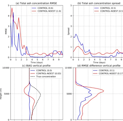
Figure 9 shows the RMSE of the forecast for the 3-D to-tal ash concentration. Errors in this case vary strongly with time, with larger errors corresponding to the instants in which his larger, leading to stronger ash mass emission at the vent and consequently larger ash concentrations in the surround-ings of the vent. The ensemble spread (Fig. 9b), although smaller than the error (indicating an under-dispersive ensem-ble), changes accordingly with more spread during the peri-ods in which the emission is higher. These changes in the en-semble spread are a consequence of the relationship between hand mass emission at the vent. Sincehdeviations from the ensemble mean are almost time-independent, the associated departures in mass emission are larger during the periods of higherh, leading to a larger spread in the concentration field. Figure 9d shows the spatially averaged reduction in the RMSE for the total ash concentration between the forecast and the analysis. The RMSE is reduced between the forecast and the analysis at almost all vertical levels, indicating that the vertical covariance structure between mass loadings and ash concentrations at different levels is well estimated, lead-ing to accurate 3-D ash concentration estimations.
Figure 7. (a)Spatially averaged forecasted total ash concentration RMSE,(b)spatially averaged forecasted total ash concentration ensemble spread, (c)spatially averaged forecasted total ash concentration bias, and (d)the difference between the 6 h forecast and analysis total ash concentration RMSE for the CONSTANT-UPPER (blue line), CONSTANT-LOWER (red line), CONSTANT-TRUE (black line), and CONSTANT-NOEST (green line) experiments. Panels(a),(b), and(c)are computed from the 6 h ensemble forecast (all values: 10−3g m−3).
time-dependent parameters. Figure 9 shows that the forecast RMSE and bias in the 3-D ash concentration are almost al-ways larger in the CONTROL-NOEST experiment with re-spect to the CONTROL experiment. The error in the CON-TROL and CONCON-TROL-NOEST experiments becomes simi-lar around day 3 and after day 8 because at those times in-stants the source parameters are close to each other (Fig. 8). Moreover, the ensemble spread for the CONTROL-NOEST experiment is almost constant in time and, because of that, changes in the forecast uncertainty are not captured (Fig. 9b). This is because time variations in the ensemble spread are mainly associated with changes in the mean values of pa-rameters. These experiments suggest that performing data
as-similation for the estimation of 3-D ash concentrations is not sufficient to properly constrain 3-D ash concentration val-ues and that source parameters also have to be taken into ac-count, particularly close to the source where these parameters rapidly impact concentrations.
par-Figure 8.Optimized parameters as a function of time in the CONTROL (blue line) and CONTROL-NOEST (red line) experiments. The shading surrounding the estimated values represents±1 standard deviation;(a)hparameter and(b)ASuzuki parameter. The black line indicates the value of the parameters in the true run.
ticular time. Note that data assimilation is being performed to correct the 3-D ash concentrations in both experiments.
4.3 Sensitivity experiments
This section discusses the sensitivity of the analysis and the forecast to the parameter ensemble spread, the ensemble size, and the observation uncertainty. The purpose is to identify the potentially more important tuning parameters for the op-timization of the system and how robust the system is with respect to errors in observations, which are known to exist in satellite-based ash mass loading estimations.
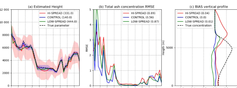
To explore the sensitivity to the parameter ensemble spread, the experiments CONTROL, HI-SPREAD, and LOW-SPREAD with different parameter spreads (Table 2) are compared. Figure 11 shows the estimated h obtained in these experiments as well as the total ash concentration RMSE and bias. As observed, the CONTROL experiment gives a more accurate estimation of h and the minimum RMSE and bias. When the parameter ensemble spread is larger than in the CONTROL experiment, parameter values are systematically underestimated. As previously discussed, this can be explained by the nonlinear dependence between hand the total emitted mass. However, what is relevant from this experiment is that increasing the ensemble spread de-grades the quality of the estimation and increases the im-pact of nonlinearities. Higher dispersion in hincreases the magnitude of positive h perturbations, leading to a larger error bias, particularly above and below the maximum con-centration (Fig. 11c). In the case of the LOW-SPREAD ex-periment, results are closer to the CONTROL experiment. However, this experiment shows a slower convergence with larger h estimation errors during the first days of the
ex-periment. Slower convergence or a lack of convergence is expected when the parameter uncertainty is underestimated. In this case, the ETKF does not allow for large corrections in the parameter values based on the observations, basically because the error in the parameters is assumed to be small. These experiments show that the system is particularly sensi-tive to the parameter ensemble spread that has to be specified a priori. Moreover, in these idealized experiments, the opti-mal parameter ensemble spread is determined by the uncer-tainty in the observations and with no information regarding the changes in the true parameters in time.
Figure 9.As in Fig. 7 but for the experiments CONTROL (blue line) and CONTROL-NOEST (red line; all values: 10−3g m−3).
effective low dimensionality is reinforced by the fact that the domain is small and close to the source, and, because of that, the ash concentration at most grid points is strongly corre-lated with the value of the uncertain source parameters.
The last sensitivity experiment looks into the issue of ob-servation errors in satellite retrievals of mass loadings. In the experiments presented so far, the standard deviation of the observation errors has been assumed to be 15 % of the mass loading in the nature run. However, in real cases, uncertain-ties associated with mass loading estimations can be larger than that. Two additional experiments are performed to ex-plore the impact of the magnitude of the observation errors on the estimation of source parameters and total ash con-centrations with an observation standard deviation of 30 % (OBS-30) and 40 % (OBS-40) of the true mass loading value. Results from these experiments are presented in Fig. 13. As
Figure 10. (a)Nature run ash concentration at flight level 200 (shaded, 10−3g m−3);(b)as in(a)but for the 6 h forecast of ash concentration initialized from the CONTROL analysis experiment;(c)as in(b)but for the CONTROL-NOEST experiment, corresponding to the 12th assimilation cycle.
Figure 11. (a)Estimatedhas a function of time for the HI-SPREAD (red line), CONTROL (blue line), and LOW-SPREAD (green line). The shading surrounding the estimated values represents±1 standard deviation, and the black dashed line indicates the true parameter value. (b)Spatially averaged total ash concentration 6 h forecast RMSE as a function of time (10−3g m−3). Line color code as in(a).(c)Temporally averaged 6 h forecast bias as a function of height (10−3g m−3). Line color code as in(a).
4.4 Ash concentration simulations in an extended domain simulation
The experiments discussed so far have been performed in a relatively small domain surrounding the vent. In most appli-cations, however, it is expected that forecasts over larger do-mains are required. In this section, we explore the adequacy of the parameter estimation approach to generate a good esti-mation of ash dispersion over larger domains in an idealized context in which the atmospheric flow is perfectly known. For this purpose, a nature simulation over a larger domain is performed. This nature run is forced with the same evo-lution as parameters of the time-dependent parameter nature run and spanning the same period.
Figure 12.As in Fig. 11 but for the experiments CONTROL, ENS-16, and ENS-8.
Figure 13.As in Fig. 11 but for the experiments CONTROL, OBS-30, and OBS-40.
nature is not or vice versa, respectively). We note that both ash clouds are very close to each other, even far from the source, indicating that the estimated parameters are sufficient for the reconstruction of the ash plume in this ideal case.
To see if the CONTROL-LD experiment can be used to initialize short-range ash concentration forecasts over the larger domain a forecast is initialized using the CONTROL-LD ash concentrations as initial conditions and the CON-TROL parameter ensemble mean as source parameters. Note that in this case, parameters remain constant during the fore-cast. Figure 14a and b show the 12 and 24 h forecast lead times initialized on 7 June at 12:00 and 00:00 UTC, respec-tively. There is a good agreement between forecasts and the nature run. For larger lead times there are more false alarms and misses as expected. This suggests that initializing a fore-cast from a long run forced with the optimized parameters can be a cost-effective strategy to generate short-lead-time ash concentration forecasts over a relatively large domain.
Although these results are encouraging, it should be taken into account that in more realistic situations, other sources of uncertainty (e.g., uncertainty in the flow or model errors) can significantly affect the evolution of the ash plume far from the source. In this case, the forecast quality can suffer from the estimation of the 3-D ash concentration over the entire domain based on the assimilation of mass loading observa-tions.
5 Summary and conclusions
Figure 14.Ash mass loading above 0.2 g m−2comparison between the ensemble mean optimized parameter run, the 12 h forecast, and the 24 h forecast against the nature run over a larger domain, verifying on 8 June at 00:00 UTC (see the text for details).
time variability of the ensemble spread is mainly associated with the relationship between column height and emitted mass.
Sensitivity experiments have been conducted to investigate how the parameter ensemble spread, the ensemble size, and the observation errors affect the results. The parameter en-semble spread produces a significant impact on the quality of the estimated concentrations and parameters. Larger ensem-ble spreads lead to stronger biases, both in concentrations and parameters, whereas lower ensemble spreads produce an overconfident ensemble and slower converge rates that de-grade the estimation results. It is important to note that the optimal parameter ensemble spread can depend on the time variability of the estimated parameters and other sources of uncertainty like errors present in the observations and the model. The sensitivity to the ensemble size revealed that, even for this low-dimensional estimation problem, ensemble sizes up to 32 members show some improvement with re-spect to ensembles of 16 and 8 members, although the impact of increasing the ensemble size is smaller than the impact as-sociated with changes in the parameter ensemble spread.
The sensitivity to the observation errors shows a particular behavior, with an increase in systematic errors both in the pa-rameters and in the concentrations with increasing observa-tional errors. When observation errors reach 40 % of the true ash loadings, the estimated parameters fail to converge dur-ing the first days of the experiment, leaddur-ing to significantly larger errors in the ash concentration forecasts.
The experiments presented in this work are limited to a small domain surrounding the vent. Experiments on a larger domain show that the optimized parameters can be used to force an ash dispersion simulation that can reproduce the ash cloud properties far from the vent as long as the atmospheric circulation is accurately known. These simulations can be used to initialize ash dispersion forecasts over a larger do-main as a computationally cheaper alternative to running a data assimilation system with covariance localization over a large domain.
The experiments discussed in this work assume a perfect model and a perfect meteorological forcing. In real-life ap-plications, imperfections in the model and the forcing have a significant impact on the quality of ash dispersion fore-casts. Previous works have shown that parameter estimation can be successfully performed in the presence of multiple sources of model error (e.g., Ruiz and Pulido, 2015). Prelim-inary experiments introducing errors in the meteorological forcing suggest that the current system provides a robust es-timation of the source parameters in the presence of wind uncertainty. However, this aspect should be further analyzed in future studies.
formulation among the most important; (c) the assessment of the skill of the system in more realistic scenarios using real observations; (d) a better representation of the uncer-tainty associated with observations, considering possible co-variances among observations as well as systematic biases in the observations; (e) the development of techniques that can converge to the optimal parameter ensemble spread based on the information provided by the observations (e.g., Miyoshi, 2011); and (f) the implementation of nonlinear assimilation approaches (e.g., Bocquet et al., 2010) that can better handle non-Gaussian error distributions and nonlinear relationships between the model parameters and the observable quantities.
Appendix A: ETKF formulation
A brief description of the ensemble transform Kalman fil-ter equations are provided here. See Hunt et al. (2007) for a derivation of the equations as well as for a detailed discus-sion of the method. The ETKF approach solves the Kalman filter equations in the subspace defined by the ensemble per-turbations (i.e., the departures of individual members from the ensemble mean). Under this framework, the update in the ensemble mean can be expressed as a linear combination of the forecast perturbations as follows:
sat =sft +Sft wat, (A1)
wherewat is a vector of weights of dimensionkcomputed as
wat =fPat(Yft)TR−1
yt−ytf
. (A2)
Here, Yft is the ensemble perturbation matrix in obser-vation space, whose ith column is computed as Yf (i)t = H(xf (i)t )−H(xft ), andfPat is the analysis covariance matrix
in the subspace spanned by the ensemble members and is computed as
f
Pat =h(k−1)I+(Yft )TR−1Yfti −1
, (A3)
withIbeing the identity matrix of sizek×k. The analysis en-semble perturbations are obtained as an optimal linear com-bination of the background ensemble perturbations:
Sat =Sft Wat, (A4)
and the weight matrixWat is computed as Wat =(k−1)ePat
1/2
. (A5)
Finally, the analysis ensemble is obtained as the sum of the analysis ensemble mean and the analysis perturbations:
sa(i)t =sat +Sa(i)t . (A6)
Note also that, in this implementation, the tangent lin-ear observation operator H is not applied explicitly since HtPft HTt is approximated by Y
f t (Y
f
Author contributions. All authors conceived the presented idea, de-signed the experiments, and conducted the analysis of the results. AF provided guidance on the use of the FALL3D model, and JR provided guidance on the implementation of the ensemble trans-form Kalman filter. SO and JR developed the code and pertrans-formed the computations. All the authors contributed to paper writing and approved the final paper.
Competing interests. The authors declare that they have no conflict of interest.
Acknowledgements. The authors would like to acknowledge the editor and the two reviewers for their comments and suggestions that helped to significantly improve the quality of the paper. Sim-ulations were made with the high-performance computing clusters at the Barcelona Supercomputing Center, Spain, and CIMA/UBA-CONICET, Argentina.
Financial support. Soledad Osores has been founded by a CONICET-CONAE doctoral fellowship. This work has been par-tially funded by the H2020 Center of Excellence for Exascale in Solid Earth (ChEESE) under grant agreement 823844, by grants PICT2014-1000 and PICT2017-2233 from the Argentinian Na-tional Agency for Scientific Research Promotion, and by grants UBACyT 2014 and 2018 from the University of Buenos Aires.
Review statement. This paper was edited by Josef Koller and re-viewed by Fei Lu and one anonymous referee.
References
Aksoy, A., Zhang, F., and Nielsen-Gammon, J. W.: Ensemble-based simultaneous state and parameter es-timation with MM5, Geophys. Res. Lett., 33, L12801, https://doi.org/10.1029/2006GL026186, 2006.
Bocquet, M., Pires, C. A., and Wu, L.: Beyond Gaussian Statistical Modeling in Geophysical Data Assimilation, Mon. Weather Rev., 138, 2997–3023, https://doi.org/10.1175/2010MWR3164.1, 2010.
Bonadonna, C., Cioni, R., Pistolesi, M., Elissondo, M., and Bau-mann, V.: Sedimentation of long-lasting wind-affected volcanic plumes: the example of the 2011 rhyolitic Cordón Caulle erup-tion, Chile, B. Volcanol., 77, 13, 2015.
Byun, D. and Schere, K. L.: Review of the governing equations, computational algorithms, and other components of the Models-3 Community Multiscale Air Quality (CMAQ) modeling system, Appl. Mech. Rev., 59, 51–77, 2006.
Carrassi, A., Bocquet, M., Bertino, L., and Evensen, G.: Data assimilation in the geosciences: An overview of methods, issues, and perspectives, WIREs Clim. Change, 9, e535, https://doi.org/10.1002/wcc.535, 2018.
Chai, T., Crawford, A., Stunder, B., Pavolonis, M. J., Draxler, R., and Stein, A.: Improving volcanic ash predictions with
the HYSPLIT dispersion model by assimilating MODIS satellite retrievals, Atmos. Chem. Phys., 17, 2865–2879, https://doi.org/10.5194/acp-17-2865-2017, 2017.
Clarkson, R. J., Majewicz, E. J., and Mack, P.: A re-evaluation of the 2010 quantitative understanding of the effects volcanic ash has on gas turbine engines, P. I. Mech. Eng. G.-J. Aer., 230, 2274– 2291, 2016.
Collini, E., Osores, M. S., Folch, A., Viramonte, J. G., Villarosa, G., and Salmuni, G.: Volcanic ash forecast during the June 2011 Cordón Caulle eruption, Nat. Hazards, 66, 389–412, 2013. Costa, A., Macedonio, G., and Folch, A.: A three-dimensional
Eu-lerian model for transport and deposition of volcanic ashes, Earth Planet Sc. Lett., 241, 634–647, 2006.
Degruyter, W. and Bonadonna, C.: Improving on mass flow rate es-timates of volcanic eruptions, Geophys. Res. Lett., 39, L16308, https://doi.org/10.1029/2012GL052566, 2012.
Denlinger, R. P., Pavolonis, M., and Sieglaff, J.: A robust method to forecast volcanic ash clouds, J. Geophys. Res.-Atmos., 117, D13208, https://doi.org/10.1029/2012JD017732, 2012. Eckhardt, S., Prata, A. J., Seibert, P., Stebel, K., and Stohl, A.:
Esti-mation of the vertical profile of sulfur dioxide injection into the atmosphere by a volcanic eruption using satellite column mea-surements and inverse transport modeling, Atmos. Chem. Phys., 8, 3881–3897, https://doi.org/10.5194/acp-8-3881-2008, 2008. Folch, A., Costa, A., and Macedonio, G.: FALL3D: A
computa-tional model for transport and deposition of volcanic ash, Com-put. Geosci., 35, 1334–1342, 2009.
Folch, A., Costa, A., and Macedonio, G.: FPLUME-1.0: An in-tegral volcanic plume model accounting for ash aggregation, Geosci. Model Dev., 9, 431–450, https://doi.org/10.5194/gmd-9-431-2016, 2016.
Francis, P. N., Cooke, M. C., and Saunders, R. W.: Retrieval of phys-ical properties of volcanic ash using Meteosat: A case study from the 2010 Eyjafjallajökull eruption, J. Geophys. Res.-Atmos., 117, D00U09, https://doi.org/10.1029/2011JD016788, 2012. Fu, G., Lin, H., Heemink, A., Segers, A., Lu, S., and Palsson, T.:
As-similating aircraft-based measurements to improve forecast ac-curacy of volcanic ash transport, Atmos. Environ., 115, 170–184, 2015.
Fu, G., Lin, H. X., Heemink, A., Lu, S., Segers, A., van Velzen, N., Lu, T., and Xu, S.: Accelerating volcanic ash data as-similation using a mask-state algorithm based on an ensem-ble Kalman filter: a case study with the LOTOS-EUROS model (version 1.10), Geosci. Model Dev., 10, 1751–1766, https://doi.org/10.5194/gmd-10-1751-2017, 2017a.
Fu, G., Prata, F., Lin, H. X., Heemink, A., Segers, A., and Lu, S.: Data assimilation for volcanic ash plumes using a satel-lite observational operator: a case study on the 2010 Eyjafjal-lajökull volcanic eruption, Atmos. Chem. Phys., 17, 1187–1205, https://doi.org/10.5194/acp-17-1187-2017, 2017b.
Ganser, G. H.: A rational approach to drag prediction of spherical and nonspherical particles, Powder Technol., 77, 143–152, 1993. Hunt, B. R., Kostelich, E. J., and Szunyogh, I.: Efficient data as-similation for spatiotemporal chaos: A local ensemble transform Kalman filter, Physica D, 230, 112–126, 2007.
IVATF: Uncertainty in Ash Dispersion Model Forecasts and Im-plications for Operational Products, International Volcanic Ash Task Force Working Paper IVATF/2-WP/11, Tech. rep., Interna-tional Civil Aviation Organization, 2011.
Kalnay, E.: Atmospheric modeling, data assimilation and pre-dictability, Cambridge university press, 2003.
Kristiansen, N., Stohl, A., Prata, A., Bukowiecki, N., Dacre, H., Eckhardt, S., Henne, S., Hort, M., Johnson, B., Marenco, F., Neininger, B., Reitebuch, O., Seibert, P., Thomson, D. J., Web-ster, H. N., and Weinzierl, B.: Performance assessment of a vol-canic ash transport model mini-ensemble used for inverse mod-eling of the 2010 Eyjafjallajökull eruption, J. Geophys. Res.-Atmos., 117, D00U11, https://doi.org/10.1029/2011JD016844, 2012.
Lu, S., Lin, H. X., Heemink, A. W., Fu, G., and Segers, A. J.: Estimation of Volcanic Ash Emissions Using Trajectory-Based 4D-Var Data Assimilation, Mon. Weather Rev., 144, 575–589, https://doi.org/10.1175/MWR-D-15-0194.1, 2016.
Mastin, L. G., Guffanti, M., Servranckx, R., Webley, P., Barsotti, S., Dean, K., Durant, A., Ewert, J. W., Neri, A., Rose, W. I., Schneider, D., Siebert, L., Stunder, B., Swanson, G., Tupper, A., Volentik, A., and Waythomas, C. F.: A multidisciplinary ef-fort to assign realistic source parameters to models of volcanic ash-cloud transport and dispersion during eruptions, J. Volcanol. Geoth. Res., 186, 10–21, 2009.
Miyoshi, T.: The Gaussian approach to adaptive covariance infla-tion and its implementainfla-tion with the local ensemble transform Kalman filter, Mon. Weather Rev., 139, 1519–1535, 2011. NCAR: National Centers for Environmental Prediction/National
Weather Service/NOAA/U.S. Department of Commerce, Eu-ropean Centre for Medium-Range Weather Forecasts, and Unidata/University Corporation for Atmospheric Research: His-torical Unidata Internet Data Distribution (IDD) Gridded Model Data, Research Data Archive at the National Center for Atmo-spheric Research, Computational and Information Systems Lab-oratory, https://doi.org/10.5065/549X-KE89, last access: 7 April 2019, 2003.
Osores, M.: Evaluación de estrategias para el pronóstico numérico por ensambles de dispersión de ceniza volcánica en Sudamérica, PhD thesis, Facultad de Ciencias Exactas y Naturales, Universi-dad de Buenos Aires, 2018.
Osores, M., Collini, E., Folch, A., and Villarosa, G.: Mejoras en el pronostico de dispersion y deposito de cenizas volcanicas en Ar-gentina, XXVI Reunión Asociación de Geofísicos y Geodestas, Asociación Argentina de Geofísicos y Geodestas, Tucumán, Ar-gentina, 5–9 November, 2012.
Osores, M., Folch, A., Ruiz, J., and Collini, E.: Estimación de al-turas de columna eruptiva a partir de imágenes captadas por el sensor imager del GOES-13 y su empleo para el pronóstico de dispersión y deposito de cenizas volcánicas sobre Argentina, in: XIX Congreso Geológico Argentino, Congreso Geológico Ar-gentino, 2–6 June, 2014.
Osores, S., Ruiz, J., Folch, A., and Collini, E.: FALL3D-ETKF-V1.0, Zenodo, https://doi.org/10.5281/zenodo.3066310, 2019. Ott, E., Hunt, B. R., Szunyogh, I., Zimin, A. V., Kostelich, E. J.,
Corazza, M., Kalnay, E., Patil, D., and Yorke, J. A.: A local en-semble Kalman filter for atmospheric data assimilation, Tellus A, 56, 415–428, 2004.
Pavolonis, M. J., Heidinger, A. K., and Sieglaff, J.: Automated re-trievals of volcanic ash and dust cloud properties from upwelling infrared measurements, J. Geophys. Res.-Atmos., 118, 1436– 1458, 2013.
Pelley, R., Cooke, M., Manning, A., Thomson, D., Witham, C., and Hort, M.: Initial implementation of an inversion technique for estimating volcanic ash source parameters in near real time us-ing satellite retrievals, Tech. rep., Forecastus-ing Research Techni-cal Report, 2015.
Pfeiffer, T., Costa, A., and Macedonio, G.: A model for the numer-ical simulation of tephra fall deposits, J. Volcanol. Geoth. Res., 140, 273–294, 2005.
Prata, A. and Prata, A.: Eyjafjallajökull volcanic ash concentra-tions determined using Spin Enhanced Visible and Infrared Im-ager measurements, J. Geophys. Res.-Atmos., 117, D00U23, https://doi.org/10.1029/2011JD016800, 2012.
Ruiz, J. and Pulido, M.: Parameter estimation using ensemble-based data assimilation in the presence of model error, Mon. Weather Rev., 143, 1568–1582, 2015.
Ruiz, J. J., Pulido, M., and Miyoshi, T.: Estimating model parame-ters with ensemble-based data assimilation: A review, J. Meteo-rol. Soc. Japan. Ser. II, 91, 79–99, 2013.
Scollo, S., Folch, A., and Costa, A.: A parametric and comparative study of different tephra fallout models, J. Volcanol. Geoth. Res., 176, 199–211, 2008.
Steensen, B. M., Kylling, A., Kristiansen, N. I., and Schulz, M.: Un-certainty assessment and applicability of an inversion method for volcanic ash forecasting, Atmos. Chem. Phys., 17, 9205–9222, https://doi.org/10.5194/acp-17-9205-2017, 2017.
Stohl, A., Prata, A. J., Eckhardt, S., Clarisse, L., Durant, A., Henne, S., Kristiansen, N. I., Minikin, A., Schumann, U., Seib-ert, P., Stebel, K., Thomas, H. E., Thorsteinsson, T., Tørseth, K., and Weinzierl, B.: Determination of time- and height-resolved volcanic ash emissions and their use for quantitative ash dis-persion modeling: the 2010 Eyjafjallajökull eruption, Atmos. Chem. Phys., 11, 4333–4351, https://doi.org/10.5194/acp-11-4333-2011, 2011.
Ulke, A. G.: New turbulent parameterization for a dispersion model in the atmospheric boundary layer, Atmos. Environ., 34, 1029– 1042, 2000.
Wang, R., Chen, B., Qiu, S., Zhu, Z., and Qiu, X.: Data as-similation in air contaminant dispersion using a particle filter and expectation-maximization algorithm, Atmosphere, 8, 170, https://doi.org/10.3390/atmos8090170, 2017.
Wen, S. and Rose, W.: Retrieval of sizes and total masses of parti-cles in volcanic clouds using AVHRR bands 4 and 5, J. Geophys. Res.-Atmos., 99, 5421–5431, 1994.
Whitaker, J. S. and Hamill, T. M.: Evaluating methods to account for system errors in ensemble data assimilation, Mon. Weather Rev., 140, 3078–3089, 2012.
Wilkins, K., Shona, M., Watson, M., Webster, H., Thomson, D., and Dacre, H.: Data insertion in volcanic ash cloud forecasting, Ann. Geophys., 57, https://doi.org/10.4401/ag-6624, 2015.
Woodhouse, M., Hogg, A., Phillips, J., and Sparks, R.: Interaction between volcanic plumes and wind during the 2010 Eyjafjalla-jökull eruption, Iceland, J. Geophys. Res.-Sol. Ea., 118, 92–109, 2013.
at the Eyjafjöll volcano, ESA/ESRIN, Frascati, Italy, 26–27 May, 2010.
Zidikheri, M. J., Lucas, C., and Potts, R. J.: Estimation of opti-mal dispersion model source parameters using satellite detec-tions of volcanic ash, J. Geophys. Res.-Atmos., 122, 8207–8232, https://doi.org/10.1002/2017JD026676, 2017a.