A generalized tagging method

(1)

Geosci. Model Dev., 6, 247–253, 2013 www.geosci-model-dev.net/6/247/2013/ doi:10.5194/gmd-6-247-2013

EGU Journal Logos (RGB)

Advances in

Geosciences

Open Access

Natural Hazards

and Earth System

Sciences

Open Access

Annales

Geophysicae

Open Access

Nonlinear Processes

in Geophysics

Open Access

Atmospheric

Chemistry

and Physics

Open Access

Atmospheric

Chemistry

and Physics

Open Access

Discussions

Atmospheric

Measurement

Techniques

Open Access

Atmospheric

Measurement

Techniques

Open Access

Discussions

Biogeosciences

Open Access Open Access

Biogeosciences

Discussions

Climate

of the Past

Climate

of the Past

Discussions

Earth System

Dynamics

Earth System

Dynamics

Discussions

Geoscientific

Instrumentation

Methods and

Data Systems

Open Access

_{Geoscientific}

Instrumentation

Methods and

Data Systems

Open Access

Discussions

Geoscientific

Model Development

Geoscientific

Model Development

Discussions

Hydrology and

Earth System

Sciences

Open Access

Hydrology and

Earth System

Sciences

Open Access

Discussions

Ocean Science

Discussions

Solid Earth

Discussions

The Cryosphere

Discussions

Natural Hazards

and Earth System

Sciences

Open Access

Discussions

A generalized tagging method

V. Grewe

DLR-Institut f¨ur Physik der Atmosph¨are, Oberpfaffenhofen, 82234 Wessling, Germany

Correspondence to: V. Grewe ([email protected])

Received: 12 September 2012 – Published in Geosci. Model Dev. Discuss.: 18 October 2012 Revised: 7 January 2013 – Accepted: 15 January 2013 – Published: 19 February 2013

Abstract. The understanding of causes of changes in

climate-chemistry simulations is an important, but often challenging task. In atmospheric chemistry, one approach is to tag species according to their origin (e.g. emission cate-gories) and to inherit these tags to other species during sub-sequent reactions. This concept was recently employed to calculate the contribution of atmospheric processes to tem-perature. Here a new concept for tagging any state variable is presented. This generalized tagging method results from a sensitivity analysis of the individual forcing terms of the right hand side of the governing differential equations. In a couple of examples, the consistency with previous approaches and the synergy by using different analysis techniques are shown. Since the method is based on a ratio describing relative sensi-tivities, singularities occur where the method is not applica-ble. For some applications, such as in atmospheric chemistry, these singularities can easily be removed. However, one the-oretical example is given, where this method is not applicable at all.

1 Introduction

In order to answer questions, such as: “what is the contribu-tion of road traffic emissions to climate change?” and “what is the contribution of anthropogenic CO2 emissions to

cli-mate change?”, clicli-mate (-chemistry) models were applied to provide an answer (Uherek et al., 2010; IPCC, 2007). Most applications rely on the assessment of changes, i.e. the sen-sitivity of the atmosphere to a change in a regarded quantity, such as road traffic emissions. Such a comparison of two ex-periments, one including all emissions, processes, etc. and one where the regarded process is altered (e.g. road traffic emissions suppressed), provides valuable information on the sensitivity of, e.g. the atmosphere to road traffic emissions.

However, it was shown that this perturbation approach does not provide a reliable estimate of the contribution of these emissions to ozone and climate change (Wang et al., 2009; Grewe et al., 2010, 2012; Emmons et al., 2012). For exam-ple, when ozone production is saturated, i.e. additional NOx

molecules only lead to a very low additional ozone produc-tion, this very low ozone production is applied in the pertur-bation method to estimate the total ozone produced.

On the contrary, the tagging methodology provides a use-ful framework to obtain information on the contribution of individual processes to specific quantities. It is widely used in atmospheric chemistry, but only recently well documented (Grewe, 2004, 2012; Wang et al., 2009; Gromov et al., 2010; Grewe et al., 2010; Butler et al., 2011; Emmons et al., 2012). In most applications, a subset of species is regarded and tagged without non-linear interaction between the individual species. For example road traffic emissions and the contribu-tions to nitrogen oxide and ozone concentracontribu-tions are tagged, but the interaction of, e.g. road traffic nitrogen oxides emis-sions and ship traffic non-methane hydrocarbon emisemis-sions is not regarded. Grewe et al. (2010) provided a methodology, which allows a complete tagging of a chemical scheme and takes these non-linear interdependencies into account.

(2)

and can therefore be used to simplify chemical kinetics. Both studies are targeting at the characterization of response times or chemical modes of a perturbation. Tagging on the other hand is not primarily focusing on a perturbation nor does it include a linearization of the system. Instead, it is merely a complex budget analysis and a source-receptor relationship, where the source can be defined very arbitrarily, e.g. emis-sions at different regions, emisemis-sions from different categories (road traffic, ships, biomass burning, etc.) or from various processes. The combination of all these analysis techniques leads to a better insight in interactions within non-linear sys-tems.

Recently, this methodology was applied to a simple climate-box model to investigate the impact of atmospheric absorption on surface temperature, i.e. the greenhouse effect (Grewe, 2012). Hence it shows that in principle the tagging methodology is also applicable to quantities other than only chemical species.

Here, these approaches are generalized to provide a frame-work with which any quantity can be tagged. This general-ized tagging approach is introduced in Sect. 2. Section 3 pro-vides four examples, which show how this formalism can be applied. These examples prove the consistency with previous approaches in Grewe et al. (2010) and Grewe (2012), which were derived with a different, combinatorial, ansatz. The ap-plicability of this methodology is limited by the existence of singularities, which are explored in more detail in Sect. 4. Section 5 provides an example of a simple non-linear system and how different analysis techniques can be combined.

2 A generalized tagging method

In a very generalized form, climate-chemistry models de-scribe the temporal development of n state variables xi,

i=1, .., n, which can be written in vector form: xT=

(x1, ..., xn)∈Rn. (An overview and summary of the def-inition of the main variables is given in Table 1). This temporal evolution is given by differential equations, de-scribing the dependence on external forcings P(t )T=

(P1(t ), . . . , Pn(t ))∈Rnand on the state variables themselves F(x)T=(F1(x), . . . , Fn(x))∈Rn:

∂

∂tx=P(t )+F(x). (1)

In general,F(x)describes a sum of individual processes, such as various reactions. Without loss of generality, this is restricted to one process only. The method described below can then be applied to each summand individually.

Now, we are interested in following the contributions of individual processes or quantities to the state variables. For example in atmospheric chemistry applications the contribu-tion of emissions (hereP(t )) to the atmospheric composition (herex) is of interest. Another example is climate modelling: the contribution of greenhouse gases to temperature. Hence

we definemcategories, which totally partition the right hand side and, as a consequence also the left hand side of Eq. (1):

Pi(t )= m X j=1

P_ij(t ) (2)

Fi(x)= m X j=1

F_ij(x) (3)

⇒xi = m X j=1

x_ij. (4)

Obviously, the challenging part of the decomposition is to derive the termsF_ij(x). In atmospheric chemistry a combi-natorial approach was chosen to derive these terms (Grewe et al., 2010). That means that for a reaction of, e.g. speciesx1

with speciesx2, every possible combination of the categories

j andkof either species was calculated. Hence all possible combinations of the contributionsx₁j andx₂k of speciesx1

andx2were calculated. Here, a different approach is chosen.

In Sect. 3 it is shown that both approaches are equivalent and lead to identical results.

The basic question is “what is the impact of categoryj

on the termFi(x)?” The impact is defined as the sensitivity

of the categoryj on the right hand side multiplied by state variable of categoryj. Or in other words, the impactQj_i of categoryj for the termFi is

Qj_i =xjT∂Fi(x)

∂xj , (5)

wherexj=(x₁j, . . . , xnj)T, the contribution of categoryj to

x. The total impactTiof all categories is then

Ti= m X

j=1

Qj_i. (6)

And the contributionF_ij(x)of the categoryj toFi(x)is

the relative contribution of categoryj:

F_ij(x)=Q

j i

Ti

Fi(x) . (7)

The differential equations for the tagged quantitiesx_ij are then:

∂ ∂tx

j i =P

j i (t )+F

j

i (x) (8)

=P_ij(t )+Q

j i

Ti

Fi(x). (9)

In vector notation and with _∂x∂x

i =

∂Pm j=1xj

∂xi =

∂xi

∂xi =1

fol-lows:

∂ ∂tx

j i =P

j

i (t )+Fi(x)

xjT_∇_F i(x)

xT_∇_F i(x)

(3)

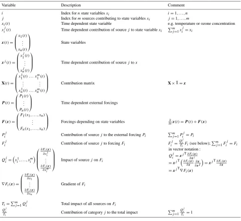
Table 1. Overview on used variables. The time dependency “(t )” is occasionally omitted for simplicity reasons, e.g.x(t )becomesx.

Variable Description Comment

i Index fornstate variablesxi i=1, . . . , n

j Index formsources contributing to state variablesxi j=1, . . . , m

xi(t ) Time dependent state variable e.g. temperature or ozone concentration

x_ij(t ) Time dependent contribution of sourcej to state variablexi Pmj=1x j i =xi

x(t )= 

 

x₁(t ) . . . xn(t )





 State variables

xj(t )= 

  

x₁j(t ) . . .

xnj(t ) 

  

Time dependent contribution of sourcej tox

X(t )= 

  

x₁1(t ) . . . x₁m(t ) .

. .

. . . x_n1(t ) . . . x_nm(t )



  

Contribution matrix XX××1==xx

P(t )= 

 

P₁(t ) . . . Pn(t )





 Time dependent external forcings

F(x)= 

 

F₁(x₁, . . . , xn) . . . Fn(x1, . . . , xn)





 Forcings depending on state variables

∂

∂tx(t )=P(t )+F(x)

P_ij Contribution of sourcejto the external forcingPi Pmj=1P j i =Pi

F_ij Contribution of sourcejto forcingFi Fij=

Qj_i

TiFi(see below);

Pm j=1F

j i =Fi

Qj_i =x1_i, . . . , x_im 

   

∂Fi(x)

∂x1

i

. . . ∂Fi(x)

∂x_im 

   

Impact of sourcejonFi

in vector notation:

Qj_i =xjT∂Fi(x)

∂xj

=xjT∂Fi(x)

∂x ∂x ∂xj

=xjT∂Fi(x)

∂x

=xjT∇Fi(x)

∇Fi(x)= 

  

∂Fi(x)

∂x₁ . . . ∂Fi(x)

∂xn



  

Gradient ofFi

Ti=Pm_j=₁Qj_i Total impact of all sources onFi

Qj_i

Ti Contribution of categoryjto the total impact

Pm j=1

Qj_i Ti =1

Obviously, the method has a singularity and hence needs special treatments for situations wherexT∇Fi(x)=0.

Be-fore this singularity will be discussed in more detail, exam-ples will be given to obtain a better understanding of the prac-tical consequences of Eq. (10) and the consistency with pre-vious tagging approaches in Grewe et al. (2010) and Grewe (2012) will be shown.

3 Examples

3.1 Self-dependency

In many cases the regarded quantity xi depends only

on a temporal forcing and on itself, i.e. F(x)=

(0, . . . ,0, f (xi),0, . . . ,0)T:

∂ ∂tx

j i =P

j

i (t )+f (xi)

x_ijf0(xi)

xif0(xi)

(11)

=P_ij(t )+f (xi)

x_ij xi

. (12)

This means that the right hand forcing term is linearly de-composed into the contributions according to the contribu-tions of the state variablex_ij.

Examples are tracers, such as Radon, which are emitted at the Earth’s surface (P_ij) and decay radioactively, i.e.f (xi)=

−xi

(4)

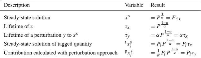
Table 2. Overview on the characteristics of the non-linear systemx˙=P−xα. See Sect. 5 for details.

Description Variable Result

Steady-state solution xs =P1α =P τx

Lifetime ofx τx =P

1−α α

Lifetime of a perturbationytoxs τy =αP 1−α

α =ατx

Steady-state solution of tagged quantity tx_is =PiP 1−α

α =Piτx

Contribution calculated with perturbation approach px_is = 1

αPiP 1−α

α =Piτy

3.2 Bimolecular reactions and similar processes

Here a reaction of two species is regarded:

x1+x2−→x3, (R1)

e.g. the reaction of NO and HO2, which forms OH and NO2

and latter photolyses and recombines to O3. Therefore, we

consider three species only, i.e.n=3. The differential equa-tion for the producequa-tion ofx3by this equation is

∂

∂tx3=F3(x)=kx1x2, (13)

withkthe reaction rate coefficient.

In this caseF3(x)=kx1x2with the notation of Eq. (10).

Withmarbitrary categories, the differential equation for the tagged speciesx₃j(j =1, . . . , m) becomes

∂ ∂tx

j

3=F3(x)

(x₁j, x₂j, x₃j)(kx2, kx1,0)T

(x1, x2, x3)(kx2, kx1,0)T

(14)

=F3(x)

kx₁jx2+kxj₂x1

2kx1x2

(15)

=F3(x)

1 2

x₁j x1

+x

j 2

x2 !

. (16)

Therefore the contribution of the categoryj to the pro-duction ofx₃j is determined by the mean contribution of the educts, i.e. 1/2(x₁j/x1+xj₂/x2). Hence it is identical to

re-sults in Grewe et al. (2010).

3.3 Ternary and multi-body reactions

Let us now consider a chemical reaction, where (m−1)

educts lead to the speciesxm:

x1+. . .+xm−1−→xm. (R2)

The differential equation for the production is then

∂

∂txm=Fm(x)=km

m−1 Y i=1

xi (17)

wherekmis the reaction rate coefficients.

The derivative of the right hand side gives

∂ ∂xi

Fm(x)=km m−1

Y k=1,k6=i

xk=

Fm(x)

xi

. (18)

And therefore, according to Eq. (10), the differential equa-tion for the contribuequa-tion results in

∂ ∂tx

j

m=Fm(x) m−1

P i=1

x_ij_∂x∂

iFm(x)

m−1 P i=1

xi_∂x∂_iFm(x)

(19)

=Fm(x) m−1

P i=1

x_ij xiFm(x)

m−1 P i=1

Fm(x)

(20)

=Fm(x)

1

m−1

m−1 X

i=1

x_ij xi

. (21)

This means that the contribution of categoryj to the pro-duction of a species xm by a (m−1)-body chemical

re-action is the mean of the contributions of the individual species (educts) xi to category j. This is again consistent

with the previously derived equations for, e.g. a ternary re-action (Grewe et al., 2010).

3.4 Heating rates

(5)

(category 1) and solar influx and shortwave absorption (cat-egory 2).

The radiation code is then called additionally twice for every “perturbation”-altitude zp with a perturbation in the

temperature and with a perturbation in the greenhouse gas concentration (in ppbv). This provides a change in the heat-ing rate profile per change in temperature and greenhouse gas concentration, respectively at all perturbation altitudes:

HT(z, zp)in s−1andHG(z, zp)in K s−1ppbv−1.

The heating profiles Hj(z) for the individual categories

j depend on both the contributions of the two categories to the temperatureTj(z)and the greenhouse gas concentration

Gj(z):

Hj(z)=H (z)

P

zp

HT(z, zp)Tj(zp)+HG(z, zp)Gj(zp)

P

zp

HT(z, zp)T (zp)+HG(z, zp)G(zp)

. (22)

Note that the magnitude in the perturbation has to be con-sidered carefully in order to avoid impacts from numerical noise, if the perturbation was chosen too small and to avoid a too large deviation from the derivative if the perturbation was chosen too large.

4 Singularities in the tagging formula

The tagging method as described in Eq. (10) has an obvi-ous disadvantage, since it may not be applicable in situation wherexT∇Fi(x) becomes zero. Fortunately, this situation

does not occur for many applications, e.g. for atmospheric chemistry or simple temperature tagging, as shown in the ex-amples in Sects. 3.1–3.3. However, some singularities remain in these examples, namely if the state variables and concen-tration of species become zero. In these cases it can be argued that since no reaction occurs, the contributions of the tagged species to the individual species remain unchanged.

In general,xT∇Fi(x)means that the sensitivities of the

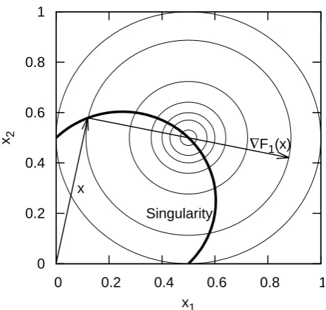
termFi are fully balanced. Figure 1 gives an example for a

two-dimensional situation, with two state variablesx1andx2.

Here, the forcing term (thin isolines) isF1(x)=0.25−(x−

a)2, withaT₌₍₁_/₂_,₁_/₂₎_{. Hence the derivative is}_∇_F 1(x)=

−2(x−a). For everyxwithxT_∇_F

1(x)=0 (thick line) the

sensitivity of the forcing termF1(x)with respect tox1, which

isx1_∂x∂

1F1(x), is balanced by the sensitivity with respect to

the second variablex2and the sum equals zero. Or in other

wordsxis perpendicular to∇F1(x)(arrows).

If we replace the forcing term byF1(x)=x1/x2 in this

example, we obtain an extreme singularity. For this forcing term the denominator in the tagging equation becomes zero:

xT∇F1(x)=(x1, x2)

1

x2

,−x1 x2₂

!T

(23)

=x1

x2

−x1

x2

=0. (24)

GMDD

5, 3311–3324, 2012

A generalized tagging method

V. Grewe

Title Page Abstract Introduction Conclusions References Tables Figures

J I

Back Close Full Screen / Esc Printer-friendly Version

Interactive Discussion

Discussion

P

a

per

|

Dis

cussion

P

a

per

|

Discussion

P

a

per

|

Discussio

n

P

a

per

|

∇F₁(x)

x

Singularity

0 0.2 0.4 0.6 0.8 1

x₁ 0

0.2 0.4 0.6 0.8 1

x2

Fig. 1.Example of a singularity in the tagging method. The forcing termF1(x) is shown in thin

lines with isolines 0.,0.1, 0.2, 0.23, 0.24, 0.245, and 0.249 with a maximum in the middle. Thick lines indicate the location of the singularitiesx∇F₁(x)=0. The arrows give an example.

3324

Fig. 1. Example of a singularity in the tagging method. The forcing termF1(x)is shown in thin lines with isolines 0., 0.1, 0.2, 0.23,

0.24, 0.245, and 0.249 with a maximum in the middle. Thick lines indicate the location of the singularitiesx∇F1(x)=0. The arrows

give an example.

Hence, for individual cases, such as atmospheric chem-istry, singularities can consistently be removed, by setting the respective forcing term to zero, with the argument that if no reaction occurs also no changes in the tagged species can oc-cur. However, as the last extreme case shows, theoretically, there are constellations, where an application of the tagging formula is not possible.

5 Comparison of diagnostical methods

As shown in the previous section, tagging is a powerful methodology to provide more insights in functional chains of non-linear systems. Evidently, many previously used di-agnostics also provided insights, however, with different as-pects. Based on a simple non-linear system, a brief inter-comparison is given here.

As a test-bed the following non-linear system is analysed:

˙

x=P−xα=:G(x), (25) whereP >0 is a production term,x >0 a state variable, and a non-linearity parameterα >0. Note that this system is lin-ear forα=1. The results are summarized in Tab. 2.

The production term has two sourcesP1>0 andP2>0

withP1+P2=P. The tagged variablesx1 andx2, which

(6)

˙

x1=P1−xα

x1

x (26)

˙

x2=P2−xα

x2

x (27)

The steady-state solutions are

xs=Pα1 ₍₂₈₎

t_xs 1=P1P

1

α−1 ₍₂₉₎

t_xs 2=P2P

1

α−1_. ₍₃₀₎

That means that the contribution of the production termP1

to the state variablexin steady-state ist_xs 1.

Using the perturbation approach, the contributionpx₁s and

p_xs

sof the source termsP1andP2to the steady-state solution

xsare calculated as

p_xs 1=

∂xs

∂P P1 (31)

= 1

αP

1

α−1_P₁ ₍₃₂₎

p_xs 2=

∂xs

∂P P2 (33)

= 1

αP

1

α−1_P₂_. ₍₃₄₎

Obviously, the solutions are equal, i.e.tx_is=px_is (i=1,2) if and only ifα=1. In general, the factor between the two approaches isα.

The decay-time or lifetime of the state variablex(and also

xi) in steady-state is

τx=

xs

xsα (35)

=P1−αα_, ₍₃₆₎

whereas any perturbation to this steady state is approximately given by the linearized perturbation equation:

˙

y= ∂

∂xG(x

s_)y ₍₃₇₎

= −αPα−1α _y. ₍₃₈₎

The Jacobian is in this case a one dimensional derivative, only. The eigenvalue analysis is simple and provides one mode, namely, the perturbation life time τy, which equals

1 αP

1−α α =τx

α and differs from the lifetime ofx by the

fac-torα. Or in other words, both life times are only equal in a linear system (α=1).

The contributions ofPi toxbased on the tagging and

per-turbation approach can then be written as

t_xs

i =Piτx (39)

p_xs

i =Piτy. (40)

In the same way, the linearized perturbation equation can be derived:

∂ ∂t

y1

y2

=

αP2+P1 P τ

−1 x τx−1

τ_x−1 αP1_P+P2τ_x−1 y1

y2

. (41) This analysis is hence a combination of an eigenvalue analy-sis, see e.g. in Prather (1998), with a tagging approach which allows for the analysis of how changes inP1andP2lead to

changes in the chemical modes of the tagged speciesx1and

x2, respectively.

6 Conclusions

In this study, a tagging approach is presented, which allows the calculation of the contribution from individual processes or quantities to state variables for application in climate-chemistry models. For these contributions, also called tagged quantities or species, differential equations are presented, which result from a partitioning of the differential equations of the primary – untagged – state variables. This partitioning is based on the sensitivity of each individual term of the right hand side forcing term with respect to the state variables.

This methodology is fully consistent with previous ap-proaches presented in Grewe et al. (2010, 2012), which were derived with a different ansatz, a combinatorial approach. Four examples show how to apply this formalism to climate-chemistry applications. One example shows how the sensitiv-ities can be derived numerically based on model internal sub-routines which were, in this case the radiation code, which provides heating rates.

An example of a very simple non-linear one-dimensional system shows how different analysis methods can be com-bined to obtain better insights. It shows that the lifetime of a species and its perturbation lifetime differ in general and co-incide if and only if the system becomes linear. In analogy, the change in the contribution of a perturbed source term to the regarded state variable (=tagged state variable) differs in general from the change in the state variable itself. Again it coincides if and only if the system becomes linear.

Despite the large possibilities, which this methodology of-fers, there are limitations to its applicability, since it may in-clude singularities. For some applications, such as for chem-ical tagging, the singularities arise from reactions, in which species are involved, which totally vanish. Since this implies that the reaction does not occur anymore, the right hand side of the tagging equation can be set to zero. This means that the involved tagged species remain unchanged, as the untagged primary species.

In a further theoretical example no consistent removal of these singularities could be found and in an extreme case the tagging formula is not applicable at all, since it consists of singularities, only.

(7)

atmospheric concentrations or temperature. The limitations show that a careful consideration of the possible singularities is necessary, when applying the tagging formula.

Acknowledgements. This work was performed during a sabbatical (DLR-Forschungssemester) at the National Center of Atmospheric Research (NCAR) in Boulder, CO and I am grateful for being given this opportunity and would like to thank all persons who made this possible. Thanks to A. Schady for internal review and helpful comments. This work was also partly funded by the EU-project REACT4C (WP2) and the DLR-internal project VEU.

Edited by: H. Tost

References

Butler, T. M., Lawrence, M. G., Taraborrelli, D., and Lelieveld, J.: Multi-day ozone production potential of volatile organic com-pounds calculated with a tagging approach, Atmos. Environ., 45, 4082–4090, 2011.

Emmons, L. K., Hess, P. G., Lamarque, J.-F., and Pfister, G. G.: Tagged ozone mechanism for MOZART-4, CAM-chem and other chemical transport models, Geosci. Model Dev., 5, 1531– 1542, doi:10.5194/gmd-5-1531-2012, 2012.

Grewe, V.: Technical Note: A diagnostic for ozone contribu-tions of various NOx emissions in multi-decadal

chemistry-climate model simulations, Atmos. Chem. Phys., 4, 729–736, doi:10.5194/acp-4-729-2004, 2004.

Grewe, V.: A new method to diagnose the contribution of anthro-pogenic activities to temperature: temperature tagging, Geosci. Model Dev. Discuss., 5, 3183–3215, doi:10.5194/gmdd-5-3183-2012, 2012.

Grewe, V., Tsati, E., and Hoor, P.: On the attribution of contributions of atmospheric trace gases to emissions in atmospheric model applications, Geosci. Model Dev., 3, 487–499, doi:10.5194/gmd-3-487-2010, 2010.

Grewe, V., Dahlmann, K., Matthes, S., and Steinbrecht, W.: At-tributing ozone to NOxemissions: implications for climate

miti-gation measures, Atmos. Environ., 59, 102–107, 2012.

Gromov, S., J¨ockel, P., Sander, R., and Brenninkmeijer, C. A. M.: A kinetic chemistry tagging technique and its application to mod-elling the stable isotopic composition of atmospheric trace gases, Geosci. Model Dev., 3, 337–364, doi:10.5194/gmd-3-337-2010, 2010.

IPCC: Climate Change 2007: The Physical Science Basis, Con-tribution of Working Group I to the Fourth Assessment Report of the Intergovernmental Panel on Climate Change, edited by: Solomon, S., Qin, D., Manning, M., Chen, Z., Marquis, M., Av-eryt, K. B., Tignor, M., and Miller, H. L., Cambridge University Press, Cambridge, UK and New York, NY, USA, 996 pp., 2007. Maas, U. and Pope, S. B.: Simplifying Chemical Kinetics: Intrinsic Low-Dimensional Manifolds in Composition Space, Combust. Flame, 88, 239–264, 1992.

Prather, M. J.: Time Scales in Atmospheric Chemistry: Coupled Perturbations to N2O, NOy, and O3, Science, 279, 1339-1441,

1998.

Uherek, E., Halenka, T., Borken-Kleefeld, J., Balkanski, Y., Berntsen, T., Borrego, C., Gauss, M., Hoor, P., Juda-Rezler, K., Lelieveld, J., Melas, D., Rypdal, K., and Schmid, S.: Transport impacts on atmosphere and climate: land transport, Atmos. Env-iron., 44, 4772–4816, 2010.