https://doi.org/10.5194/essd-9-415-2017 © Author(s) 2017. This work is distributed under the Creative Commons Attribution 3.0 License.
The MSG-SEVIRI-based cloud property
data record CLAAS-2
Nikos Benas1, Stephan Finkensieper2, Martin Stengel2, Gerd-Jan van Zadelhoff1, Timo Hanschmann2, Rainer Hollmann2, and Jan Fokke Meirink1
1Royal Netherlands Meteorological Institute (KNMI), De Bilt, the Netherlands
2Deutscher Wetterdienst (DWD), Offenbach, Germany
Correspondence to:Nikos Benas ([email protected])
Received: 8 February 2017 – Discussion started: 28 February 2017 Revised: 31 May 2017 – Accepted: 2 June 2017 – Published: 10 July 2017
Abstract. Clouds play a central role in the Earth’s atmosphere, and satellite observations are crucial for moni-toring clouds and understanding their impact on the energy budget and water cycle. Within the European Organ-isation for the Exploitation of Meteorological Satellites (EUMETSAT) Satellite Application Facility on Climate Monitoring (CM SAF), a new cloud property data record was derived from geostationary Meteosat Spinning Enhanced Visible and Infrared Imager (SEVIRI) measurements for the time frame 2004–2015. The resulting CLAAS-2 (CLoud property dAtAset using SEVIRI, Edition 2) data record is publicly available via the CM SAF website (https://doi.org/10.5676/EUM_SAF_CM/CLAAS/V002). In this paper we present an extensive evalua-tion of the CLAAS-2 cloud products, which include cloud fracevalua-tional coverage, thermodynamic phase, cloud top properties, liquid/ice cloud water path and corresponding optical thickness and particle effective radius. Data validation and comparisons were performed on both level 2 (native SEVIRI grid and repeat cycle) and level 3 (daily and monthly averages and histograms) with reference datasets derived from lidar, microwave and passive imager measurements. The evaluation results show very good overall agreement with matching spatial distribu-tions and temporal variability and small biases attributed mainly to differences in sensor characteristics, retrieval approaches, spatial and temporal samplings and viewing geometries. No major discrepancies were found. Un-derpinned by the good evaluation results, CLAAS-2 demonstrates that it is fit for the envisaged applications, such as process studies of the diurnal cycle of clouds and the evaluation of regional climate models. The data record is planned to be extended and updated in the future.
1 Introduction
Clouds are of central importance for the Earth’s energy bud-get and water cycle in modulating radiative fluxes and re-distributing water. Consistent and stable observational data records of cloud properties are needed for climate monitor-ing and evaluatmonitor-ing the distribution of clouds in weather and climate models. This requirement is reflected in the Intergov-ernmental Panel on Climate Change (IPCC)1statement that “clouds and aerosols continue to contribute the largest uncer-tainty to estimates and interpretations of the Earth’s changing energy budget” (Stocker et al., 2013, chap. 7).
1a list of abbreviations is provided in Appendix A
created within the framework of the European Organisation for the Exploitation of Meteorological Satellites (EUMET-SAT) Satellite Application Facility on Climate Monitoring (CM SAF; Schulz et al., 2009), which was recently updated (Karlsson et al., 2017).
While these datasets have global coverage, they give (apart from ISCCP) only a limited description of the temporal variability in clouds during the day. Therefore, CM SAF has been using measurements from the Spinning Enhanced Visible and Infrared Imager (SEVIRI), which is onboard the geostationary Meteosat Second Generation (MSG) satel-lites, to generate the CLoud property dAtAset using SEVIRI (CLAAS) with diurnally resolved cloud properties. The first edition of this data record (CLAAS-1) is described in Sten-gel et al. (2014). This dataset has been used to study the di-urnal cycle of clouds (e.g., Martins et al., 2016; Pfeifroth et al., 2016) and for model evaluation (e.g., Brisson et al., 2016; Alexandri et al., 2015). Recently a second reprocessed edition was released (CLAAS-2, Finkensieper et al., 2016) based on updated retrieval algorithms and incorporating mea-surements from MSG-1, 2 and 3 satellites every 15 min, thus extending the time period covered (2004–2015) and increas-ing the temporal resolution. In particular, the 15 min resolu-tion now enables process studies in which individual clouds or cloud fields need to be tracked to monitor cloud properties, such as glaciation.
In this study, the CLAAS-2 cloud properties are presented and evaluated. The data record is comprised of cloud macro-physical and micromacro-physical properties, namely cloud frac-tional coverage (CFC; derived from a corresponding cloud mask), cloud phase (CPH), which distinguishes liquid and ice clouds, cloud water path (CWP) separately for liquid (LWP) and ice (IWP) clouds and cloud top location including height (CTH), pressure (CTP) and temperature (CTT). Cloud op-tical thickness (COT) and particle effective radius (REF), which are used in the cloud water path computation, are also included. All of these properties are available as both instan-taneous data (level 2) and daily and monthly averages (level 3) along with monthly mean diurnal cycles and histograms.
The evaluation is performed by validation and intercom-parison with other cloud datasets. These include (1) observa-tions from space-based active instruments (lidar and radar), which provide the most accurate information about cloud presence in the atmosphere, (2) cloud properties derived from other passive VIS–IR satellite imagers, (3) observations of total cloud cover made at meteorological surface stations and (4) the liquid water path retrieved from spaceborne passive microwave (MW) sensors. The evaluation is performed sep-arately for level 2 and level 3 CLAAS-2 data, and their per-formance is assessed based on the different characteristics of each dataset used as a reference. Consequently, depending on the parameter being evaluated, the analysis ranges from cloud detection scores and biases to spatial distribution char-acteristics and time series comparisons.
This paper is organized as follows: in Sect. 2 the satel-lite data and algorithms used to generate the CLAAS-2 data record are described; details on the data record contents are also provided. Datasets used for the evaluation of CLAAS-2 are introduced in Sect. 3 along with the methodology used in each case. In Sect. 4 evaluation results regarding level 2 data are presented, while the corresponding results for monthly aggregated (level 3) products are described in Sect. 5. Con-cluding remarks can be found in Sect. 6.
2 The CLAAS-2 data record
2.1 SEVIRI
SEVIRI is a 12-channel imager on the MSG geostationary satellites operated by EUMETSAT. All four planned MSG satellites, Meteosat-8, 9, 10 and 11, (also referred to as MSG-1, 2, 3 and 4, respectively), have been launched. Data from the first three satellites are included in the CLAAS-2 data record covering the period from January 2004 to Decem-ber 2015. Apart from one high spatial resolution visible (HRV) channel, SEVIRI carries 11 channels between 0.6 and 14 µm with a spatial sampling resolution of 3×3 km at nadir and a 15 min repeat cycle. Further information regarding the SEVIRI channels is given in Table B1 of Appendix B. The MSG satellites have been located at similar but not exactly the same positions. Specifically, MSG-1 was positioned at 3.4◦E from 2004 to 2008. Hence, even though the SEVIRI projection in level 1.5 data is aligned at 0.0◦ for all satel-lites, the positions of the individual satellites slightly change the SEVIRI viewing geometries, which has been taken into account for the generation of the CLAAS-2 data record.
2.2 CLAAS-2
The CLAAS-2 dataset is the improved and extended follow-up to CLAAS-1 (Stengel et al., 2014). In the following, an overview of each CLAAS-2 retrieval algorithm is given, along with the main scientific updates applied, compared to the CLAAS-1 retrievals.
For the detection of clouds and their vertical place-ment, the MSGv2012 software package developed within the framework of the Nowcasting and Very Short Range Forecasting SAF (NWC SAF) was employed. Cloud detec-tion involves a series of spectral threshold tests depending on the illumination (daytime, twilight, nighttime, sun glint) and surface types among other factors. The algorithm clas-sifies satellite pixels as cloud filled, cloud free, cloud con-taminated or snow/ice concon-taminated. Further information on the cloud detection method can be found in Derrien and Le Gléau (2005), NWC SAF (2013) and Stengel et al. (2014) regarding its implementation in CLAAS-1. Compared to the MSGv2010 algorithm version, which was applied in CLAAS-1, only minor updates were implemented. These in-clude adaptations of detection tests that were affected by nocturnal extreme cooling conditions, which caused false cloud detections by the algorithm (NWC SAF, 2011), and corrections for coastal cloud mask artifacts caused by high spatial standard deviation values around coastal pixels (CM SAF, 2016a). Furthermore, contrary to the default NWC SAF MSGv2012 cloud masking algorithm, which uses 4×4 pixel segments to reduce computational time, individual thresh-olds were computed for each SEVIRI pixel in CLAAS-2. The consequent increase in the CLAAS-2 computation time was compensated for by a higher degree of parallelization.
Regarding the cloud vertical placement algorithm, no changes were implemented between the CLAAS-1 (MSGv2010) and CLAAS-2 (MSGv2012) versions. The al-gorithm, which is used for the derivation of CTH, CTP and CTT, uses input from SEVIRI channels at 6.2, 7.3, 10.8, 12.0 and 13.4 µm. The spectral information is used in the simula-tion of corresponding radiances and brightness temperatures for overcast and clear sky conditions on a pixel basis, using the Radiative Transfer for TOVS (RTTOV; Saunders et al., 1999; Matricardi et al., 2004). Ancillary data for temperature and humidity profiles from ERA-Interim are also used (Dee et al., 2011). Different approaches are used for the derivation of CTP, including a best fit between the simulated and the measured 10.8 µm brightness temperatures, the H2O–IRW (infrared window) intercept method (Schmetz et al., 1993) and the radiance rationing method (Menzel et al., 1983). Fur-ther information on the implementation of the retrieval al-gorithm for cloud top properties can be found in Stengel et al. (2014) and CM SAF (2016a).
The retrieval of CPH in CLAAS-2 was based on a modi-fied version of the Pavolonis et al. (2005) algorithm, which was provided by the Center for Satellite Applications and Re-search (STAR) of the NOAA Satellite and Information
Ser-vice (NESDIS). This approach constitutes a fundamental up-date compared to CLAAS-1, for which CPH was mainly in-ferred from CTT and the 1.6 µm reflectance. According to the new retrieval scheme, a number of spectral tests are per-formed in a specific order involving measurements from SE-VIRI channels at 6.2, 8.7, 10.8, 12.0 and 13.4 µm, as well as clear and cloudy sky IR radiances and brightness tempera-tures calculated using RTTOV. The algorithm initially yields one of the following cloud types: liquid, supercooled, opaque ice, cirrus, overlap or overshooting, which are then further condensed to liquid (former two) and ice (latter four) phase. Details on the algorithm can be found in CM SAF (2016b).
The retrieval of cloud optical and microphysical properties was based on the Cloud Physical Properties (CPP) algorithm (Roebeling et al., 2006; CM SAF, 2016b). The algorithm uses SEVIRI visible (0.6 µm) and near-infrared (1.6 µm) mea-surements to retrieve COT and REF by applying the clas-sical Nakajima and King (1990) approach. CPP is based on lookup tables (LUTs) of top-of-atmosphere (TOA) re-flectances simulated by the Doubling–Adding KNMI (DAK) radiative transfer model (Stammes, 2001), which has been frequently used in the past for numerous cloud and aerosol radiative transfer applications (e.g., de Graaf et al., 2012; Tilstra et al., 2012). The setup of these LUTs is provided in Table 1, which also contains information on the under-lying single-scattering calculations for liquid and ice cloud particles, as well as information on the assumed shape and properties of ice particles. Absorption by atmospheric trace gases is taken into account based on Moderate Resolution Atmospheric Transmission (MODTRAN4 version 2; Ander-son et al., 2001) simulations. LWP and IWP are calculated following Stephens (1978):
LWP=2
3ρlreτ, IWP= 2
3ρireτ, (1)
whereρl andρi are the densities of water and ice, respec-tively,re is REF andτ is COT. No retrievals are performed for solar zenith angles (SZAs) or viewing zenith angles (VZAs) larger than 84◦due to high uncertainties in the re-trieved properties at these angles. The main updates of CPP compared to CLAAS-1 include the generation of new LUTs with an extension in the range of SZAs and VZAs, the num-ber and range of REF and the inclusion of observational sea ice (OSI SAF, 2016) and ERA-Interim snow cover data to better characterize the surface albedo, which for all other sur-face types is taken from MODIS (Moody et al., 2005).
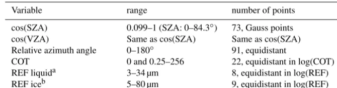
Table 1.Specification for the LUTs created with DAK. Discrete values are given for all variables spanning the axes of the LUTs.
Variable range number of points
cos(SZA) cos(VZA)
Relative azimuth angle COT
REF liquida REF iceb
0.099–1 (SZA: 0–84.3◦) Same as cos(SZA) 0–180◦
0 and 0.25–256 3–34 µm 5–80 µm
73, Gauss points Same as cos(SZA) 91, equidistant
22, equidistant in log(COT) 8, equidistant in log(REF) 9, equidistant in log(REF)
aSingle-scattering properties have been calculated using Mie theory for spherical droplets with a two-parameter gamma
size distribution (effective variance=0.15) and complex refractive index from Segelstein (1981).bSingle-scattering
properties have been calculated using ray tracing for randomly oriented monodisperse imperfect hexagonal ice crystals (Hess et al., 1998) with aspect ratios from Yang et al. (2013), roughening simulated with a distortion angle of 30◦and a complex refractive index from Warren and Brandt (2008). The choice of this ice particle model is motivated by Knap et al. (2005) who showed that it yields adequate simulations of total and polarized ice cloud reflectances observed by the Polarization and Directionality of the Earth’s Reflectances (POLDER) instrument.
threshold was only applied as a fail-safe mechanism; in prac-tice, apart from the first month of the CLAAS-2 time series (January 2004), no gaps are present in the monthly mean data. CFC was calculated from the cloud mask by count-ing cloud-free pixels as 0 and both cloud-contaminated and cloud-filled pixels as 1. In addition to the “day and night” CFC, separate averages for daytime and nighttime were com-puted. Level 3 products of cloud LWP and IWP (including COT and REF) are available during daytime only, both as cloudy-sky means and all-sky means. Apart from the regu-lar monthly aggregated products, monthly mean diurnal cy-cles have been calculated by averaging all daily mean diur-nal cycles in a month. In order to retain a sufficient num-ber of observations in each grid box, these monthly mean diurnal cycles have been prepared on a coarser spatial grid of 0.25◦×0.25◦. In addition to the mean monthly prop-erties, monthly histograms are composed by collecting the number of occurrences of cloud properties. These are CWP, CTP, CTT, COT and REF in one-dimensional, cloud-phase-separated, spatially resolved histograms with 0.05◦×0.05◦ of spatial resolution and combinations of CTP and COT in two-dimensional, cloud-phase-separated, spatially resolved histograms with 0.25◦×0.25◦of spatial resolution. The bin-ning of the histograms is given in Table 3 following Stengel et al. (2014). The REF histograms, which were not included in CLAAS-1, have bin borders of 3, 6, 9, 12, 15, 20, 25, 30, 40, 60 and 80 µm.
The CLAAS-2 data record is (as all CM SAF
climate data records) freely available online via
https://doi.org/10.5676/EUM_SAF_CM/CLAAS/V002 and includes comprehensive documentation and auxiliary data to facilitate work with the data record. CM SAF’s (www.cmsaf.eu) main task is to generate and provide climate data records (CDRs) derived from operational meteorological satellites. CDRs for components of the global energy budget and water cycle are the particular focus. During the full generation and delivery process, CM SAF adheres to the international Global Climate Observing
System (GCOS) guidelines. Thus, CM SAF applies the highest standards to make the resulting data records suitable for the analysis of climate variability and the detection of climate trends.
3 Datasets and methodology used for evaluation
In this section, the datasets used as references for the eval-uation of CLAAS-2 are described, along with the method-ology used in each case. Reference datasets are comprised of measurements from lidar, radar, microwave and passive spaceborne sensors, as well as surface observations.
3.1 CALIOP
The Cloud-Aerosol Lidar with Orthogonal Polarization (CALIOP) is a lidar instrument onboard the CALIPSO (Cloud-Aerosol Lidar and Infrared Pathfinder Satellite Ob-servation) satellite that has provided cloud and aerosol pro-file information since August 2006 (Winker et al., 2009). CALIOP products are retrieved based on backscattered sig-nal at 1064 and 532 nm and are available at horizontal and vertical resolutions of 333 and 30–60 m, respectively. They include cloud phase and type for up to 10 cloud layers per column and CTP, CTH and CTT at each layer top.
The CALIOP level 2 layered cloud products
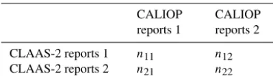
Table 2.Contingency table for the CLAAS-2 and CALIOP obser-vations;nis the number of cases and 1 and 2 correspond to clear or cloudy for the cloud mask and water or ice for the cloud phase.
CALIOP reports 1
CALIOP reports 2
CLAAS-2 reports 1 CLAAS-2 reports 2
n11 n21
n12 n22
performed using a nearest neighbor approach while tem-poral collocation was achieved by matching each CALIOP measurement time with the acquisition time of the closest SEVIRI scanline. This approach allows for maximum time and space differences of 7.5 min and 5 km, respectively.
CLAAS-2 level 2 products were validated against corre-sponding CALIOP products (Sect. 4.1). For the discrete vari-ables cloud mask (cloudy or clear) and CPH (water or ice), validation was based on statistical scores, including the prob-ability of detection (POD), the false alarm ratio (FAR), the hit rate and the Hanssen–Kuiper skill score (KSS). Downscaled spatial distributions were also compared. The formulas used for the computation of these scores are the following:
POD for event 1, 2: n11
n11+n21
, n22 n22+n12
, (2)
FAR for event 1, 2: n12
n11+n12
, n21 n22+n21
, (3)
Hit rate: n11+n22
n11+n12+n21+n22
, (4)
KSS: n11n22−n21n12
(n11+n21)(n12+n22)
. (5)
In the above formulas,nij is the number of cases for which
CLAAS-2 reports eventiand CALIOP reports eventj
(Ta-ble 2). Events correspond to cloudy and clear cases for cloud mask and water or ice clouds for CPH.
It should finally be noted that CALIOP’s higher sensitiv-ity to high and optically thin clouds, compared to SEVIRI, is an important factor affecting the validation results. In order to address this sensitivity difference and investigate the ac-curacy of CLAAS-2 products, comparisons were repeated by sampling the CALIOP profiles at successive layers below the cloud top using different thresholds for the integrated COT of these layers.
3.2 DARDAR
The DARDAR (lidar–radar) dataset was created using a synergistic approach that combines data from the Cloudsat Cloud Profiling Radar (CPR) on reflectivity, CALIOP lidar attenuated backscatter and MODIS infrared radiance mea-surements to retrieve the ice cloud properties COT, REF and IWP. The retrieval is based on an optimal estimation ap-proach, which ensures a smooth transition between regimes
for which different instruments are sensitive (Delanoë and Hogan, 2008, 2010). The products have the same vertical res-olution as CALIOP (30–60 m) and the horizontal resres-olution of CPR (700×700 m).
DARDAR data for ice COT and IWP were used for the validation of corresponding CLAAS-2 level 2 products. The DARDAR data used here are comprised of overpasses from the SEVIRI disk during January and July 2008. Extreme il-lumination geometries were excluded by selecting only re-trievals at SZAs below 75◦. Furthermore, DARDAR profiles that consist only of ice CPH were considered, and in each SEVIRI pixel a single profile was included only when all profiles in this pixel had the same CPH.
3.3 MODIS
MODIS is an advanced imaging spectroradiometer operating onboard the NASA Terra and Aqua satellites since Febru-ary 2000 and July 2002, respectively (Salomonson et al., 1989). Both the Terra and Aqua orbits are sun synchronous and timed so that they cross the equator at 10:30 and 13:30 local solar times in a descending and ascending node, respec-tively. With a viewing swath width of 2330 km, MODIS cov-ers every point on the Earth’s surface in 1 to 2 days, acquiring data in 36 spectral bands.
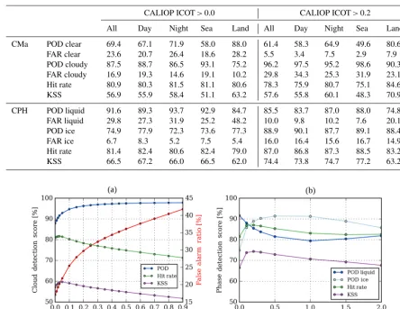
Table 3.Validation results for CLAAS-2 level 2 cloud mask (CMa) and cloud phase (CPH).
CALIOP ICOT>0.0 CALIOP ICOT>0.2
All Day Night Sea Land All Day Night Sea Land
CMa POD clear FAR clear POD cloudy FAR cloudy Hit rate KSS 69.4 23.6 87.5 16.9 80.9 56.9 67.1 20.7 88.7 19.3 80.3 55.9 71.9 26.4 86.5 14.6 81.5 58.4 58.0 18.6 93.1 19.1 81.1 51.1 88.0 28.2 75.2 10.2 80.6 63.2 61.4 5.5 96.2 29.8 78.3 57.6 58.3 3.4 97.5 34.3 75.9 55.8 64.9 7.5 95.2 25.3 80.7 60.1 49.6 2.9 98.6 31.9 75.1 48.3 80.6 7.9 90.3 23.1 84.6 70.9
CPH POD liquid FAR liquid POD ice FAR ice Hit rate KSS 91.6 29.8 74.9 6.7 81.4 66.5 89.3 27.3 77.9 8.3 82.4 67.2 93.7 31.9 72.3 5.2 80.6 66.0 92.9 25.2 73.6 7.5 82.4 66.5 84.7 48.2 77.3 5.4 79.0 62.0 85.5 10.0 88.9 16.0 87.0 74.4 83.7 9.8 90.1 16.4 86.8 73.8 87.0 10.2 87.7 15.6 87.3 74.7 88.0 7.6 89.1 16.7 88.5 77.2 74.8 20.1 88.4 14.9 83.2 63.2
Figure 1.(a)CLAAS-2 cloud detection scores as a function of the COT threshold used to discriminate clear and cloudy CALIOP observa-tions. KSS denotes the Hanssen–Kuiper skill score.(b)CLAAS-2 cloud phase detection scores as a function of the integrated COT (ICOT) threshold, which determines the reference cloud layer.
3.4 SYNOP
Total cloud cover data from surface synoptic observations (SYNOP) were used for the evaluation of CLAAS-2 level 3 monthly CFC. SYNOP data span the entire CLAAS-2 period (2004–2015) and originate from all land areas of the SEVIRI disk, with a higher density of stations in European countries. The SYNOP data used for the validation have been taken from the local DWD archive of collected global SYNOP re-ports following the guidance of the Guide to Meteorological Instruments and Methods of Observations (Jarraud, 2008). In order to ensure data quality and consistency, only SYNOP reports provided by manned airport stations were taken into account.
Monthly averaged CFC values from SYNOP stations were estimated based on corresponding daily averages. The lat-ter were calculated when at least six instantaneous measure-ments were available. Additionally, as in the CLAAS-2 level 3 case, at least 20 daily mean CFC values were required for
the estimation of monthly averages. Except for the level of agreement between the SYNOP and collocated CLAAS-2 level 3 CFC products, the dependency of this agreement on the SEVIRI VZA was also examined (Sect. 5.1).
3.5 Microwave imagers
It should be noted that, since MW measurements are not sensitive to the presence of ice clouds, the validation was limited to areas with a sufficiently low ice cloud fraction. In the SEVIRI disk this requirement is fulfilled over the marine stratocumulus (Sc) area of the southern Atlantic off the Namibian coast. Specifically, the region defined by the 20–10◦S and 0–10◦E latitude–longitude boundaries was se-lected for this purpose. Validation includes both monthly mean time series and average diurnal cycle intercomparisons of all-sky LWP computed by averaging pixel values from the Sc study region (Sect. 5.2).
4 Level 2 evaluation
In this section, the validation results of CLAAS-2 level 2 products against CALIOP and DARDAR are described. We also discuss comparisons of CLAAS-2 level 2 products with MODIS data.
4.1 Validation with CALIOP
Based on all collected CLAAS-2 level 2 and CALIOP col-locations, an overall cloud POD of 87.5 % was found, while the corresponding FAR was 16.9 % and the hit rate reached 80.9 %. Differences between day and night collocations were minor; the cloud POD was significantly higher over sea com-pared to land at the cost of an also much higher FAR.
The corresponding scores for CPH were 91.6 and 74.9 % (liquid and ice POD) and 29.8 and 6.7 % (liquid and ice FAR) with an overall CPH hit rate of 81.4 %. Both low values of ice cloud POD and high values of liquid cloud FAR should be at-tributed to CALIOP’s higher sensitivity to high and optically thin clouds. In fact, when these clouds are excluded from the analysis, ice cloud scores acquire higher values with ice POD becoming similar to the liquid POD, while liquid cloud FAR is reduced to 10.0 % when the CALIOP phase was sampled at a COT of 0.2 below the cloud top. These results are sum-marized in Table 3.
This difference in sensitivity between CLAAS-2 and CALIOP was further analyzed using a varying CALIOP to-tal column COT as a threshold for distinguishing cloud-free from cloudy scenes. Hence, all CALIOP scenes with a COT of less than this threshold were set as cloud free. Results are shown in Fig. 1a with the COT threshold on the x axis. It is clear that as the COT threshold used to distinguish clear and cloudy CALIOP measurements increases, both POD and FAR increase. The POD increases because optically thin clouds, which are likely not to be detected by SEVIRI, are also excluded from CALIOP and the number of scenes in which both CALIOP and CLAAS-2 detect clouds increases. However, as the COT threshold increases, some clouds that are detected by SEVIRI are also excluded from CALIOP; such cases cause an increase in FAR. These combined effects cause the hit rate and KSS to peak at COT≈0.05.
The effect of using the CALIOP CPH for the layer at which the integrated COT (ICOT) exceeds a certain thresh-old instead of the uppermost layer is shown in Fig. 1b. Ap-plying this ICOT threshold leads to an increase in ice cloud POD, since thin ice clouds detected by CALIOP but not by SEVIRI are excluded. There are two ways the liquid POD can be influenced when excluding a thin CALIOP ice cloud and instead comparing against a liquid CALIOP cloud lo-cated below. If the thin ice cloud was incorrectly reported as liquid by CLAAS-2, the liquid POD would increase; it would decrease if the cloud was correctly reported as ice by CLAAS-2. It was found that occurrences of the second case increased with ICOT 3 times more than the first, leading to the decrease in liquid cloud POD shown in Fig. 1b.
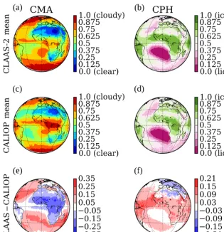
Figure 2 shows the spatial distributions of the cloud frac-tion and the ice cloud fracfrac-tion estimated from all collocated CLAAS-2 level 2 and CALIOP measurements. The maps were created by remapping matchups to a regular 1.5◦×1.5◦ grid and averaging within each grid box. Large-scale patterns between the two datasets are similar for both the cloud frac-tion and phase. There is a tendency for CLAAS-2 to over-estimate cloud fraction over the northern and southern At-lantic as well as the Indian Ocean, which may be related to the high VZAs over these areas (Reuter et al., 2009). On the other hand, the cloud fraction in the tropics is underes-timated by CLAAS-2, probably due to the frequent presence of cirrus clouds in this area, which are more likely to be de-tected by CALIOP (Sun et al., 2011). The phase agreement is very good overall, with slightly fewer ice clouds reported by CLAAS-2 over Africa and the central Atlantic, which is consistent with the difference in the cloud fraction over the same areas.
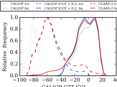
Taking the CALIOP CTT as a reference, the relation of CTT and CPH was also examined (Fig. 3). The agreement is excellent in both liquid and ice cloud histograms when using
ICOT=0.2 as a threshold layer for CALIOP CTT and CPH
selection. It should be noted that the CLAAS-2 histogram ex-tensions above 0◦C for ice clouds (red dashed line in Fig. 3) and below−42◦C for liquid clouds (red solid line in Fig. 3) should be attributed to the fact that thex axis CTT binning in this figure comes from CALIOP. The CLAAS-2 CTT is always below 0◦C for ice clouds and above−42◦C for liq-uid clouds. Hence, these histogram extensions are related to CALIOP retrieving higher CTT (former case) or lower CTT (latter case) than CLAAS-2. If CLAAS-2 CTT was used in-stead, such cases would not be allowed by the retrieval algo-rithm.
Figure 2.Spatial distribution of the cloud fraction from CLAAS-2 level 2(a)and CALIOP(c)and the fraction of ice clouds (bandd). The bottom row shows the absolute difference in CLAAS and CALIOP for the cloud fraction(e)and the fraction of ice clouds(f). Note the different scaling in(e)and(f). The CALIOP cloud detection criterion is total column COT>0, while the CALIOP phase is taken from the layer at which ICOT exceeds 0.2.
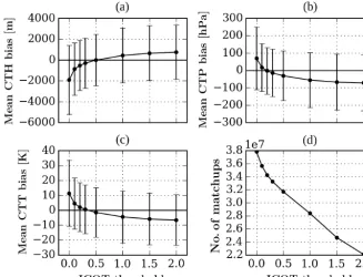
top layers based on different ICOT threshold values, a strong influence was found (Fig. 4). All biases acquire their min-imum absolute values at an ICOT threshold of about 0.3– 0.5 and their signs are reversed as the ICOT of CALIOP ex-cluded cloud top layers increased towards 2.0. The spread of CLAAS-2 compared to CALIOP data is also reduced, as can be seen from the bias-corrected root mean square error (bc-RMSE) represented as error bars in Fig. 4.
In contrast to level 2 cloud mask and cloud phase ables, which acquire values of only 0 or 1, cloud top vari-ables are continuous so that a correlation analysis can be performed. The results are shown as scatterplots in Fig. 5. The overall correlation is strong in all cloud top products, with Pearson correlation coefficients ranging between 0.84 and 0.88. The least-squares fit slopes are below 1, which also reflects the underestimation in CTH and overestimation in CTP and CTT of high clouds by CLAAS-2.
4.2 Validation with DARDAR
Figure 6a shows the CLAAS-2 versus DARDAR ice COT comparison. The distribution contours show the number of points enclosed, e.g., the black area (central contour) en-closes the 20 % of bins containing the largest density of observations. The distribution is clearly correlated and lies along the 1:1 line. However, the remaining 25 % of the ob-servations outside of the density contours (not shown in the figure) are so scattered that the total correlation remains weak (0.33).
Figure 3.Phase histograms for liquid and ice clouds as a function of CALIOP cloud top temperature. For the red and blue lines, bin-ning is based on the CALIOP CTT taken from the layer at which ICOT exceeds 0.2. For the light blue line, the phase and tempera-ture of the uppermost CALIOP cloud layer were used. Bin size is 4◦C.
These results highlight the difficulty in interpreting an evaluation of passive versus active instruments. The main reasons for this difficulty include the different microphysical assumptions applied in the retrievals and the difference be-tween column-averaged (but weighted to the top of the cloud) retrievals from variable viewing geometries for the passive instrument versus profile information from a near-nadir view for the active instruments.
4.3 Comparison with MODIS
For the level 2 CLAAS-2 comparison with MODIS Collec-tion 6, one Terra MODIS granule is shown as a case study. The granule on 20 June 2008 from 10:50 to 10:55 UTC, covering the largest part of Europe, was selected because it fulfilled a number of criteria, including a balanced pres-ence between low and high, liquid and ice and thin and thick clouds, as well as relatively low SZAs. The time difference between the two datasets was also minimized by selecting the 10:45 UTC SEVIRI time slot, which covered Europe at around 10:56 UTC.
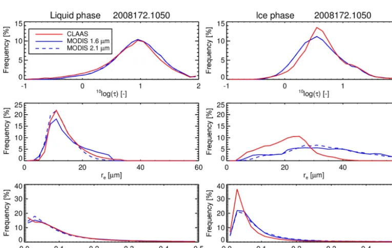
Figure 7 shows histograms of CLAAS-2 and MODIS COT, REF and CWP from this granule separately for liq-uid and ice clouds, created using only collocations for which CPH was the same in both datasets. The liquid COT his-tograms reveal good agreement, while ice COT is slightly larger in CLAAS-2 than in MODIS. Relative peaks at
COT=100 should be attributed to the fact that COT
re-trievals greater than 100 are set equal to 100, causing the relatively higher number of pixels found with this value. The MODIS 1.6 and 2.1 µm REF retrievals yield slightly differ-ent histograms. Considering that the CLAAS-2 products are
based on 1.6 µm measurements, it is somewhat surprising that the CLAAS-2 REF agrees better with the MODIS 2.1 µm product than the 1.6 µm, especially in the liquid cloud case. For ice clouds, CLAAS-2 acquires an overall lower REF, which is most probably related to the choice of ice particle habits; i.e., the severely roughened monodisperse hexagonal columns for CLAAS-2 versus the severely roughened aggre-gated columns with a gamma size distribution (Yang et al., 2013) for MODIS C6. Consistent with the results of the REF intercomparison, the agreement for LWP is better than for IWP.
5 Level 3 evaluation
This section covers the evaluation of CLAAS-2 level-3 prod-ucts for daily and monthly aggregations and monthly mean diurnal cycles.
5.1 Validation with SYNOP
The comparison of CLAAS-2 monthly mean CFC data with corresponding SYNOP observations showed overall good agreement with a CLAAS-2-SYNOP bias (over all SYNOP stations) of 3.7 % on average and a 7.5 % maximum. This bias, however, is positive for the entire time series as a con-sequence of the well-known effect of cloudiness overestima-tion by passive satellite sensors at high VZAs (e.g., Maddux et al., 2010) in combination with most SYNOP stations be-ing located in central Europe, away from the SEVIRI nadir viewpoint.
This effect was verified by a more detailed analysis of the dependency of CFC bias on VZA. The results of this anal-ysis are shown in Fig. 8, for which CFC bias values have
been averaged in 10◦ VZA bins along with the bc-RMSE
values, which gives a measure of the precision of CLAAS-2 observations, and the number of observations available from
SYNOP. The bias is negative for VZAs below 40◦and
Figure 4.Mean biases (CLAAS-2–CALIOP) of CTH(a), CTP(b)and CTT(c)compared against the CALIOP cloud layer at which ICOT exceeds a certain threshold. The error bars represent the bc-RMSE. The number of collocated measurements is also shown(d).
Figure 5.Scatterplots of cloud top products between CLAAS-2 and CALIOP: CTH(a), CTP(b)and CTT(c). The diagonal is marked by a solid line, and the dashed lines show the result of a least-squares linear fit. The text box in the upper left corner displays the Pearson correlation coefficient. Thepvalues are practically zero because of the very large number of matchups. CALIOP values were taken from the layer at which ICOT exceeds 0.2 in all plots.
5.2 Validation with UWisc
Figure 9a shows the time series plot of the monthly all-sky LWP at 12:00 UTC from CLAAS-2 and UWisc, calculated over the marine Sc region west of Namibia (0–10◦E, 10– 20◦S). The two data records exhibit similar seasonal char-acteristics, with the largest differences appearing almost ev-ery year in August and September when CLAAS-2 acquires lower values compared to the UWisc all-sky LWP. This char-acteristic should be attributed to the presence of absorbing aerosols over the clouds, originating from biomass burning activities during this season; these overlying aerosols cause a negative bias in the LWP retrieval (Haywood et al., 2004).
Figure 6.(a)Ice COT distribution comparing the collocated values retrieved from DARDAR and CLAAS-2. The blue dashed line is the 1:1 line and the gray scales indicate the regions enclosing 20, 40, 60 and 75 % of all data points.(b)As in(a)for the IWP. The yellow line depicts the median and the orange lines represent the 16th and 84th percentiles of the CLAAS-2 distribution at the corresponding DARDAR IWP.(c)1-D histogram of DARDAR and CLAAS-2 IWP for the same collocations.
Figure 7. Histograms of CLAAS-2 and MODIS COT (top), REF (middle) and CWP (bottom) for the selected MODIS granule on 20 June 2008. The left panels are liquid clouds and the right panels are ice clouds. Only pixels for which both products agree on CPH are included. For MODIS the standard and PCL (partly cloudy) retrievals were combined, and results are shown for retrievals with two different wavelength bands (1.6 and 2.1 µm). Note that differences between MODIS 1.6 and 2.1 µm based on COT are small. Hence, the solid and dashed blue lines in the top panels cannot be distinguished.
increase that may be a retrieval artifact related to illumination geometry (high SZAs).
5.3 Comparison with MODIS
Figure 10 shows the intercomparison of CLAAS-2 and MODIS level 3 spatial distributions computed by averaging monthly data from the entire CLAAS-2 period, along with their differences. In the CFC and CPH cases (Fig. 10a and c), MODIS data are based on the cloud mask product, which is affected by the Terra calibration drift issue. Hence, an
in-tercomparison only with Aqua MODIS data was performed in these two cases, as described in Sect. 3.3.
Figure 8.Dependency of the level 3 CLAAS-2–SYNOP CFC bias, bc-RMSE and SYNOP number of observations on the SEVIRI viewing zenith angle.
Figure 9.(a)Time series of the monthly all-sky LWP over the marine Sc region (0–10◦E, 10–20◦S) at 12:00 UTC from CLAAS-2 and UWisc data.(b)Monthly mean diurnal cycle of all-sky LWP from CLAAS-2 and UWisc over the same region.
opposite sign over land and ocean that is most pronounced e.g., over South America, Europe and the Red Sea. Fig-ure 10b shows the CTH distributions and differences. Over-all, CLAAS-2 tends to estimate higher cloud top heights, with the exceptions of central Africa and the Sahara where for the latter region CFC is minimal. The southern Atlantic marine Sc clouds are also placed slightly lower in CLAAS-2. The fraction of liquid clouds, expressed in CPH, is shown in Fig. 10c. As expected, the patterns are similar to the CTH case, with liquid clouds clearly prevailing at lower CTHs. Compared to MODIS, CLAAS-2 retrieves more ice clouds at the eastern and western edges of the disk and more liquid clouds around the 60◦S zone. Figure 10d shows the spatial distribution of the all-sky LWP from CLAAS-2 and MODIS
Figure 11. Time series of the 45◦W–E and S–N area-averaged CFC(a), CTH(b), CPH (liquid cloud fraction)(c), all-sky LWP(d)
and all-sky IWP(e)from CLAAS-2 and MODIS. Aqua MODIS data were used in(a)and(c); average Aqua and Terra MODIS data were used in(b),(d)and(e).
The lower CLAAS-2 IWP is consistent with the level-2 com-parisons in Fig. 7, demonstrating that it is mainly explained by differences in the effective radius retrievals.
Overall, the intercomparison of temporally averaged dis-tributions shows that CLAAS-2 and MODIS are in good agreement. In all the variables shown in Fig. 10, additional possible reasons causing differences between the datasets in-clude the diurnal variability in clouds, which is not fully cap-tured by MODIS, differences in cloud masking algorithms and the spatial averaging processes being used for the pro-duction of level 3 data.
Figure 11 shows the time series of the area-weighted av-erages of CLAAS-2 and MODIS level 3 cloud products over the 45◦W–E and S–N region. This area was selected instead of the entire SEVIRI disk to ensure consistency in the time series of the daytime products in all seasons.
6 Data availability
The CM SAF CLAAS-2 data record is freely available at https://doi.org/10.5676/EUM_SAF_CM/CLAAS/V002. The site provides documentation, related publications and links to auxiliary data, further data record details and ordering.
7 Summary
This study focused on the validation and intercomparison of the recently released cloud property data record CLAAS-2 by CM SAF based on measurements from the SEVIRI sen-sor onboard the geostationary satellites MSG-1, 2 and 3. The main characteristics of the retrieval algorithms used for the creation of CLAAS-2 were described, along with their up-dates compared to the first CLAAS edition.
A variety of reference datasets from different sensors and based on different retrieval approaches were used to evalu-ate and intercompare the CLAAS-2 retrievals at all possible processing levels. Validation was based on active sensors, which are considered the most accurate measurements of cloud properties in the atmosphere, and on ground-based ob-servations. Intercomparisons were made with MODIS, which is one of the most advanced passive sensors with retrievals similar to those used in CLAAS-2.
The results revealed overall good agreement between CLAAS-2 and the reference datasets. While no major dis-crepancies were found, the differences reported can be at-tributed to various factors ranging from different retrieval ap-proaches (e.g., profile retrievals from active sensors versus column-integrated retrievals from passive sensors), different microphysical assumptions in otherwise similar methodolo-gies (e.g., between CLAAS-2 and MODIS) and differences in spatial and temporal samplings and viewing geometries. Considering all these factors, the results presented here con-firm the reliability and stability of CLAAS-2 data.
In view of the present findings, CLAAS-2 can be con-sidered a valuable source of data for studies on clouds and their role in the (regional) climate system. By making use of the advantages of a geostationary imager, it combines high spatial and temporal resolutions, rendering the data prod-ucts suitable for both local- and continental-scale studies at time frames ranging from sub-hourly processes to interan-nual variability.
Appendix A: List of abbreviations
AMSR-E Advanced Microwave Scanning Radiometer for Earth Observing System
AVHRR Advanced Very High-Resolution Radiometer
bc-RMSE Bias-corrected root mean square error
CALIOP Cloud-Aerosol Lidar with Orthogonal Polarization
CALIPSO Cloud-Aerosol Lidar and Infrared Pathfinder Satellite Observation
CDR Climate data record
CFC Cloud fractional coverage
CLAAS Cloud property dAtAset using SEVIRI
CLARA CM SAF cLoud, Albedo and surface RAdiation dataset
CM SAF Satellite Application Facility on Climate Monitoring
COT Cloud optical thickness
CPH Cloud phase
CPP Cloud Physical Properties
CPR Cloud Profiling Radar
CTH Cloud top height
CTP Cloud top pressure
CTT Cloud top temperature
CWP Cloud water path
DAK Doubling–Adding KNMI
DARDAR raDAR–liDAR
ERA-Interim ECMWF Reanalysis Interim Dataset
ECMWF European Centre for Medium-Range Weather Forecasts
EUMETSAT European Organisation for the Exploitation of Meteorological Satellites
FAR False alarm ratio
GCOS Global Climate Observing System
HRV High Spatial Resolution Visible Channel
ICOT Integrated COT
IPCC Intergovernmental Panel on Climate Change
IR Infrared
ISCCP International Satellite Cloud Climatology Project
ITCZ Intertropical Convergence Zone
IWP Ice water path
KSS Hanssen–Kuiper skill score
LUT Lookup table
LWP Liquid water path
MODIS Moderate Resolution Imaging Spectroradiometer
MODTRAN Moderate Resolution Atmospheric Transmission
MSG Meteosat Second Generation
MW Microwave
NASA National Aeronautics and Space Administration
NESDIS NOAA Satellite and Information Service
NOAA National Oceanic and Atmospheric Administration
NWC SAF Nowcasting and Very Short Range Forecasting Satellite Application Facility OSI SAF Ocean and Sea Ice Satellite Application Facility
PATMOS-x Pathfinder Atmospheres-Extended
POD Probability of detection
REF Effective radius
RTTOV Radiative Transfer for TOVS
SEVIRI Spinning Enhanced Visible and Infrared Imager
SSM/I Special Sensor Microwave Imager
STAR Center for Satellite Applications and Research
SYNOP Surface synoptic observations
SZA Solar zenith angle
TOA Top-of-atmosphere
TOVS TIROS Operational Vertical Sounder
TRMM Tropical Rainfall Measuring Mission
UWisc University of Wisconsin
VIS Visible
Appendix B: Spectral characteristics of SEVIRI channels
Table B1.MSG SEVIRI channels. Specifications include channel number, central wavelength (µm) and nominal spectral bandwidth (µm).
Channel Central wavelength Spectral bandwidth
HRV 1 2 3 4 5 6 7 8 9 10 11
n/a 0.635 0.81 1.64 3.92 6.25 7.35 8.70 9.66 10.80 12.00 13.40
About 0.4–1.1 0.56–0.71 0.74–0.88 1.50–1.78 3.48–4.36 5.35–7.15 6.85–7.85 8.30–9.10 9.38–9.94 9.80–11.80 11.00–13.00 12.40–14.40
Competing interests. The authors declare that they have no con-flict of interest.
Acknowledgements. The authors thank Andrew Heidinger (NOAA) for the provision of the modified version of the Pavolo-nis et al. (2005) cloud phase algorithm.
This work was performed within CM SAF funded by EUMET-SAT in cooperation with the national meteorological services of Germany, Sweden, Finland, the Netherlands, Belgium, Switzerland and the United Kingdom.
Edited by: Alexander Kokhanovsky Reviewed by: two anonymous referees
References
Alexandri, G., Georgoulias, A. K., Zanis, P., Katragkou, E., Tsik-erdekis, A., Kourtidis, K., and Meleti, C.: On the ability of RegCM4 regional climate model to simulate surface solar ra-diation patterns over Europe: an assessment using satellite-based observations, Atmos. Chem. Phys., 15, 13195–13216, https://doi.org/10.5194/acp-15-13195-2015, 2015.
Anderson, G. P., Berk, A., Acharya, P. K., Matthew, M. W., Bern-stein, L. S., Chetwynd, J. H., Dothe, H., Adler-Golder, S. M., Ratkowski, A. J., Felde, G. W., Gardner, J. A., Hoke, M. L., Richtsmeier, S. C., and Jeong, L. S.: MODTRAN4 version 2: radiative transfer modeling, P. SPIE, 4381, 455–459, 2001. Baum, B. A., Menzel, W. P., Frey, R. A., Tobin, D. C., Holz, R.
E., Ackerman, S. A., Heidinger, A. K., and Yang, P.: MODIS Cloud-Top Property Refinements for Collection 6, J. Appl. Me-teorol. Clim., 51, 1145–1163, https://doi.org/10.1175/JAMC-D-11-0203.1, 2012.
Brisson, E., Van Weverberg, K., Demuzere, M., Devis, A., Saeed, S., Stengel, M., and Van Lipzig, N. P. M.: How well can a convection-permitting climate model reproduce decadal statis-tics of precipitation, temperature and cloud characterisstatis-tics?, Clim. Dynam., 47, 3043–3061, https://doi.org/10.1007/s00382-016-3012-z, 2016.
CM SAF: Algorithm Theoretical Basis Document, SE-VIRI cloud products, CLAAS Edition 2, EUMET-SAT Satellite Application Facility on Climate Monitor-ing, SAF/CM/DWD/ATBD/SEV/CLD, Issue 2, Rev. 3, https://doi.org/10.5676/EUM_SAF_CM/CLAAS/V002, 17 June 2016a.
CM SAF: Algorithm Theoretical Basis Document, SEVIRI Cloud Physical Products, CLAAS Edition 2, EUMET-SAT Satellite Application Facility on Climate Monitor-ing, SAF/CM/KNMI/ATBD/SEVIRI/CPP, Issue 2, Rev. 2, https://doi.org/10.5676/EUM_SAF_CM/CLAAS/V002, 10 June 2016b.
de Graaf, M., Tilstra, L. G., Wang, P., and Stammes, P.: Re-trieval of the aerosol direct radiative effect over clouds from spaceborne spectrometry, J. Geophys. Res., 117, D07207, https://doi.org/10.1029/2011JD017160, 2012.
Dee, D. P., Uppala, S. M., Simmons, A. J., Berrisford, P., Poli, P., Kobayashi, S., Andrae, U., Balmaseda, M. A., Balsamo, G., Bauer, P., Bechtold, P., Beljaars, A. C. M., van de Berg, L.,
Bid-lot, J., Bormann, N., Delsol, C., Dragani, R., Fuentes, M., Geer, A. J., Haimberger, L., Healy, S. B., Hersbach, H., Hólm, E. V., Isaksen, L., Kallberg, P., Köhler, M., Matricardi, M., McNally, A. P., Monge-Sanz, B. M., Morcrette, J.-J., Park, B.-K., Peubey, C., de Rosnay, P., Tavolato, C., Thépaut, J.-N., and Vitart, F.: The ERA-Interim reanalysis: configuration and performance of the data assimilation system, Q. J. Roy. Meteor. Soc., 137, 553–597, 2011.
Delanoë, J. and Hogan, R. J.: A variational scheme for re-trieving ice cloud properties from combined radar, lidar, and infrared radiometer, J. Geophys. Res., 113, D07204, https://doi.org/10.1029/2007JD009000, 2008.
Delanoë, J. and Hogan, R. J.: Combined CloudSat-CALIPSO-MODIS retrievals of the properties of ice clouds, J. Geophys. Res., 115, D00H29, https://doi.org/10.1029/2009JD012346, 2010.
Derrien, M. and Le Gléau, H.: MSG/SEVIRI cloud mask and type from SAFNWC, Int. J. Remote Sens., 26, 4707–4732, 2005. Eliasson, S., Holl, G., Buehler, S. A., Kuhn, T.,
Sten-gel, M., Iturbide-Sanchez, F., and Johnston, M.: System-atic and random errors between collocated satellite ice water path observations, J. Geophys. Res.-Atmos., 118, 2629–2642, https://doi.org/10.1029/2012JD018381, 2013.
Finkensieper, S., Meirink, J. F., van Zadelhoff, G.-J., Han-schmann, T., Benas, N., Stengel, M., Fuchs, P., Holl-mann, R., and Werscheck, M.: CLAAS-2: CM SAF CLoud property dAtAset using SEVIRI – Edition 2. Satellite Application Facility on Climate Monitoring, https://doi.org/10.5676/EUM_SAF_CM/CLAAS/V002, 2016. Haywood, J. M., Osborne, S. R., and Abel, S. J.: The effect of
over-lying absorbing aerosol layers on remote sensing retrievals of cloud effective radius and cloud optical depth, Q. J. Roy. Meteor. Soc., 130, 779–800, 2004.
Heidinger, A. K., Foster, M. J., Walther, A., and Zhao, X.: The Pathfinder Atmospheres Extended (PATMOS-x) AVHRR climate data set, B. Am. Meteorol. Soc., 95, https://doi.org/10.1175/BAMS-D-12-00246.1, 2014.
Hess, M., Koelemeijer, R. B. A., and Stammes, P.: Scattering matri-ces of imperfect hexagonal ice crystals, J. Quant. Spectrosc. Ra., 60, 301–308, 1998.
Jarraud, M.: Guide to Meteorological Instruments and Methods of Observation (WMO – No. 8), World Meteorological Organisa-tion, Geneva, Switzerland, 2008.
Karlsson, K.-G.: A ten-year cloud climatology over Scandinavia de-rived from NOAA AVHRR imagery, Int. J. Climatol., 23, 1023– 1044, https://doi.org/10.1002/joc.916, 2003.
Karlsson, K.-G., Riihelä, A., Müller, R., Meirink, J. F., Sedlar, J., Stengel, M., Lockhoff, M., Trentmann, J., Kaspar, F., Holl-mann, R., and Wolters, E.: CLARA-A1: a cloud, albedo, and radiation dataset from 28 yr of global AVHRR data, Atmos. Chem. Phys., 13, 5351–5367, https://doi.org/10.5194/acp-13-5351-2013, 2013.
global AVHRR data, Atmos. Chem. Phys., 17, 5809–5828, https://doi.org/10.5194/acp-17-5809-2017, 2017.
Knap, W. H., Labonnote, L. C., Brogniez, G., and Stammes, P.: Modeling total and polarized reflectances of ice clouds: evalu-ation by means of POLDER and ATSR-2 measurements, Appl. Optics, 44, 4060–4073, 2005.
Maddux, B. C., Ackerman, S. A., and Platnick, S.: Viewing Geometry Dependencies in MODIS Cloud Products, J. Atmos. Ocean. Tech., 27, 1519–1528, https://doi.org/10.1175/2010JTECHA1432.1, 2010.
Martins, J. P. A., Cardoso, R. M., Soares, P. M. M., Trigo, I. F., Belo-Pereira, M., Moreira, N., and Tomé, R.: The summer diurnal cycle of coastal cloudiness over west Iberia using Meteosat/SEVIRI and a WRF regional cli-mate model simulation, Int. J. Climatol., 36, 1755–1772, https://doi.org/10.1002/joc.4457, 2016.
Matricardi, M., Chevallier, F., Kelly, G., and Thepaut, J.-N.: An im-proved general fast radiative transfer model for the assimilation of radiance observations, Q. J. Roy. Meteor. Soc., 130, 153–173, https://doi.org/10.1256/qj.02.181, 2004.
Meirink, J. F., Roebeling, R. A., and Stammes, P.: Inter-calibration of polar imager solar channels using SEVIRI, Atmos. Meas. Tech., 6, 2495–2508, https://doi.org/10.5194/amt-6-2495-2013, 2013.
Menzel, W. P., Smith, W. L., and Stewart, T. R.: Improved Cloud Motion Wind Vector and Altitude Assignment using VAS, J. Appl. Meteorol. Clim., 22, 377–384, 1983.
Moody, E. G., King, M. D., Platnick, S., Schaaf, C. B., and Gao, F.: Spatially complete global spectral surface albedos: value-added datasets derived from Terra MODIS land products, IEEE T. Geosci. Remote S., 43, 144–158, 2005.
Nakajima, T. and King, M. D.: Determination of the optical thick-ness and effective particle radius of clouds from reflected solar radiation measurements, part 1: Theory, J. Atmos. Sci., 47, 1878– 1893, 1990.
NWC SAF: Scientific report on improving “Cloud Products” (CMa-PGE01 v3.1, CT-PGE02 v2.1 & CTTH-PGE03 v2.2), EUMET-SAT Satellite Application Facility on Nowcasting and Short range Forecasting, SAF/NWC/CDOP/MFL/SCI/RP/06, Issue 1, Rev. 0, 24 March 2011.
NWC SAF: Algorithm Theoretical Basis Document for “Cloud Products” (CMa-PGE01 v3.2, CT-PGE02 v2.2 and CTTH-PGE03 v2.2), EUMETSAT Satellite Applica-tion Facility on Nowcasting and Short range Forecasting, SAF/NWC/CDOP2/MFL/SCI/ATBD/01, Issue 3, Rev. 2.1, 15 July 2013.
O’Dell, C. W., Wentz, F. J., and Bennartz, R.: Cloud liquid water path from satellite-based passive microwave observations: a new climatology over the global oceans, J. Climate, 21, 1721–1739, 2008.
OSI SAF: The EUMETSAT OSI SAF Sea Ice Concen-tration Algorithm. Algorithm Theoretical Basis Document, SAF/OSI/CDOP/DMI/SCI/MA/189, Version 1.5, 2016. Pavolonis, M. J., Heidinger, A. K., and Uttal, T.: Daytime global
cloud typing from AVHRR and VIIRS: Algorithm description, validation, and comparison, J. Appl. Meteorol., 44, 804–826, https://doi.org/10.1175/JAM2236.1, 2005.
Pfeifroth, U., Trentmann, J., Fink, A., and Ahrens, B.: Eval-uating Satellite-Based Diurnal Cycles of Precipitation in
the African Tropics, J. Appl. Meteorol. Clim., 55, 23–39, https://doi.org/10.1175/JAMC-D-15-0065.1, 2016.
Platnick, S., King, M. D., Meyer, K. G., Wind, G., Amaras-inghe, N., Marchant, B., Arnold, G. T., Zhang, Z., Hubanks, P. A., Ridgway, B., and Riédi, J.: MODIS Cloud Opti-cal Properties: User Guide for the Collection 6 Level-2 MOD06/MYD06 Product and Associated Level-3 Datasets, Ver-sion 1.0, available at http://modis-atmos.gsfc.nasa.gov/_docs/ C6MOD06OPUserGuide.pdf (last access: 31 May 2016), 2015. Platnick, S. E., King, M. D., Ackerman, S. A., Menzel, W. P., Baum,
B. A., Riédi, J. C., and Frey, R. A.: The MODIS cloud products: Algorithms and examples from Terra, IEEE T. Geosci. Remote S., 41, 459–473, 2003.
Reuter, M., Thomas,W., Albert, P., Lockhoff, M.,Weber, R., Karls-son, K.-G., and Fischer, J.: The CM-SAF and FUB Cloud Detec-tion Schemes for SEVIRI: ValidaDetec-tion with Synoptic Data and Ini-tial Comparison with MODIS and CALIPSO, J. Appl. Meteorol. Clim., 48, 301–316, https://doi.org/10.1175/2008JAMC1982.1, 2009.
Roebeling, R. A., Feijt, A. J., and Stammes, P.: Cloud property retrievals for climate monitoring: implications of differences between SEVIRI on METEOSAT-8 and AVHRR on NOAA-17, J. Geophys. Res., 111, D20210, https://doi.org/10.1029/2005JD006990, 2006.
Rossow, W. B. and Schiffer, R. A.: Advances in understanding clouds from ISCCP, B. Am. Meteorol. Soc., 80, 2261–2287, 1999.
Salomonson, V. V., Barnes, W. L., Maymon, P. W., Montgomery, H. E., and Ostrow, H.: MODIS: Advanced facility instrument for studies of the earth as a system, IEEE T. Geosci. Remote S., 27, 145–153, https://doi.org/10.1109/36.20292, 1989.
Saunders, R., Matricardi, M., and Brunel, P.: An improved fast radiative transfer model for assimilation of satellite radi-ance observations, Q. J. Roy. Meteor. Soc., 125, 1407–1425, https://doi.org/10.1002/qj.1999.49712555615, 1999.
Schmetz, J., Holmlund, K., Hoffman, J., Strauss, B., Mason, B., Gaertner, V., Koch, A., and Van De Berg, L.: Operational cloud motion winds from Meteosat infrared images, J. Appl. Meteorol., 32, 1206–1225, 1993.
Schulz, J., Albert, P., Behr, H.-D., Caprion, D., Deneke, H., Dewitte, S., Dürr, B., Fuchs, P., Gratzki, A., Hechler, P., Hollmann, R., Johnston, S., Karlsson, K.-G., Manninen, T., Müller, R., Reuter, M., Riihelä, A., Roebeling, R., Selbach, N., Tetzlaff, A., Thomas, W., Werscheck, M., Wolters, E., and Zelenka, A.: Operational cli-mate monitoring from space: the EUMETSAT Satellite Applica-tion Facility on Climate Monitoring (CM-SAF), Atmos. Chem. Phys., 9, 1687–1709, https://doi.org/10.5194/acp-9-1687-2009, 2009.
Segelstein, D.: The complex refractive index of water, MSc Thesis, University of Missouri, Kansas City, 1981.
Stammes, P.: Spectral radiance modelling in the UV-Visible range, in: IRS 2000: Current problems in Atmospheric Radiation, edited by: Smith, W. L. and Timofeyev, Y. M. A., Deepak, Hampton, VA, 385–388, 2001.
Stephens, G.: Radiation profiles in extended water clouds, II: Pa-rameterization schemes, J. Atmos. Sci., 35, 2123–2132, 1978. Stocker, T. F., Qin, D., Plattner, G.-K., Tignor, M., Allen, S. K.,
Boschung, J., Nauels, A., Xia, Y., Bex, V., and Midgley, P. (Eds.): Climate Change 2013: The physical science basis. Contribution of Working Group I to the Fifth Assessment Report of the Inter-governmental Panel on Climate Change, Cambridge University Press, Cambridge, United Kingdom and New York, NY, USA, 2013.
Sun, W., Videen, G., Kato, S., Lin, B., Lukashin, C., and Hu, Y.: A study of subvisual clouds and their radiation effect with a synergy of CERES, MODIS, CALIPSO and AIRS data, J. Geophy. Res., 116, D22207, https://doi.org/10.1029/2011JD016422, 2011. Tilstra, L. G., de Graaf, M., Aben, I., and Stammes, P.:
In-flight degradation correction of SCIAMACHY UV reflectances and Absorbing Aerosol Index, J. Geophys. Res., 117, D06209, https://doi.org/10.1029/2011JD016957, 2012.
Warren, S. G. and Brandt, R. E.: Optical constants of ice from the ultraviolet to the microwave: A revised compilation, J. Geophys. Res., 113, D14220, https://doi.org/10.1029/2007JD009744, 2008.
Winker, D. M., Vaughan, M. A., Omar, A., Hu, Y., Pow-ell, K. A., Liu, Z., Hunt, W. H., and Young, S. A.: Overview of the CALIPSO Mission and CALIOP data pro-cessing algorithms, J. Atmos. Ocean. Tech., 26, 2310–2323, https://doi.org/10.1175/2009JTECHA1281.1, 2009.
Wu, A., Xiong, X., Doelling, D. R., Morstad, D., Angal, A., and Bhatt, R.: Characterization of Terra and Aqua MODIS VIS, NIR, and SWIR spectral bands’ calibration stability, IEEE T. Geosci. Remote S., 51, 4330–4338, 2013.