https://doi.org/10.5194/gmd-10-4577-2017 © Author(s) 2017. This work is distributed under the Creative Commons Attribution 4.0 License.
The SPACE 1.0 model: a Landlab component for 2-D calculation
of sediment transport, bedrock erosion, and landscape evolution
Charles M. Shobe, Gregory E. Tucker, and Katherine R. Barnhart
CIRES and Department of Geological Sciences, University of Colorado, Boulder, Colorado, USA Correspondence:Charles M. Shobe ([email protected])
Received: 15 July 2017 – Discussion started: 4 August 2017
Revised: 10 November 2017 – Accepted: 11 November 2017 – Published: 18 December 2017
Abstract. Models of landscape evolution by river erosion are often either transport-limited (sediment is always avail-able but may or may not be transportavail-able) or detachment-limited (sediment must be detached from the bed but is then always transportable). While several models incorpo-rate elements of, or transition between, transport-limited and detachment-limited behavior, most require that either sedi-ment or bedrock, but not both, are eroded at any given time. Modeling landscape evolution over large spatial and tem-poral scales requires a model that can (1) transition freely between transport-limited and detachment-limited behavior, (2) simultaneously treat sediment transport and bedrock ero-sion, and (3) run in 2-D over large grids and be coupled with other surface process models. We present SPACE (stream power with alluvium conservation and entrainment) 1.0, a new model for simultaneous evolution of an alluvium layer and a bedrock bed based on conservation of sediment mass both on the bed and in the water column. The model treats sediment transport and bedrock erosion simultaneously, em-bracing the reality that many rivers (even those commonly defined as “bedrock” rivers) flow over a partially alluvi-ated bed. SPACE improves on previous models of bedrock– alluvial rivers by explicitly calculating sediment erosion and deposition rather than relying on a flux-divergence (Exner) approach. The SPACE model is a component of the Land-lab modeling toolkit, a Python-language library used to cre-ate models of Earth surface processes. Landlab allows effi-cient coupling between the SPACE model and components simulating basin hydrology, hillslope evolution, weathering, lithospheric flexure, and other surface processes. Here, we first derive the governing equations of the SPACE model from existing sediment transport and bedrock erosion formu-lations and explore the behavior of local analytical solutions
for sediment flux and alluvium thickness. We derive steady-state analytical solutions for channel slope, alluvium thick-ness, and sediment flux, and show that SPACE matches pre-dicted behavior in detachment-limited, transport-limited, and mixed conditions. We provide an example of landscape evo-lution modeling in which SPACE is coupled with hillslope diffusion, and demonstrate that SPACE provides an effective framework for simultaneously modeling 2-D sediment trans-port and bedrock erosion.
1 Introduction
diver-gence of sediment transport capacity (e.g., Paola and Voller, 2005). Detachment-limited models (e.g., Howard, 1994) as-sume that erosion is limited by a river’s ability to remove sediment or rock from the bed but that all detached mate-rial is transportable. As such, they include no statement of mass conservation (aside from the assumption that all eroded mass leaves the model domain) because all detached mass is assumed to be transported downstream. Transport capacity in transport-limited models and detachment rate in detachment-limited models are generally assumed to be some function of water quantity and slope (e.g., shear stress or stream power). In this paper, we briefly discuss the problem of differ-entiating between these two end-member models and how previous workers have attempted model validation in the field. We review existing models that fall between the two end-members and argue that many models are limited by an inability to treat simultaneous sediment transport and bedrock erosion over landscape evolution timescales. We then describe the SPACE (stream power with alluvium con-servation and entrainment) 1.0 model, a new channel evo-lution model intended to simulate the long-term evoevo-lution of bedrock–alluvial channels at the landscape scale. SPACE calculates sediment transport and bedrock erosion simulta-neously by modeling the coupled evolution of an alluvial layer and a bedrock bed. We show that the SPACE model transitions smoothly between transport-limited, detachment-limited, and mixed behavior, and that it matches analytical solutions for channel slope, sediment layer thickness, and sediment flux. We use the example of topographic evolu-tion in response to unsteady rock uplift to show that as a component of the Landlab toolkit, SPACE may be coupled with other landscape evolution model components to explore landscape change over long timescales. Finally, we discuss the potential for field validation of the SPACE model, the limitations of the model, and the similarities and differences between SPACE and previous channel evolution models.
2 The problem of model differentiation and applicability
While the underlying assumptions of the transport-limited and detachment-limited end-member models differ, they pro-duce identical steady-state longitudinal profiles (e.g., Whip-ple and Tucker, 2002; Lague et al., 2003). Further, as noted by Davy and Lague (2009), the applicability of one end-member model or the other to a given landscape appears to depend on the characteristics of test sites and on the com-parison methods (e.g., Snyder et al., 2003a; Tomkin et al., 2003; van der Beek and Bishop, 2003; Valla et al., 2010; Hobley et al., 2011). Such tests generally consist of using models to match topographic variables such as erosion rate– channel steepness scaling (e.g., Snyder et al., 2003a), match-ing steady-state model solutions to river profiles with evi-dence for steady-state behavior (e.g., Tomkin et al., 2003),
using a well-constrained initial condition and present-day to-pography to compare river profile evolution between mod-els and the landscape (e.g., van der Beek and Bishop, 2003; Valla et al., 2010), or combining fluvial erosion depths with field model calibration to find an optimal model form (e.g., Hobley et al., 2011). Both end-member models have been shown to be applicable in certain landscapes. For example, both Valla et al. (2010) and Hobley et al. (2011) investi-gated the carving of postglacial gorges (in the Alps and the Himalaya, respectively) and both used gorge incision depth and other field measurements to validate transport-limited and detachment-limited incision models. Valla et al. (2010) concluded that a transport-limited model was most appropri-ate for treating gorge incision at their study site, while Hob-ley et al. (2011) found that gorge evolution in the Himalaya was best replicated with a detachment-limited model. Nei-ther the detachment-limited nor the transport-limited end-member model has been shown to agree with field data in a wide variety of natural settings, likely due in large part to the potential for both types of behavior to occur simultaneously. This suggests that to apply to real landscapes, landscape evo-lution models must include both sediment mass conservation (as in transport-limited models) and sediment production/bed erosion (as in detachment-limited models). Below, we re-view some of these models, specifically focusing on those that treat both sediment transport and bedrock erosion.
3 Review of sediment transport and bedrock erosion models
Over the past two decades, new efforts to advance model-ing of bedrock–alluvial river channel evolution have focused on (1) improving descriptions of sediment mass conserva-tion and transport, and (2) improving formulaconserva-tions for bed erosion. Additionally, several models have been developed that combine statements of mass conservation and bed ero-sion in order to simulate simultaneous sediment transport and bed evolution. We focus specifically on those models combining sediment dynamics and erosion into bedrock, as our goal is the development of a model for the evolution of mixed bedrock–alluvial channels. Substantial advances have also been made in modeling the hydrodynamics that drive channel evolution, but we do not review that work here. 3.1 Approaches to mass conservation
deposition approach, in which erosion and deposition fluxes of sediment are calculated to determine changes in sediment flux and alluvial layer thickness. Either type of mass con-servation statement may be used to model bedrock–alluvial rivers. Inoue et al. (2014) used a modified 1-D Exner equa-tion for sediment mass conservaequa-tion incorporating both mo-bile bed load and an alluvial layer. Lague (2010) and Zhang et al. (2015) followed a similar approach, further modify-ing the sediment mass conservation framework to include below-capacity sediment transport. Exner sediment transport in bedrock–alluvial systems was expanded to 2-D by Nelson and Seminara (2012) and Inoue et al. (2016, 2017), though the specifics of calculating sediment flux differ between the model of Nelson and Seminara (2012) and the latter two. The Exner-based conservation framework allows calculation of bed cover by sediment as a function of the ratio of sediment flux to transport capacity (qs/qc) (Inoue et al., 2014). Inoue
et al. (2014) predicted a range of cover functions depend-ing on the ratio of grain roughness to bedrock roughness, ranging from an exponential decline in exposed bed frac-tion with increasingqs/qcto rapid alluviation above aqs/qc
threshold. Other models for alluvial bed cover arise from simplifications to the Exner-style approach. Johnson (2014) made steady-state predictions for alluvial cover as a func-tion ofqs/qcon a non-erodible bedrock bed, and showed that
bedrock roughness relative to sediment size is an important control on setting the influence ofqs/qcon bed cover. Nelson
and Seminara (2011) assumed that sediment was transported at capacity at every point along a 2-D channel cross section in order to compute the thickness of alluvial cover in the cross section.
The erosion–deposition framework differs from the Exner approach in that it conserves mass on the bed and in the wa-ter column to treat simultaneous erosion and deposition of a single substrate (Beaumont et al., 1992; Braun and Sam-bridge, 1997; Coulthard et al., 2002; Davy and Lague, 2009; Carretier et al., 2016). Erosion–deposition mass conserva-tion is based on explicit calculaconserva-tions of sediment entrain-ment and deposition, rather than on the spatial divergence of sediment transport capacity. Erosion–deposition models may dynamically transition between transport-limited and detachment-limited behavior (see discussion by Davy and Lague, 2009). Davy and Lague (2009) present such a model based on the relative influence of erosion from the bed into the water column (erosion flux) and deposition from the wa-ter column onto the bed (deposition flux). When the depo-sition flux is much smaller than the erosion flux, and the sediment transport length scale, which can be thought of as the average travel distance of a grain from entrainment to redeposition, is long, their model becomes equivalent to a basic detachment-limited model. When the deposition flux increases and the transport length scale is short, the model predicts transport-limited behavior in which sediment flux divergence controls the channel bed elevation. The erosion– deposition framework, validated for alluvial rivers by the
lab-oratory experiments of Lajeunesse et al. (2017), is capable of matching transient and steady-state longitudinal profile predictions made by both detachment-limited and transport-limited models, and smoothly transitions between the two types of model behavior (Davy and Lague, 2009). The model of Davy and Lague (2009) improved on previous erosion– deposition models (Beaumont et al., 1992) by using a sed-iment transport length scale that increases with water dis-charge. Erosion–deposition-type models that transition be-tween detachment-limited and transport-limited behavior al-low the exploration of both types of models, and intermediate cases, with simple parameter changes rather than changes to the model structure.
Erosion–deposition models, like Exner-based transport models, can yield predictions for the influence of sediment dynamics on erosion-inhibiting sediment bed cover. The models of Hodge and Hoey (2012), Nelson and Seminara (2012), and Turowski and Hodge (2017) incorporate state-ments of sediment mass conservation to explore cover dy-namics on a stationary bedrock bed. Hodge and Hoey (2012) used a cellular automaton model of alluvial cover evolution that allowed probabilistic entrainment and deposition of sed-iment on a non-eroding bedrock bed. They found that either a linear or exponential decline in bedrock exposure with in-creasingqs/qccould occur if all grains had equal entrainment
probability, with the exponential decline occurring at low en-trainment probabilities and the linear decline occurring at high entrainment probabilities. Additionally, they found that when isolated grains have a higher entrainment probability than clustered grains, bedrock exposure declines sigmoidally with increasing qs/qc and runaway alluviation can occur.
Their results support the experimental results of Chatanan-tavet and Parker (2008) showing that both the linear decline in exposure with increasingqs/qcand the abrupt shift from
fully exposed to fully alluviated bed are possible, with the former occurring at low slopes and high bed roughness, and the latter occurring at high slopes and low bed roughness. Turowski and Hodge (2017) explicitly tracked erosion and deposition governing the transfer of particles between two mass reservoirs: the stationary particles on a non-erodible bedrock bed and the mobile particles in the water column. They showed that the relationship between bedrock expo-sure andqs/qccan take a wide range of forms depending on,
among other factors, the probability of increasing bed cover for a given fraction of exposed bed.
3.2 Approaches to bedrock erosion
dis-charge) and channel bed slope. The major limitation of basic stream power and shear stress models is the lack of a de-scription of how sediment influences channel bed erosion. A large number of sediment-flux-dependent incision mod-els, in which the interaction of sediment flux with sediment transport capacity enhances or inhibits bedrock erosion, have been developed to fill this gap (e.g., Sklar and Dietrich, 1998, 2004; Whipple and Tucker, 2002; Gasparini et al., 2006, 2007; Turowski et al., 2007; Chatanantavet and Parker, 2009; Hobley et al., 2011). Sediment may act as “cover,” inhibiting bedrock erosion, or as “tools,” accelerating bedrock erosion (see review by Hobley et al., 2011). In most sediment-flux-dependent models, erosion is influenced by a factorf (qs, qc)
ranging between 0 and 1, where qs is sediment flux (either
volume or mass flux per unit width) andqcis sediment
trans-port capacity. The value off (qs, qc)for any particularqsand
qcdepends on the choice of functionf; proposed forms
in-clude a linear decline (f (qs, qc)=1−qqcs; Beaumont et al.,
1992), parabola (Sklar and Dietrich, 2004), near-parabola (Gasparini et al., 2006), and other similar shapes (Turowski et al., 2007). Turowski et al. (2007) showed that the frac-tion of exposed bed may decline exponentially with increas-ingqs/qc, leading to an exponential tail onf (qs, qc). Any of
the formulations for bedrock erosion detailed here are insuf-ficient on their own for modeling bedrock–alluvial channels, as there is no mass conservation of sediment and therefore no development of an alluvial layer. Any bedrock erosion model may be coupled with a statement of mass conservation to capture the coupled evolution of bedrock–alluvial channels. 3.3 Coupled sediment transport and bedrock erosion
models
While several existing erosion–deposition models contain descriptions of both sediment mass conservation and bed erosion, some are limited to erosion through a single sub-strate, and are not capable of evolving a bedrock-alluvial channel with a distinct alluvial layer (e.g., Davy and Lague, 2009; Carretier et al., 2016). Carretier et al. (2016) presented a model in which the erosion–deposition framework is ap-plied to cases in which a layer of sediment overlies bedrock, but their model requires that one or the other material fully occupy the surface of a cell at a given time. Without sub-stantial modification, erosion–deposition models are there-fore unable to simultaneously treat sediment morphodynam-ics and bedrock erosion in mixed bedrock–alluvial systems. A small subset of existing channel evolution models combine sediment mass conservation with equations for bedrock inci-sion to treat bedrock–alluvial channels. For example, Lague (2010) used the Exner equation for sediment conservation to explicitly track a layer of alluvium of thicknessTswith
me-dian grain sizeD50overlying a bedrock bed. He tested both
the linear and the exponential forms of the decline in bed exposure with increasing qs/qc, both expressed as a
func-tion of the ratio of Ts to D50 (his Fig. 3). The model of
changes in sediment supply. Their model tracks the thick-ness of a sediment layer compared to the macro-roughthick-ness of the bedrock surface such that alluvial thickness less than the macro-roughness length scale results in exposed bedrock. Their geometric approach is similar to that of Lague (2010), but the Zhang et al. (2015) model incorporates both tools and cover effects due to its derivation from the saltation–abrasion model (Sklar and Dietrich, 2004). While Zhang et al. (2015) note that their model could incorporate downstream varia-tions in channel width, it does not do so in the form they presented.
3.4 Reach-scale vs. landscape-scale approaches
The models reviewed above differ in their intended spatial and temporal scales of application. For example, the cross-section saltation–abrasion model of Nelson and Seminara (2011) resolves flow hydraulics and channel width varia-tions with high fidelity but cannot be feasibly applied at the landscape scale. Similarly, the bed cover evolution models of Turowski (2009), Hodge and Hoey (2012), Nelson and Seminara (2012), Johnson (2014), and Turowski and Hodge (2017) focus specifically on cover dynamics at the reach scale. While principles from these models could be incor-porated into larger-scale landscape evolution models, several of the models (Hodge and Hoey, 2012; Nelson and Semi-nara, 2012; Johnson, 2014; Turowski and Hodge, 2017) are formulated for a fixed bedrock bed, thus limiting their poten-tial for application to problems of long-term landscape evo-lution. The 2-D mixed bedrock–alluvial models proposed by Inoue et al. (2016, 2017) could potentially be incorporated into existing landscape evolution model frameworks, but the feasibility of such an integration is unclear as the models have been tested over hourly to daily timescales, not geo-logic timescales. The models most suited to landscape evo-lution applications are those of Fowler et al. (2007), Lague (2010), Inoue et al. (2014), and Zhang et al. (2015). The In-oue et al. (2014) model realistically incorporates hydraulic roughness of both bedrock and alluvium but is designed to handle a constant sediment supply rate, a constraint which is unlikely to be satisfied in landscape evolution modeling ap-plications. The model of Fowler et al. (2007) assumes no sup-ply limitation on sediment flux and is thus not suited to mod-eling mixed bedrock–alluvial cases. The two existing models that most closely match our goal of treating bedrock–alluvial channel dynamics over landscape evolution space scales and timescales are those of Lague (2010) and Zhang et al. (2015). We advance on these models by using the erosion–deposition sediment conservation framework to craft explicit expres-sions for the entrainment and deposition of sediment as well as the erosion of bedrock.
3.5 The SPACE model
We present a new model for simultaneous sediment and bedrock evolution that extends from the approaches of Davy and Lague (2009), Lague (2010), and Zhang et al. (2015), as well as from the foundation laid by the other models re-viewed above. The SPACE model conserves sediment in two reservoirs, the bed and the water column, in the style of Davy and Lague (2009). It is therefore an erosion–deposition model in its treatment of sediment. SPACE also calculates bedrock erosion, incorporating progressive bedrock exposure with thinning of an alluvial layer in a similar way to Lague (2010) and Zhang et al. (2015) such that evolution of the al-luvium and the bedrock may be simultaneously calculated. SPACE is unique in that it employs local analytical solutions for sediment flux changes in space and alluvium thickness changes in time. These local analytical solutions are derived by combining expressions for conservation of sediment in the water column (e.g., Davy and Lague, 2009), conservation of sediment on the channel bed, and conservation of mass of bedrock. Our new model advances beyond sediment-flux-dependent bedrock incision models in which sediment trans-port and storage are not treated explicitly, as well as previous erosion–deposition models assumed to be eroding a single substrate. The SPACE model is designed to run over large spatial and temporal scales in two dimensions, and can be easily coupled to many other surface process models as part of the Landlab modeling toolkit.
The SPACE model is intended to model river channel evo-lution over long timescales while honoring the reality that channels may transition between alluviated, bedrock, and mixed bedrock–alluvial states over geologic time. Below, we develop the SPACE model, verify our numerical solutions against analytical solutions, and show that SPACE can tran-sition naturally between transport-limited and detachment-limited behavior. We briefly describe the Landlab modeling toolkit and show an example landscape evolution model in which SPACE is coupled to other surface process models.
4 SPACE model development
The SPACE model, like other erosion–deposition models, arises from sediment mass conservation in the water column (e.g., Davy and Lague, 2009) and on the channel bed. We consider a river bed that may vary dynamically in its rela-tive proportion of alluvial cover and exposed bedrock, with a bedrock surface of heightR, bed sediment of mean thickness H (the channel bed elevationηis thereforeR+H), and wa-ter of mean flow depthh(Fig. 1). We use the term “SPACE model” to refer to the model equations, and “SPACE 1.0 component” to refer specifically to the numerical implemen-tation of the SPACE model as a Landlab component. 4.1 Conservation of sediment in the water column Davy and Lague (2009) showed that the rate of change in the volume of sediment in the water column per unit area of river bed ∂(csh)
∂t may be written as
∂ (csh)
∂t =Es−Ds−
∂ (Qs/w)
∂x , (1)
wherecs is the concentration of sediment in the water
col-umn calculated byQs/Q(whereQis volumetric water
dis-charge), Es is the volumetric entrainment flux of sediment
per unit bed area, Ds is the volumetric deposition flux of
sediment per unit bed area, Qs is sediment flux in units of
[L3/T], andw is channel width. Equation (1) is sufficient when considering a channel bed on which only a single ma-terial (i.e., sediment) is exposed. Yet many channels are par-tially alluviated, indicating that sediment and bedrock may be eroded and entrained into the water column simultane-ously. Such a scenario requires an addition to Eq. (1) to ac-count for entrainment of bedrock material into the water col-umn:
∂ (csh)
∂t =Es+(1−Ff) Er−Ds−
∂ (Qs/w)
∂x . (2)
Er is the volumetric erosion flux of bedrock per unit bed
area.Ffis a unitless fraction of fine sediment.Ffrepresents
the volumetric fraction of bedrock that breaks into sediment small enough to be considered permanently in suspension, for which no further treatment of bed–water column interac-tions is needed. For bedrock that breaks only into sand and
gravel fractions,Ffwould be zero. Therefore, bed sediment
thickness H and sediment flux Qs only include sediment
coarse enough that it does not enter permanent suspension. Assuming that ∂(csh)
∂t =0 (an important model assumption
that potentially restricts applicability to hydrograph-scale modeling), the spatial gradient in sediment flux is a balance between sediment entrainment, rock erosion, and sediment deposition:
∂ (Qs/w)
∂x =Es+(1−Ff) Er−Ds. (3) 4.2 Conservation of sediment and rock on the channel
bed
Change of channel bed elevation with time is the sum of changes in rock height and sediment thickness:
∂η ∂t =
∂R ∂t +
∂H
∂t . (4)
Following Eq. (4) and Davy and Lague (2009), conservation of sediment on the channel bed with sediment thicknessH may be written as
∂H ∂t =
Ds−Es
1−φ , (5)
whereφis the porosity of the bed sediment. Because there is no deposition of bedrock, the rate of change of bedrock elevationRover time is
∂R
∂t =U−Er, (6)
whereU is the rock uplift rate relative to base level. For simplicity, we assume that the porosity of rock is zero, but rock porosity could easily be added to Eq. (6). Steady sedi-ment thickness requires equal erosion and deposition of sed-iment(Ds=Es)and steady bedrock elevation requires that
erosion of rock is balanced by rock uplift relative to base level(U=Er). Figure 1 shows a schematic of a model cell
and defines relevant variables.
4.3 Entrainment of bed sediment and erosion of bedrock
As discussed by Davy and Lague (2009), any number of ac-cepted expressions for entrainment of bed sediment and ero-sion of bedrock could be used forEsandEr, respectively. We
R
H Q
dx
dx Qsin
Qs
Es
Ds Qs
Er
U
Figure 1.Conceptual sketch of a single model cell and definition of variables. Rock surface elevationRis defined as the elevation of the lowest point on the bedrock surface and is also used as the lower boundary for the thicknessHof the alluvial layer.
stream power but is also influenced by sediment thickness H relative to a reach-scale bedrock roughness length scale H∗. At lowH /H∗, the lower points on the bedrock bed are
mantled with sediment, but high points on the bedrock sur-face are still exposed. At high H /H∗, all areas of the bed
are covered with sediment. Further, Es must be zero when
H is zero and no sediment is available to be entrained, and Es must reach a maximum (for a given stream power) when
there is enough sediment to fully cover the bed (Fig. 2). This approach is conceptually similar to the models of Tur-owski et al. (2007), Lague (2010) (his exponential model), and Zhang et al. (2015), and similarly eliminates the need to explicitly track bedrock exposure. Given the conceptual model described above, the entrainment rate of sedimentEs
may be written as Es= KsqSn−ωcs
1−e−H /H∗, (7)
whereKsis the sediment erodibility parameter,Sis
channel-bed slope, andnis a scaling exponent.q is water discharge per unit channel width and may be calculated by any number of methods. The simplest isq=kqAm, whereAis drainage
area,mis a scaling exponent (generally ≈0.5) designed to reflect downstream width changes and discharge–area scal-ing (Leopold and Maddock, 1953; Snyder et al., 2003b; Wohl and David, 2008), andkqis an empirical constant, with units
dependent on the value of m, that is subsumed into Ks and
the rock erodibility parameterKr. Using the volumetric
wa-ter flux per unit channel widthq results inKs andKr
hav-ing dimensions of
L−1
.ωcs is a threshold stream power
required for sediment entrainment. In very simple cases,ωcs
may be neglected, but the ability to include a threshold term is important in any river evolution model as threshold effects have been shown to significantly alter model outcomes (Sny-der et al., 2003a; Tucker, 2004; Lague et al., 2005; DiBi-ase and Whipple, 2011). While we employ a simple
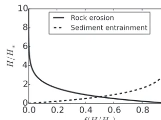
clo-Figure 2. Dimensionless efficiency of erosion and deposition (f (H /H∗)) for different values ofH /H∗. Erosive power is
mul-tiplied byf (H /H∗)in the model to account for the relative
ex-posure of sediment and bedrock. Such a formulation accounts for the fact that bedrock beds are rough, and low points may become sediment mantled while high points remain exposed (e.g., John-son, 2014; Zhang et al., 2015).H∗is therefore a length scale
repre-senting reach-scale bedrock roughness. Sediment entrainment for a given stream power increases with increasingH /H∗, while bedrock
erosion declines as a response to sediment mantling of the bed. At values ofH /H∗≈6, all bed lowering is driven by sediment
entrain-ment and bedrock erosion is negligible. This heuristic representa-tion of mixed bedrock–alluvial channel dynamics is conceptually similar to the approaches taken by Lague (2010) and Zhang et al. (2015).
sure for channel width in which width scales as the square root of water discharge (e.g., Leopold and Maddock, 1953; Wohl and David, 2008), it may be desirable for some ap-plications to add dynamic channel width adjustments to the model, as previous work has suggested that width trades off with slope in transient channels (e.g., Finnegan et al., 2005; Turowski et al., 2006; Wobus et al., 2006; Whittaker et al., 2007; Attal et al., 2008; Lague, 2010; Yanites and Tucker, 2010). One option for incorporating dynamic width is to cal-culate or approximate shear–stress distributions across chan-nel cross sections (e.g., Kean and Smith, 2004; Wobus et al., 2006, 2008; Turowski et al., 2009). A simpler dynamic width rule can be obtained by partitioning erosive power between the bed and banks under a trapezoidal channel assumption (Flintham and Carling, 1988) as detailed by Lague (2010). Different approaches have different numbers of parameters and computational costs, and further work will be necessary to elucidate which advances beyond the standard empirical width closure are tractable within the SPACE landscape evo-lution model framework.
2007; Hobley et al., 2011), the volumetric erosion rate of bedrock per unit bed area may be written as
Er= KrqSn−ωcre−H /H∗. (8)
Here, Kr is the bedrock erodibility parameter, which is
generally expected to be substantially lower than Ks. ωcr
is the threshold stream power for detachment of bedrock, which may vary significantly depending on the relative dom-inance of plucking or abrasion (e.g., Hancock et al., 1998; Whipple et al., 2000) as well as the weathered state of the bedrock (Hancock et al., 2011; Johnson and Finnegan, 2015; Small et al., 2015; Murphy et al., 2016; Shobe et al., 2017). Howard (1998), Hancock and Anderson (2002), Turowski et al. (2007), and Lague (2010) employed a similar expo-nential decline in rock erosion rate with increasing sediment thickness. Equation (8) falls into the category of “cover” models, which treat erosion reduction by sediment shield-ing the bed without incorporatshield-ing the potential erosive ef-fects of mobile sediment (e.g., Beaumont et al., 1992; Lague, 2010; Shobe et al., 2016). The smooth transitions between bare-bedrock, bedrock–alluvial, and fully alluviated chan-nels given by Eqs. (7) and (8) are both more stable and more realistic than models in which the existence of any alluvium fully covers the bedrock (implying a perfectly smooth, pla-nar bedrock surface). Figure 2 shows the pattern of sedi-ment entrainsedi-ment and bedrock erosion over different values ofH /H∗.f (H /H∗)in Fig. 2 is the dimensionless exposure
term that modifies stream power entrainment and erosion in Eqs. (7) and (8) (i.e.,e−H /H∗or(1−e−H /H∗)). Perhaps the most significant simplification in our model is that we do not include explicit treatment of the erosive effects of grains in transport (e.g., Sklar and Dietrich, 1998, 2001, 2004; Gas-parini et al., 2006; Turowski et al., 2007; Lamb et al., 2008; Cook et al., 2013). Such an effect could enhance sediment entrainment if grains in saltation hit resting grains and en-abled their entrainment, and could enhance bedrock ero-sion if sediment-rich water were flowing over well-exposed bedrock. The “tools effect” on bedrock erosion could be in-corporated into the model by assuming that Er at a given
H /H∗ increases withQs until Qs reaches transport
capac-ity (which isQswhenEs+Er=Ds). Because increases in
H /H∗already account for the “cover effect,” theEr
depen-dence on Qs need only be positive and not decline with
in-creasingQs(e.g., Sklar and Dietrich, 2001; Gasparini et al.,
2006; Turowski et al., 2007). We assume for the purposes of model validation against analytical solutions that these ef-fects are negligible relative to changes in unit stream power and bed cover.
The major advantages of the exponential entrainment and erosion approach outlined here are that (1) sedi-ment and bedrock may be simultaneously entrained/eroded into the water column, (2) the presence of sediment does not completely inhibit bedrock erosion at low values of H /H∗, which is supported by modeling and observations
of mixed bedrock–alluvial channels (Johnson et al., 2009;
Johnson, 2014; Ferguson et al., 2017; Hodge, 2017), and (3) model stability is improved because sediment thick-ness gradually approaches zero, preventing a sudden transi-tion from sediment entrainment to bedrock erosion. Many different rules for sediment entrainment and bedrock ero-sion could be used in this model framework in place of stream-power-type equations. No matter how erosive power is calculated, the SPACE approach allows both erodibil-ity and entrainment/detachment thresholds to be chosen independently for sediment and bedrock, unlike in strict detachment-limited/transport-limited models or the basic form of erosion–deposition models. This enables the treat-ment of systems with multiple erosion thresholds, such as a river for which bedrock erosion requires both mobilization of an alluvial cover (described byωcs) and the plucking of
bedrock blocks (described byωcr).
power becomes larger than the defined threshold, entrain-ment and erosion should increase smoothly as a greater por-tion of the distribupor-tion of thresholds is exceeded. In the limit where available stream power is many times greater than the user-defined threshold, available stream power should sim-ply be reduced by the user-defined threshold. An exponential function describing the increase in entrainment/erosion as available stream power increases relative to threshold stream power satisfies these requirements without adding any model parameters. We include an optional exponential expression for threshold stream power such that entrainment/erosion does not go immediately to zero when stream powerωequals the threshold value ωc but declines exponentially as ω/ωc
declines. The threshold stream power is expected to be dif-ferent for rock than for sediment, withωcrlikely being larger
in most cases than ωcs. In this formulation, the expressions
for sediment entrainment and bedrock erosion (Eqs. 7 and 8) become
Es= KsqSn−ωcs 1−e−ω/ωcs
1−e−H /H∗ (9) and
Er= KrqSn−ωcr 1−e−ω/ωcre−H /H∗. (10)
Inspection of Eqs. (9) and (10) reveals that whenωωc, the
threshold term approachesωc, yielding behavior identical to
single-value threshold models. When ω=ωc, the threshold
represents approximately 63 % (1−e−1) of available stream power, rather than 100 % as in the basic threshold approach. Whenωωc, the threshold term approachesωand the
en-trainment or erosion rate approaches zero. We chose an expo-nential function because it allows for smoothing of entrain-ment and erosion thresholds, and therefore honors the reality that such thresholds tend to be distributions of values rather than a single value, without adding any model parameters. Evaluation of the full behavior of models using an exponen-tially declining threshold is beyond the scope of this paper, and the use of Eqs. (9) and (10) is optional in the SPACE model.
4.4 Deposition of sediment
The flux of sediment from the water column onto the bed is the product of sediment concentration averaged over the depth of the water column and effective sediment settling ve-locityV (Davy and Lague, 2009):
Ds=csV =
Qs
QV . (11)
V is not the still-water particle settling velocity but is the net effective settling velocity after accounting for the upward effects of turbulence. V also incorporates the vertical gra-dient in sediment concentration through the water column (d∗in Davy and Lague, 2009). In an equivalent formulation, Davy and Lague (2009) treated the sediment deposition rate
asDs=d∗csV, whered∗is a dimensionless number that
re-lates sediment concentration near the bed to mean sediment concentration in the water column. Equation (11) assumes that sediment and water move at the same speed such that all changes in Qs
Q are driven by erosion and deposition.
4.5 Steady-state analytical solutions
We develop steady-state analytical solutions for sediment flux Qs, channel slope S, and bed sediment thickness H,
all of which are steady when ∂(csh)
∂t =0. We assume for the
purposes of this derivation that there are no entrainment or erosion thresholds, and thatFf andφ are both negligible –
assumptions that are easily relaxed. We define steady state in this system as a state of time-invariant bedrock elevation and topographic elevation (which also implies time-invariant sed-iment thickness). This occurs when two conditions are satis-fied. First, rock uplift must be balanced by bedrock erosion such that
∂R
∂t =0=U−KrqS
ne−H /H∗. (12)
Second, sediment entrainment and deposition must balance each other such that sediment thicknessH is unchanging in time:
∂H
∂t =0=V Qs
Q −KsqS
n1−e−H /H∗. (13)
At steady state, the volumetric sediment fluxQsat any point
along the channel must balance the volume of newly uplifted rock in the area draining to that point:
Qs=U A. (14)
To find steady-state channel slope, we begin by rearranging Eq. (13) and combining it with Eq. (14):
KsqSn
1−e−H /H∗=VU A
Q . (15)
Recognizing thatQ=Arwhereris a runoff rate, KsqSn
1−e−H /H∗=V U
r . (16)
We rearrange Eq. (16) to isolatee−H /H∗, substitute it into Eq. (12), and solve forSto yield
S=
U V
Ksqr
+ U
Krq
1/n
, (17)
or ifq=kqAmas in the simple stream power formulation,
S=
U V KsAmr
+ U
KrAm
1/n
, (18)
wherekqis subsumed intoKsandKr. Whenn=1, the
detachment-limited incision model in which slope increases with faster rock uplift, lower rock erodibility, or less water discharge (or drainage area). The first term on the right-hand side describes the additional component of slope required to transport sediment. That component of slope must increase with increasing settling velocity, lower sediment erodibility, and lower water discharge. Davy and Lague (2009) derived a similar expression for slope–discharge scaling for their erosion–deposition model. The major difference between our result and theirs is that their expression is for slope of a sin-gle bed material with a sinsin-gle bed erodibility when erosion balances rock uplift, whereas Eq. (18) incorporates equilib-rium in both sediment thickness and bedrock height. Equa-tion (18) may be rearranged to show that SPACE predicts a standard stream power slope–area relationship modulated by
V
r as well as sediment and bedrock erodibility:
S=
V Ksr
+ 1
Kr
1/n
U1/nA−m/n. (19) The ratio between the effective settling velocity V and the runoff rater controls the relative importance of the bedrock and alluvial components of the steady-state channel slope. In the simplified case ofKs=Kr, a ratio of Vr =1 would
indi-cate equal contributions from the two regimes. Quantifying
V
r for natural systems could therefore give a valuable
indica-tion of process dynamics in natural channels.
Solving Eq. (16) for H gives steady-state bed sediment thickness as a function of channel slope:
H= −H∗ln
1− V U
rKsqSn
. (20)
To obtain a slope-independent solution forH, we can com-bine Eqs. (18) and (20) and simplify them to
H= −H∗ln "
1− V
Ksr
Kr +V
#
. (21)
The SPACE model therefore predicts constant sediment thickness along the channel at steady state as long as all pa-rameters in Eq. (21) are constant in space. As settling ve-locity becomes larger, KsrV
Kr+V
approaches 1 andH becomes large. AsKsincreases and sediment is more easily entrained
from the bed, KsrV Kr+V
and therefore H both approach 0. In-creasing bedrock erodibilityKrcauses an increase in
steady-stateHas more sediment is created from detached bedrock. 4.6 Dimensional analysis
We present a non-dimensionalization of the model described above. For simplicity, we assume that sediment entrainment and bedrock erosion thresholds are negligible, though the model allows independent entrainment and erosion thresh-olds as shown above. The model contains three independent
variables,Qs,H, andR, the latter two of which are summed
to give land-surface elevation. Each of these variables re-quires a scale for dimensionalization. We begin by non-dimensionalizing sediment flux:
Q0s= QsV
Ksq2Sw
. (22)
Sediment thicknessH and bedrock elevationRmay both be scaled by the sediment layer length-scaleH∗:
H0=H /H∗ (23)
and
R0=R/H∗, (24)
and downstream distancex by the length scaleq/V (noted by Davy and Lague, 2009 and found to govern the transition between detachment-limited and transport-limited behavior):
x0=xV /q. (25)
Finally, timetis non-dimensionalized by
t0=t V /H∗. (26)
Replacing the dimensionless variables into the governing equations yields the following equations for dimensionless sediment flux, sediment thickness, and rock elevation, which are applicable for negligible erosion thresholds:
∂Q0s ∂x0 =S
1−e−H0+(1−Ff)
K
r
Ks
Se−H0−Q0s (27) ∂H0
∂t0 =
Ksq
V
Q0s−S1−e−H0 (28) ∂R0
∂t0 =
U V − K r Ks
Ksq
V
Se−H0. (29) Three dimensionless parameters appear in Eqs. (27)–(29): a normalized rock uplift rateUV, a ratio of erodibilityhKr
Ks
i
, and a sediment entrainment ratio hKsq
V
i
and therefore our entrainment ratio are large and transport-limited behavior when they are small. Specifically, follow-ing Davy and Lague (2009), we can define a dimensionless number Vr that governs the transition between detachment-limited and transport-detachment-limited dynamics. In the sediment-only case (whenHH∗), or in the bedrock-only case (H=0),
V
r >1 gives transport-limited behavior and V
r <1 results in
detachment-limited behavior (Davy and Lague, 2009). In the cases where sediment and bedrock are eroded simultane-ously, especially if there is a significant erodibility contrast between the two, the behavior is not so easily predicted and will generally contain contributions from both detachment and transport limitations.
5 Numerical implementation and local analytical solutions
In this section, we describe the forward-time numerical so-lution of the SPACE model in two dimensions. The soso-lution to the model equations in each time step consists of three conceptual steps. First, sediment flux is calculated with a lo-cal analytilo-cal solution, described below, at every node work-ing in order from upstream to downstream. Second, sediment thickness is calculated at every node using a local analytical solution forH (t ), which we develop below. Third, bedrock erosion is calculated for each node.
5.1 Calculation of sediment flux
As shown in Eq. (3), the x-directed rate of change in sed-iment flux depends on sedsed-iment entrainment, bedrock ero-sion, and sediment deposition. The dependence of deposition rate on Qs
Q means that the deposition flux, and therefore the
change in sediment flux, at a given node depends on the sed-iment flux entering that node from upstream (Eq. 11). It is therefore critical to order nodes in upstream to downstream order and calculate sediment flux iteratively from upstream to downstream. This approach unfortunately precludes si-multaneous calculation of sediment flux at all nodes. Land-lab’s flow-routing capabilities order all nodes into a “stack” following the methodology of Braun and Willett (2013). Be-cause our sediment flux calculations must progress from up-stream to downup-stream, we use their “inverted stack order” in which nodes are ordered from upstream to downstream, allowing the SPACE algorithm to efficiently sum water and sediment fluxes at tributary junctions. In addition, the down-stream sediment flux calculation is written and compiled us-ing the Cython library, givus-ing it significant performance im-provements over the same loop in pure Python. Numerical integrations of sediment entrainment and deposition are of-ten significant sources of model inaccuracy and instability due to the spatial extrapolation of linear entrainment and de-position equations. Consider a river reach of length dxwith clear water entering the reach at the upstream end. The initial
sediment entrainment rate isEs=KsqSn−ωcsand the initial
deposition rate is zero becauseQs=0. However, two
natu-ral processes make the linear extrapolation of these initial entrainment and deposition rates over cell length dx inappro-priate. First, sediment entrainment rate may decline overx as sediment thicknessH declines, ifH is not much greater thanH∗. Second, as sediment is entrained over distance dx,
Qs increases, which drives a progressive increase in
deposi-tion rate. Simply numerically integrating Eq. (3) to calculate sediment flux does not account for either the progressive de-cline in available sediment or the progressive saturation of the water column and increase in deposition flux. We have therefore developed a local analytical solution to account for such effects. This approach prevents severe overestimation of sediment entrainment into the water column, making SPACE more stable than models that do not account for within-cell changes inQs. Our local analytical solution for sediment flux
accounts for the fact that sediment flux from upstreamQins and any net erosion (or deposition) in a model cell of area dx2contribute toQs, which drives deposition. LetQouts
rep-resent the sum of sediment influx, erosion, and deposition such thatQouts is the net erosion rate in the cell multiplied by the cell area:
Qouts =Qins +(1−φ) Esdx2+(1−Ff) Erdx2−V Qs rAdx
2. (30)
Because sediment deposition in a cell depends on bothQins from upstream and sediment entrained from the cell itself, we can substituteQouts forQs in the deposition term.
Equa-tion (30) may then be solved to yield the local analytical so-lution forQswithin a model cell:
Qouts =Q in
s +(1−φ) Esdx2+(1−Ff) Erdx2
1+Vdx2/ (rA) . (31)
Equation (31) breaks down whererA=0, which is accept-able becauseQswill always be zero whererA=0. Figure 3
showsQs as a function of some of the relevant variables in
Eq. (31).
5.2 Calculation of sediment thickness
After calculation ofQs at every node, sediment thickness
H (t ) is calculated according to Eq. (5). Similar to the so-lution of the sediment flux equation, soso-lution ofH (t )is sub-ject to numerical inaccuracies and instabilities driven by the dependence ofEs onH. Extrapolating ∂H∂t over a full time
step usingH0(H at the beginning of the time step) causes
overestimation of sediment entrainment, especially at larger time steps. We therefore develop a local analytical solution forH (t )for a small time interval over which variations inH are important butDs,Ksq, andS(as well as any entrainment
threshold) may be considered steady. We find the analytical solution forH (t )by integrating Eq. (5) with respect to time with the knowledge thatH has some initial valueH0at the
-1
-1
-1
-1
-1
-1
-1
-1
-1
-1
-1
-1
-1
-1
-1
-1
-1
-1
(a) (b)
(c) (d)
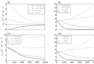
Figure 3.Sediment fluxQs as a function of distance dxas calculated by the local analytical solution (Eq. 31) at a given drainage area (A=105m2). In each panel, one parameter is varied while all others are held constant. The sediment flux coming in from upstream is an important control onQsat short length scales but declines in importance as dxapproaches 1000 m. High values of settling velocity cause lowQs, and vice versa. High sediment entrainment rates lead to highQs, as do high runoff rates. Parameter values (except where changed in the four panels) areQins =500 000 m3yr−1,V =1.0 m yr−1,Es=1.0 m yr−1, andr=1.0 m yr−1.Er=0 andφ=0 for simplicity in this case.
H (t )=H∗ln
1
(Ds/ (1−φ)) /Ebs−1
(32)
×
eDs/(1−φ)−Ebst /H∗
×
(Ds/ (1−φ))
b
Es
−1
eH0/H∗+1−1
,
where
b
Es=KsqSn−ωcs. (33)
Inspection of Eq. (32) reveals that H (t ) may become un-defined in two physically realistic situations. The first is where(Ds/ (1−φ)) /Ebs=1, and the second is whereEbs=
0. Equation (32) is therefore only applied at nodes with Ds/ (1−φ)6=Ebs andEbs>0. When Ds/ (1−φ)=Ebs, the
change in alluvium thickness with time becomes ∂H∂t =
e−H /H∗. Integrating with respect to time and applyingH= H0att=0 gives the solution forH (t )whenDs/ (1−φ)=
b
Es:
H (t )=H∗ln
K
sqSn−ωcs
H∗
t+eH0/H∗
. (34)
WhenEbs≤0, no entrainment of sediment occurs and any
changes in H (t ) are driven by deposition. In this case, changes inH are computed with a simple forward numer-ical solution:
H (t )=H0+
Ds
1−φdt. (35)
In all cases, the relevant equation forH (t ) is solved each time step using t=dt, where dt is the model time step length. Unlike forQs,H may be simultaneously calculated
at every node, allowing efficient solution of Eqs. (32)–(35) over the entire model domain. Figure 4 shows H (t ) as a function of some of the relevant variables in Eq. (32). 5.3 Calculation of change in bedrock height
(a) (b)
(c) (d)
(e) (f)
-1 -1 -1 -1
-1 -1
-1 -1
-1 -1 -1 -1
-1 -1 -1 -1
-1 -1 -1 -1
-1 -1 -1 -1
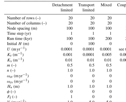
Figure 4.Bed sediment thicknessH as a function of time as calculated by our local analytical solution (general case forDs/ (1−φ)6=Ebs). In each panel, a single parameter (or set of parameters in the case ofEbs/Ds) in Eq. (32) is varied while all others are held constant.H0, the initial sediment thickness, sets the initial value of the function. The value ofH approached over long timescales is set by competition between the rates of sediment erosion and deposition, where higher sediment erosion rates drive bed sediment thickness down(a)and higher deposition rates result in greater bed sediment thickness(b). Except in the cases whereDs> Es, our local analytical solution converges on a constant value ast→ ∞. WhenDs> Es, the solution converges to a simple linear extrapolation of the deposition rate over time. Note that the adjustment time changes with different values ofEbsandDseven whenEbs/Dsremains constant(d). Parameter values (except where changed in the six panels) areH∗=1.0 m,Ds=1.0 m yr−1,Ebs=1.1 m yr−1(resulting inEs=0.95 m yr−1whenH0/H∗=2), and
H0=2.0 m.φ=0 for simplicity in this case.
R=R0+
U− KrqSn−ωcre−H /H∗
dt. (36)
The simple forward numerical solution employed in Eq. (36) becomes inappropriate at very large time steps, as H may change significantly, influencing channel slopes and there-fore bedrock erosion. However, because bedrock erosion is generally a much slower process than sediment entrainment in most cases, Eq. (36) is unlikely to introduce substantial instability.
6 Implementing SPACE in Landlab Landlab modeling toolkit
(a)
(b)
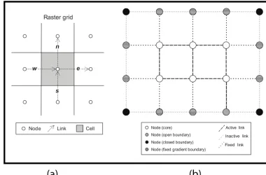
Figure 5. (a)The Landlab structured raster model grid, with definitions for major grid elements. State variables such as sediment depth and sediment flux are stored at grid nodes. While gradients such as topographic slope are calculated along links, the slope value representing the steepest descent from a node to its flow receiving neighbor is stored on the node itself. Link direction is topological; the direction of fluxes is set by gradients along links.(b)Example of possible grid setup showing the status of links and nodes. This is simply an example, not the setup of the model domain used to test the SPACE 1.0 model. The figure is reproduced from Figs. 3 and 4 in Adams et al. (2017).
components (e.g., Tucker et al., 2016; Adams et al., 2017) along with user-specific equations and functionality. The greatest advantages of using Landlab are (1) its built-in grid-ding engine, which creates model grids, efficiently stores spatially distributed variables, and handles boundary condi-tions, and (2) the ability to easily couple different compo-nents into a single model sharing a single grid. Landlab al-lows efficient coupling of components representing fluvial erosion, hillslope processes, basin hydrology (Adams et al., 2017), geodynamics, vegetation, and many other processes into novel surface dynamics models.
Landlab’s gridding engine supports grids consisting of square and rectangular grids (“raster grids”), hexagonal grids, and Voronoi–Delaunay interlocked meshes (Hobley et al., 2017). Every Landlab grid is made up of nodes, cells, and links. Nodes are points in (x, y) space. Cells are poly-gons surrounding all non-boundary (interior) nodes that may be rectangular, hexagonal, or defined by Voronoi polygons depending on the chosen grid type. Links connect adjacent pairs of nodes and are directional. Rectangular grids have four links per node, hexagonal grids have six, and Voronoi grids have a number of links per node equivalent to the num-ber of faces on each Voronoi polygon. Links have default directionality, but this directionality does not determine the directions of fluxes in Landlab models, which are set by gra-dients along links. In this paper, we focus for simplicity on
a square (1x=1y) raster grid, which is currently the only grid type supported by the SPACE model. A diagram of a generic raster grid is shown in Fig. 5. Nodes, cells, and links may all store model data in the form of NumPy arrays associ-ated with one of the three grid elements. Each data field is de-fined by a keyword in a dictionary data structure attached to a certain grid element. The SPACE model, for example, tracks sediment depth at all grid nodes, a field that may be accessed by any component (this field is called “soil depth” in Landlab to keep terminology standard between hillslope and fluvial components). An array of sediment depths at all grid nodes could be found by typinggrid.at_node[“soil__depth”]. The treatment of boundary conditions in Landlab grids is de-scribed thoroughly by Hobley et al. (2017) and Adams et al. (2017). In short, nodes may be set as “boundary” nodes and then defined as open, fixed-gradient, or closed boundaries. Non-boundary nodes are set as “core” nodes.
7 Verification and evaluation: comparison to analytical solutions for detachment-limited, transport-limited, and mixed cases
model behavior. In this section, we compare the behavior of the SPACE 1.0 Landlab component (the numerical imple-mentation of the SPACE model equations presented above) to steady-state analytical solutions for standard detachment-limited and transport-detachment-limited models to assess whether our numerical implementation of the SPACE algorithm can repli-cate these two end-member cases. In addition, we test the performance of the SPACE component against steady-state analytical solutions for a mixed case where both bedrock ero-sion and sediment transport influence channel evolution. For the three test cases, we use a simple 20×20 node square raster grid with dx=100 m, for a 2 km×2 km model do-main. The initial topography of the domain is a plane tilted to the lower left (southwest) corner with random microscale roughness to force flow convergence. The lower left cor-ner is the only open boundary and is therefore the basin outlet in all cases. Such a setup results in a model domain that drains to the single open boundary node, allowing pre-dictable drainage network development. The random seed is held constant so that all runs start from the same initial topog-raphy. For simplicity in these test cases, there are no other surface process models (e.g., hillslope models) coupled to the SPACE component. While the SPACE 1.0 component is stable at 10-year time steps under most conditions, we use a time step of 1 year here to maximize numerical accuracy for comparison with analytical solutions. We run the model for 100 000 years for the detachment- and transport-limited com-parisons, and 200 000 years for the mixed bedrock–alluvial comparison (see Table 1). We define steady state as having been achieved when every interior (non-boundary) node is lowered at the same rate as the base-level node to within 10−6m yr−1precision but allow the model to run for the full
imposed run time even after steady state has been achieved. 7.1 Detachment-limited comparison
With no sediment (H=0 and cs=0) and Ff=1 (all
bedrock eroded becomes wash load and is not included in model calculations), all changes in bed elevation are driven by changes in bedrock elevation:
∂η ∂t =
∂R
∂t , (37)
where ∂R
∂t =U− KrqS
n−ω
cr. (38)
When ωcr=0, Eq. (38) is the simple stream power model
(Whipple and Tucker, 1999). At topographic steady state, when ∂R∂t =0 and U=KrqSn, the slope at every point in
the channel is
S=
U Krq
1/n
. (39)
Table 1.Parameter values for SPACE model test cases.
Detachment Transport Mixed Coupled limited limited
Number of rows (–) 20 20 20 50
Number of columns (–) 20 20 20 50
Node spacing (m) 100 100 100 100
Time step (yr) 1 1 1 1
Run time (kyr) 100 100 200 300
InitialH(m) 0 100 0 0
U(m yr−1) 0.0001 0.0001 0.0001 see text
Kr(m−1) 0.001 0.0001 0.005 0.0001
Ks(m−1) 0.01 0.01 0.01 0.0005
m(–) 0.5 0.5 0.5 0.5
n(–) 1.0 1.0 1.0 1.0
ωcr(m yr−1) 0 0 0 0
ωcs(m yr−1) 0 0 0 0
H∗(m) 1.0 1.0 1.0 1.0
φ(–) 0 0 0 0
Ff(–) 1 0 0 0
V (m yr−1) 1.0 5.0 5.0 2.0
Not all parameters will influence the model outcome in all cases. For example, the value ofVis irrelevant for the detachment-limited case when all eroded bedrock passes out of the model domain as permanently suspended fine sediment (Ff=1).
Because we use a simple stream power formulation where q=kqAmfor our test case, the slope–discharge relationship
may be rewritten to yield a slope–area relationship:
S=
U
KrAm
1/n
, (40)
wherekq is subsumed intoKr. We test whether the SPACE
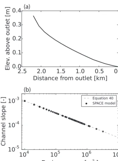
component can replicate steady-state detachment-limited be-havior by comparing slope–area relationships predicted by Eq. (40) with those calculated by the SPACE component. See Table 1 for the parameter values used. Figure 6 shows the results after the test model domain has achieved topo-graphic steady state. Figure 6a shows the longitudinal pro-file of the longest drainage path in the model domain. As predicted by the theory described above, slope and drainage area trade off such that the outcome is a concave-up lon-gitudinal profile with constant concavity. Figure 6b com-pares the slope–area relationship predicted by Eq. (40) (gray dashed line) to the slope–area relationship in the steady-state model landscape (black dots). All core nodes from the model domain are shown, and every node obeys the pre-dicted detachment-limited slope–area scaling. The slope of the slope–area power-law scaling relationship (Fig. 6b) is the channel concavity, thus confirming that the channel concav-ity observed in the longitudinal profile is constant, and that the SPACE component agrees with theoretical predictions for detachment-limited rivers at steady state.
7.2 Transport-limited comparison
When sediment thicknessH is large relative toH∗, changes
(a)
(b)
Figure 6. (a) Longitudinal profile of the longest channel in the model domain under detachment-limited conditions, showing that the channel is in equilibrium with the imposed base-level fall, and that the SPACE component yields concave-up longitudinal profiles at steady state.(b)Comparison between the SPACE component and Eq. (40) (steady-state slope–area relationship under detachment-limited conditions). The numerical implementation of the SPACE component successfully replicates the predicted power-law slope– area relationship.
bed elevation, which is set by the balance between sediment erosion, deposition, and rock uplift:
∂η
∂t =U+Ds−Es. (41)
At steady state, ∂η∂t =0 andEs−Ds=U. Substituting in the
equations derived above for sediment erosion and deposition and assuming for simplicity that sediment porosityφand the sediment erosion thresholdωcsare negligible,
KsqmSn−V
Qs
Q =U. (42)
Applying the steady-state mass conservation relationship (Qs=U A), recalling thatQ=rA, and solving forS gives
an expression for steady-state channel slope:
S=
U V
Ksqr
+ U
Ksq
1/n
. (43)
Ifq=kqAmas in our test case, the resulting slope–area
re-lationship is then
S=
U V
KsAmr
+ U
KsAm
1/n
, (44)
wherekqis subsumed intoKs. Equation (44) nicely
distin-guishes the contributions of sediment deposition (first term on the right side) and sediment entrainment (second term on the right side) to steady-state channel slope. If effective settling velocity is negligible, erosion is only limited by the efficiency of sediment entrainment and Eq. (44) gives the detachment-limited steady-state slope (though importantly the bed is still entirely composed of sediment). If entrain-ment and deposition of sedientrain-ment are rapid enough that ero-sion is limited by transport capacity (i.e., the river has enough energy to erode more sediment but the water column is satu-rated), the system is transport limited and the left-hand term in Eq. (44) dominates in setting the steady-state slope. Note the subtle difference between Eqs. (44) and (18); whenH
H∗ and all surface lowering is accomplished by sediment
entrainment, both terms on the right-hand side of Eq. (44) reflect erosion of sediment (i.e., Ks is used in both). This
occurs because whenHH∗, change in bedrock elevation
over time is not zero as in the true complete steady state but is equal to the uplift rate. Therefore, for topographic steady state to be achieved, both the transport and detachment terms of Eq. (44) must be accomplished through erosion of sedi-ment. Equation (44) may be rewritten to show that it predicts a standard stream power slope–area relationship that is mod-ified by the ratio of settling velocity to effective runoff:
S=
V r +1
1/n
U Ks
1/n
A−m/n. (45)
We compare the slope–area relationships predicted by Eq. (44) with those extracted from the SPACE model. In order to achieve conditions in which the transport term in Eq. (44) dominates, we set initial soil depth to 100 m every-where on our test grid so thatHH∗. See Table 1 for all
parameter values.
Figure 7 shows the results of the transport-limited model experiment. Figure 7a shows the longitudinal profile of the longest channel and shows that the SPACE component pro-duces concave-up longitudinal profiles at steady state un-der transport-limited conditions. The appearance of constant concavity in the longitudinal profile is verified by the con-stant slope in log–log space of the slope–area data shown in Fig. 7b. Figure 7b compares the theoretical slope–area rela-tionship (Eq. 44, gray dashed line) with data from the model run (black dots). All core nodes from the model domain are included, and all agree well with the theoretical prediction. In addition to matching the analytical prediction for chan-nel slope, the model also matches the expected steady-state sediment flux relationship, Qs=U A (Fig. 7c). This
(a)
(b)
-1
(c)
Figure 7. (a) Longitudinal profile of the longest channel in the model domain under transport-limited conditions, showing that the channel is in equilibrium with the imposed base-level fall, and that the SPACE component yields concave-up longitudinal profiles at steady state. (b) Comparison between the SPACE component and Eq. (44) (steady-state slope–area relationship under transport-limited conditions). The numerical implementation of the SPACE component successfully replicates the predicted power-law slope– area relationship. (c)Sediment fluxQs as a function of drainage area. The model matches the predicted linear relationship (Qs= U A).
expected transport-limited model behavior for both slope and sediment flux at steady state.
7.3 Mixed bedrock–alluvial comparison
One major advantage of SPACE over many existing fluvial erosion models is its ability to simultaneously compute the evolution of an alluvial layer and a bedrock surface. True steady state in the mixed bedrock–alluvial case occurs when the thickness of the alluvial layerH and the bedrock height Rare both unchanging in time (∂H∂t =0 and ∂R∂t =0). In such a scenario,Es=Ds andU=Er. As described in Sect. 4.5,
steady-state analytical solutions exist for channel slope, sed-iment thickness, and sedsed-iment flux (here, again, we useq=
kqAmwithkqsubsumed intoKsandKr, and keepφ=0 and
Ff=0):
S=
U V
KsAmr
+ U
KrAm
1/n
, (46)
H= −H∗ln "
1− V
Ksr
Kr +V
#
, (47)
and
Qs=U A. (48)
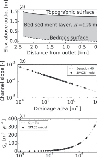
Running the SPACE component to complete steady state in a case where both sediment entrainment and bedrock erosion contribute to setting channel slope should therefore result in a concave-up channel profile with a sediment layer of constant thickness, and sediment flux equal to the product of the rock uplift rate and drainage area. We use the same tilted plane ini-tial model domain as described in Sect. 7 to test whether the model can replicate the expected behavior in the bedrock– alluvial case. Matching the steady-state analytical solutions requires both erosion of bedrock to generate the concave-up profile and accumulation of sediment to a constant thickness over the landscape. We begin the numerical experiment with zero sediment thickness at all nodes. Table 1 shows all pa-rameter values used. The driver script used for this model experiment is included in the code guide for this paper.
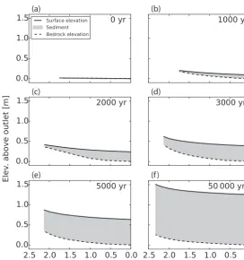
Figure 8 shows the evolution of the longitudinal bedrock profile and alluvial cover layer in the longest channel over several model time slices. Beginning from a low-slope tilted plane, the channel incises bedrock and begins to build up a layer of alluvium on the channel bed. As model time pro-gresses, the channel profile increases in concavity and the layer of alluvium thickens. Alluvial thickening progresses from downstream to upstream. By the final time slice, the alluvial layer has reached its equilibrium value, the channel profile has equilibrated to the imposed uplift rate, and the bedrock surface, alluvium thickness, and topographic sur-face are all at steady state. Figure 9a shows the final chan-nel profile when the topographic surface, sediment thick-ness, and bedrock height are all at steady state. The to-pographic surface (top of the sediment layer) is parallel everywhere to the bedrock surface, and the bed sediment layer is 1.25 m thick at every point along the channel pro-file. GivenV =5 m yr−1, Ks=0.01, andKr=0.005 m−1,
as used in the model, the steady-state sediment thickness of H=1.25 m calculated by the model matches the analytical prediction of Eq. (47). Figure 9b compares the theoretical prediction for slope–area scaling given by Eq. (46) (gray dashed line) with the model results (black dots). As in the detachment-limited and transport-limited cases, the model matches the analytical prediction. Figure 9c compares the theoretical steady-state relationship between drainage area and sediment flux (Qs=U A) with modeled sediment flux
(a) (b)
(c) (d)
(e) (f)
Figure 8.Time series of longitudinal profile evolution for the longest channel in the test model domain as the domain is uplifted relative to base level. Profile distance lengthens over time as the original tilted ramp is incised; horizontal scale on all plots is the same.(a)Initially (0 yr), the channel topographic surface is effectively flat with zero sediment thickness.(b)By 1000 yr, a slightly concave-up bedrock profile has developed, with a thin, downstream-thickening layer of bed sediment resulting in a surface profile that is less concave-up than the bedrock profile. (c–e)Over the following three time slices, continued rock uplift relative to base level causes increased concavity in the bedrock profile, as well as continued thickening of the sediment layer. The sediment layer thickens in a downstream to upstream progression.
(f)By 50 000 yr, the sediment layer has uniform thickness, resulting in a surface profile of equal concavity to the bedrock profile, and the alluvial layer thickness, topographic surface elevation, and bedrock surface elevation are all equilibrated to the imposed rock uplift rate and are therefore unchanging in time. Vertical exaggeration≈1100×.
in Qs with drainage area. The ability of the SPACE
com-ponent to treat both the detachment-limited and transport-limited end-members of fluvial systems as well as the mixed bedrock–alluvial case confirms that the model equations are being solved correctly, and importantly that our use of sta-bilizing, local analytical solutions does not compromise the ability of the model to replicate expected behavior. Below, we show how the SPACE component may be efficiently cou-pled with other surface process models in the Landlab mod-eling framework to provide insight into landscape evolution.
8 Application to landscape evolution modeling: coupling SPACE with hillslope diffusion to model topographic growth and decay
One frequent application of landscape evolution modeling is the exploration of landscape response to tectonic perturba-tions. Understanding the growth and decay of topography has significant implications for interpretation of the stratigraphic
record, which is composed of sediment that is detached and transported from upland landscapes. In this section, we show how the SPACE component can be coupled with a hillslope diffusion model in the Landlab modeling toolkit to simulate landscape response to changing rock uplift rates. In addition to computing topographic change that incorporates both sed-iment and bedrock surface evolution, we show the capability of the SPACE component to provide information about sedi-ment fluxes delivered from the model catchsedi-ment over time. 8.1 Model setup