https://doi.org/10.5194/gmd-10-3309-2017 © Author(s) 2017. This work is distributed under the Creative Commons Attribution 3.0 License.
The Gravitational Process Path (GPP) model (v1.0) – a GIS-based
simulation framework for gravitational processes
Volker Wichmann1,2
1alpS, Centre for Climate Change Adaptation, 6020 Innsbruck, Austria 2Laserdata GmbH, 6020 Innsbruck, Austria
Correspondence to:Volker Wichmann ([email protected]) Received: 7 January 2017 – Discussion started: 15 February 2017
Revised: 21 July 2017 – Accepted: 10 August 2017 – Published: 8 September 2017
Abstract. The Gravitational Process Path (GPP) model can be used to simulate the process path and run-out area of grav-itational processes based on a digital terrain model (DTM). The conceptual model combines several components (pro-cess path, run-out length, sink filling and material deposition) to simulate the movement of a mass point from an initiation site to the deposition area. For each component several mod-eling approaches are provided, which makes the tool config-urable for different processes such as rockfall, debris flows or snow avalanches. The tool can be applied to regional-scale studies such as natural hazard susceptibility mapping but also contains components for scenario-based modeling of single events. Both the modeling approaches and precur-sor implementations of the tool have proven their applicabil-ity in numerous studies, also including geomorphological re-search questions such as the delineation of sediment cascades or the study of process connectivity. This is the first open-source implementation, completely re-written, extended and improved in many ways. The tool has been committed to the main repository of the System for Automated Geoscien-tific Analyses (SAGA) and thus will be available with every SAGA release.
1 Introduction
Rapid mass movements such as rockfall, debris flows or snow avalanches are common features in mountainous re-gions. Due to population growth and the advancing construc-tion of infrastructure and buildings in such areas, rapid mass movements pose more and more of a risk to society and can result in severe damages or even disasters. Besides early
warning systems and protection measures for disaster pre-vention, hazard susceptibility zoning, which identifies po-tentially endangered areas, is required for risk analysis and the creation of hazard maps (Carrara et al., 1991; Fell et al., 2008; Hu et al., 2016).
dis-tances (Lied and Bakkehøi, 1980; Hungr and Evans, 1988; Dorren, 2003; Zimmermann et al., 1997). Other approaches, often based on the mass flow model of Voellmy (1955), are using simplified physically based models considering only the center of mass but not its deformation (Körner, 1976; Perla et al., 1980; Hegg, 1996; Gamma, 2000; Wichmann and Becht, 2005; Horton et al., 2013).
This paper introduces the Gravitational Process Path (GPP) model version 1.0, an attempt to provide a GIS-based modeling framework for the simulation of process path and run-out area of gravitational processes. The GPP model is a conceptual model, concatenating components for process path determination, run-out calculation, sink filling and ma-terial deposition. For each of these components, several well established modeling approaches are implemented and can be chosen by the user. This makes the GPP model config-urable for different processes like rockfall, debris flows or avalanches.
Basically, the GPP model simulates the movement of a mass point over a raster DTM from an initiation site to the deposition area. Therefore it includes empirical, stochastic and physically based modeling approaches and provides the option of terrain modification by material deposition during operation. Although some of the implemented approaches are based on simplifying concepts, realistic results can be achieved with the great advantage of requiring only a few input parameters. This makes it possible to use the tool for regional-scale studies, but it also includes some components for scenario modeling of single events. The approaches im-plemented in the model components have been successfully used for hazard susceptibility mapping (e.g., Zimmermann et al., 1997; Heinimann et al., 1998; Wichmann and Becht, 2004; Mergili et al., 2015; Proske and Bauer, 2016) and ge-omorphological process studies, e.g., on sediment cascades or process connectivity (e.g., Wichmann et al., 2009; Haas et al., 2012a; Heckmann and Schwanghart, 2013; Heckmann et al., 2016).
For process path modeling, the GPP model includes the single-flow-direction path-finding approach of O’Callaghan and Mark (1984), also known as the D8 flow direction ap-proach (Jenson and Domingue, 1988), which has been used in various hydrological and geomorphological applications. Furthermore, a random walk approach as introduced in the dfwalk model by Gamma (1996, 2000) is implemented. It is especially suited for process path delineation of gravita-tional processes and has been used by various authors for rockfall modeling (e.g., Wichmann and Becht, 2006; Haas et al., 2012b; Proske and Bauer, 2016), debris flow model-ing (e.g., Zimmermann et al., 1997; Heinimann et al., 1998; Wichmann, 2006; Mergili et al., 2015) and avalanche model-ing (e.g., Heckmann, 2006; Schmidtner, 2012).
For run-out distance calculation, the GPP model in-cludes several approaches based on the energy line prin-ciple (e.g., Heim, 1932; Hungr and Evans, 1988), which have been applied to various processes including
rock-fall (e.g., Heinimann et al., 1998; Dorren, 2003), de-bris flows (e.g., Zimmermann et al., 1997) and avalanches (e.g., Körner, 1980). Furthermore, the one-parameter fric-tion model of Scheidegger (1975) is implemented, which has been used for rockfall run-out calculations in several studies (e.g., van Dijke and van Westen, 1990; Meißl, 1998; Dor-ren and Seijmonsbergen, 2003; Wichmann and Becht, 2005; Haas et al., 2012b). Finally, the run-out model of Perla et al. (1980), often referred to as PCM model, is included. The PCM model has been applied for avalanche run-out modeling by, for example, Körner (1976), Hegg (1996) and Heckmann (2006). It has also been applied to model debris flows (Rick-enmann, 1990; Zimmermann et al., 1997; Heinimann et al., 1998; Gamma, 2000; Wichmann, 2006; Mergili et al., 2012, 2015) and large rock slides (e.g., Körner, 1976).
The GPP model is the first open-source implementation based on previous work of the author, but it is completely re-worked and enhanced in various aspects. It is implemented as a tool for the System for Automated Geoscientific Anal-yses (SAGA; Conrad et al., 2015) and is released as free open-source software (licensed under the GPL). The source code has been committed to the main repository of SAGA hosted at sourceforge.net (https://sourceforge.net/projects/ saga-gis/), and binaries are available with every SAGA re-lease.
The paper is structured as follows: Sect. 2 provides an overview of the framework and the model components (pro-cess path, run-out, sink filling and deposition). The individ-ual modeling approaches implemented for each component are described in detail in Sect. 3. In Sect. 4 model config-urations and application examples for rockfall, debris flow, avalanche and scenario modeling are presented. Finally a dis-cussion and conclusion is provided.
2 General model structure
The GPP model is intended to provide a software framework for gravitational process path modeling. It integrates com-ponents for process path determination, run-out calculation, sink filling and material deposition. For each of these com-ponents, several modeling approaches are implemented. This makes it possible to concatenate modeling approaches as re-quired to simulate the behavior of a certain geomorphologi-cal process or to use suitable approaches with regard to the available input data.
Initialize Update Update
particle
-I
path speed
l
l
DTM Stop No
border
Ives res
Next particle
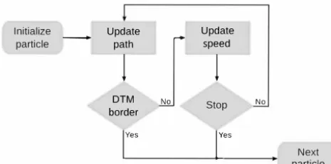
Figure 1.Flowchart of a basic GPP model configuration for mod-eling on a regional scale.
The GPP model computes several model realizations for each start cell (Monte Carlo simulation). The number of model iterations is defined by the user (default: 1000 itera-tions). The overlay of the model results from all iterations shows the final model result, i.e., the complete process area (and not individual process paths), as every iteration will show a different result because of the stochastic components in the model.
Besides the components for process path and run-out cal-culation, the GPP model integrates components, which can modify the DTM in each model iteration by material depo-sition: there is a model component, which handles natural or artificial sinks, and a component to deposit material on pro-cess stop or along the propro-cess path. This allows the model to overcome sinks or to simulate the blocking of a channel by wood and debris. In order to use these components, the GPP model requires an input data set with material heights per start cell.
Figure 1 shows a basic setup, usually used for gravitational process path modeling on a regional scale. As this setup does not include the filling of sinks, a hydrologically sound DTM must be used. In each model iteration, a particle is initialized using information from its start cell. In a first step, one of the process path models is used to update the particle’s path. In the case that there is no valid process path cell, i.e., the path has reached the border of the DTM or a NoData cell, the par-ticle is deleted and the next parpar-ticle is initialized. If the next cell in the process path can be determined, one of the run-out models is used to update the speed of the particle, or, in the case of an approach based on the energy line principle, the respective angle criterion is checked. In the case in which the particle has stopped, the next particle is initialized. Oth-erwise, the next cell of the process path is determined.
A model configuration including the filling of sinks is de-picted in Fig. 2. This setup requires additional information on the material available per start cell. In the case that the process path has ended up in a sink, the amount of material available for the particle is checked. This amount of material is then used to fill up the process path upslope while preserv-ing a downward slope, allowpreserv-ing the next particle to overcome
the sink. In the case that the material available in an iteration is not enough or the sink is larger, several model iterations might be necessary to completely fill up the sink. After the attempt to fill the sink, the next particle is initialized.
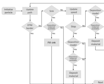
Figure 3 shows a fully featured setup of the GPP model, which is usually used for scenario modeling of a single (or a small number of) events. In this setup, material may be posited when a particle stops, depending on the chosen de-position model and whether there is (still) material available for the particle. Then the next particle is initialized. In the case that the particle has not stopped, it depends again on the chosen deposition model and the available material whether material is deposited along the process path or not. Then the next cell of the process path is determined. The deposition of material on stopping or based on slope and velocity along the process path alters the terrain between successive model iterations.
The sequence in which release areas, as well as particles, are initialized is crucial when material deposition is simu-lated. The modification of the terrain between model itera-tions can influence process paths and run-out distances sig-nificantly. The following processing orders are implemented: a. Release areas in sequence: the release areas are pro-cessed one by one; in each model iteration, all start cells of a release area are processed in ascending order of their elevation. This configuration computes all model iterations for the start cells of release area one, then for the start cells of release area two and so on.
b. Release areas in sequence per iteration: the release ar-eas are processed one by one in each model iteration; the start cells are processed in ascending order of their elevation. This configuration computes a single model iteration with the start cells of release area one, then with all start cells of release area two and so on; the next model iteration is then run over all release areas. c. Release areas in parallel per iteration: in each model
it-eration the start cells of all release areas are processed in ascending order of their elevation. With this configura-tion, all start cells are processed in each model iteration sorted by elevation, irrespective of their membership to a certain release area.
Initialize
particle
Next particle
Figure 2.Flowchart of a GPP model configuration making use of the sink-filling approach.
Figure 3.Flowchart of a fully featured GPP model configuration for scenario modeling.
3 Modeling approaches
Within the following sections, the modeling approaches cur-rently implemented for each model component are described in detail. The user can choose which model should be used in each component and combine them to simulate various pro-cesses. Typical model configurations are presented in Sect. 4.
3.1 Process path modeling approaches
3.1.1 Maximum slope
This approach, as proposed by O’Callaghan and Mark (1984), is implemented mainly for convenience in order to provide a simple means to detect the process path along the gradient of gravity. A particle follows the steepest descent of the slope:
n=max{(z−zi)/di}, (1) wherenis the neighbor of steepest descent,zis the elevation of the currently processed cell,ziis the elevation of neighbor celli, anddiis the horizontal distance to neighbor celli.
The model result is thus deterministic, with the exception of its behavior (as implemented in the GPP model) when two or more neighbor cells show the same steepest descent or when a flat area is reached. In the first case, one of the neigh-bor cells is chosen at random. On flat areas a set of potential neighbor cells is determined which is made up of all neigh-bors with the same elevation as the current cell which have not been traversed yet in the current model iteration. From this set, a process path cell is chosen at random. This intro-duces a probabilistic component. Further, the terrain could have been modified between two model iterations by sink filling or material deposition.
The Maximum Slope model approach has no special pa-rameters besides those controlling the mode of operation of the GPP model main loop, such as the number of model rep-etitions or the processing order. The pseudo-random number generator, used to choose a neighbor cell at random under the predescribed conditions, can be initialized either with the current time or a fixed seed value. The latter will always pro-duce the same succession of values for a given seed value and will thus give the same results for consecutive tool runs. 3.1.2 Random walk
With this approach, the process path is modeled by a variant of the dfwalk model as proposed by Gamma (1996, 2000). It uses a stochastic way of path finding, which makes it possible to model the lateral spreading of a process by calculating sev-eral iterations from the same start position. Besides the pa-rameters controlling the Monte Carlo simulation, such as the number of repetitions, theRandom Walkapproach has three parameters to calibrate the model in order to mimic the be-havior of different geomorphological processes: (i) a thresh-old parameter defines the terrain slope below which diver-gent flow is allowed; (ii) this is accompanied by an exponent for divergent flow: below the slope threshold, the parameter controls the degree of divergence; (iii) finally, a persistence factor can be used to preserve the direction of movement by weighting the current flow direction in order to account for inertia, which can be observed for debris flows or wet snow avalanches (Nohguchi, 1989; Takahashi et al., 1992). Rockfall may be modeled with (almost) no persistence and a higher degree of divergence.
For the currently processed grid cell, a setNof potential flow path cells is determined from all immediate neighbor cells in a 3 by 3 window, which have an equal or lower eleva-tion than the central cell. This is done in several steps. First of all, for each neighbor cellia slope valueγi, based on the slope thresholdβthres, is calculated (Gamma, 2000):
γi= tanβi tanβthres
, βi ≥0, i∈ {1,2, . . .8}, (2) whereβi is the slope to neighbor celli. The maximum value
γmax=max{γi}is a measure of how close the slope to the steepest neighbor is to the slope threshold. In the case that
γmax>1 the setNof potential flow path cells is only made up of the steepest neighbor. Otherwise, themfdf(multiple flow directions for debris flows; Gamma, 2000) criterion is used to decide which neighbor cells are additionally included in N:
γi≥(γmax)a (0< γmax≤1, a≥1) , (3) wherea is the exponent to control the amount of divergent flow (a≥1). Ifγi is greater than or equal to themfdf crite-rion, then the neighboriis included inN. Thus, the setNis given by (Gamma, 2000):
N= {i|γi≥(γmax)afori∈ {1,2, . . .8}} (4a) if 0< γmax≤1 and
N= {i|γi=γmaxfori∈ {1,2, . . .8}} (4b) ifγmax>1.
The slope threshold makes it possible to adjust the model to different topography: in steep sections of the process path, where the terrain slope is near the threshold, only steep neighbors are allowed in addition to the steepest descent. In flat sections, almost all lower neighbor cells are poten-tial flow path cells and the tendency for divergent flow is in-creased. The degree of divergent flow below the slope thresh-old can be controlled by the exponent of divergent flow. This sensitivity to the terrain conditions is an important property which is missing in the modeling approaches developed for hydrological processes, which distribute the flow proportion-ally to the slope to all lower neighbors irrespective of the local topography (Gamma, 2000).
Finally, a cell is picked at random from the setN. The probability for each cell probi is given by
probi= fi·tanβi P
jfj·tanβj
, (5)
whereidescribes the currently processed neighbor cell,j de-picts all neighbor cells in setN, andf is a weighting factor. In the case that the flow direction to neighboriequals the pre-vious flow direction,f equals the persistence factorp(with
to weight the current flow direction, which results in a higher probability that the neighbor in this direction gets selected. This property can be used to reduce abrupt changes in flow direction. Finally the transition probabilities are scaled to ac-cumulated values between 0 and 1, and the pseudo-random generator is used to select one flow path cell from the set.
In the GPP model, the approach is extended to also handle flat areas. This is done as described for theMaximum Slope approach with the same restriction that a potential successor cell must not have been traversed yet in the current model iteration in order to prevent endless loops.
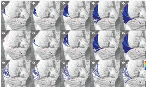
The result of several model iterations is a raster data set storing the transition frequencies, i.e., how many times a grid cell has been traversed. Figure 4 shows the effect of different parameter settings for the three calibration parameters slope threshold, exponent for divergent flow and persistence factor (the run-out length was calculated with theGeometric Gradi-entapproach using an angle of 26.5◦; see Sect. 3.2.1, point a).
The number of model iterations is set to 1000 in the exam-ples (a) to (j). In Fig. 4a–e the slope threshold (40◦) and the persistence factor (1.0) are fixed, while the exponent for di-vergent flow is increased in several steps (1.0, 1.1, 1.2, 1.5 and 2.0). It is obvious that the extent of the process area in-creases significantly because of the higher degree of lateral spreading.
In Fig. 4f–j the exponent for divergent flow (1.5) and the persistence factor (1.0) are fixed, while the slope threshold is increased gradually (15◦, 20◦, 30◦, 40◦ and 60◦). It can be seen that the point at which lateral spreading is allowed is moving up the torrential fan, resulting in an increase of the total process area.
Figure 4k–o show the results of a stepwise increase of the persistence factor (1.0, 1.5, 2.0, 2.5 and 3.0) while the slope threshold (40◦) and the exponent of divergent flow (2.0) are fixed. Here, only a single iteration was calculated from each start cell in order to visualize single trajectories. It is obvious that with higher persistence factors the number of changes in direction along a trajectory is decreasing.
3.2 Run-out modeling approaches
In order to determine the run-out length of a particle, several approaches are implemented in the GPP model. These range from rather simple but convenient approaches (regarding, for example, the comparison with field observations) based on the energy line principle to one- and two-parameter friction models. In the following, these approaches are described in detail.
3.2.1 Energy line approaches
The run-out length of a process is often described by the ver-tical and horizontal distances covered by a particle from its start to the stopping position:
tanα=dv/dh, (6)
whereαis the angle to the horizontal and dvand dhare the vertical and horizontal offset, respectively. Both offsets can be defined differently, see below. This describes a straight en-ergy line from the start to the stopping position (Heim, 1932). With a straight energy line, the velocity can be calculated by Körner (1980):
vi=
p
2·g·hv, (7)
wherevi is the velocity (m s−1) on the currently processed grid cell,gis the acceleration due to gravity (m s−2), andh
v is the height difference (m) between the energy line and the current grid celli. Although the angleα is not constant, it can be observed that it has a characteristic value range for gravitational movements of a specific type. The calibration of the angleα, which can be measured quite easily, is usu-ally done by field observations and mapping. All approaches based on the energy line principle provide the possibility to output raster data sets storing the stopping positions and the maximum velocity encountered in each cell of the process path.
a. Geometric gradient: The geometric gradient (Heim, 1932) defines the vertical offset as the vertical distance between the release area and the end of the deposit. The horizontal offset is defined as the horizontal distance be-tween these two points. This modeling approach thus re-quires just the friction angleαas input. The GPP model supports both a global friction angle or a raster data set with friction angles for each start cell. Once the angle between the start cell of the particle and the current po-sition of the particle drops below the friction angleα, the end of the deposit is reached.
b. Fahrböschung: For the Fahrböschung principle (Heim, 1932) the vertical offset is determined in the same way as for the geometric gradient. But the horizontal offset is not defined as the horizontal distance between start and end point but as the length of the horizontal projection of the actual process path. Again, the friction angle can be provided either as a global value or by a raster data set with friction angles for each start cell.
Figure 4.Effect of different random walk parameter settings;(a)–(e)different exponents for divergent flow (1.0, 1.1, 1.2, 1.5 and 2.0); (f)–(j)different slope thresholds (15◦, 20◦, 30◦, 40◦and 60◦);(k)–(o)different persistence factors (1.0, 1.5, 2.0, 2.5 and 3.0). For details see text.
The shadow angle can again be provided either as a global value or by a raster data set with shadow angles for each start cell. In order to determine the location of the first impact of a particle on the talus slope, the GPP model implements two different approaches: (i) the user provides a raster data set with impact areas. Once a particle reaches a cell labeled as impact area, the location of this cell is used to measure the shadow angle; (ii) a threshold describing the slope angle above which free fall is assumed is provided. As soon as the angle between the start cell and the current position of the particle drops below the threshold, the location of this cell is used to measure the shadow angle.
3.2.2 One-parameter friction model
The one-parameter friction model has been developed to simulate rockfall and is based upon concepts introduced by Scheidegger (1975), which have been extended by various authors (van Dijke and van Westen, 1990; Meißl, 1998; Dor-ren and Seijmonsbergen, 2003). The GPP model implements several of these approaches, more details can be found in Wichmann and Becht (2005) and Wichmann (2006). The one-parameter friction model calculates the velocity of the currently processed grid cell according to the velocity on the previous cell of the process path, the slope and a friction
pa-rameter. Once the velocity becomes zero, the end of the de-posit is reached. Once a block is detached from the rock face, it is falling in free air:
vi=
p
2·g·hf, (8)
wherevi is the velocity (m s−1) on the currently processed grid cell,gis the acceleration due to gravity (m s−2), andhf is the height difference (m) between the start cell and the cur-rent grid celli. The impact on the talus slope occurs, similar to the shadow angle model, if (a) a particle reaches a cell la-beled as impact area or (b) the angle between the start cell and the current position of the particle drops below the free fall threshold. The decrease of velocity on the talus slope due to energy loss on the first impact can be calculated in two dif-ferent ways:
i. energy reduction (Scheidegger, 1975):
vi=
p
2·g·hf·K, (9)
ii. preserved component of velocity (Kirkby and Statham, 1975):
vi=
p
2·g·hf·sinβi, (10)
whereβi denotes the local slope gradient (◦). Here, the component of the fall velocity parallel to the talus slope surface is conserved.
Approach (i) requires the user to specify the amount of en-ergy reduction as calibration parameter. Approach (ii) usu-ally results in larger run-out distances. The strong depen-dence of approach (ii) on the slope of the impact cell compli-cates the model calibration (Wichmann, 2006). Approach (i) is used as the default in the GPP model. After the impact, two different modes of motion can be modeled (Scheideg-ger, 1975):
i. sliding:
vi=
q
v2(i−1)+2·g·(h−µs·D), (11)
wherev(i−1)is the velocity (m s−1) on the previous grid cell of the process path, his the height difference (m) between adjacent grid cells,Dis the horizontal differ-ence (m) between adjacent grid cells, andµsis the slid-ing friction coefficient (–).
ii. rolling:
vi=
q
v2(i−1)+10/7·g·(h−µr·D), (12) whereµris the rolling friction coefficient (–).
Once the velocity on a grid cell becomes zero, the end of the deposit is reached. The model calibration usually requires only two parameters: the amount of energy loss on impact (%) and, depending on the chosen mode of motion, either the sliding or the rolling friction coefficient (–). The friction coefficient can be provided as a global value or spatially dis-tributed by providing a raster data set with friction values. Impact on the talus slope can be modeled either by providing an input raster data set with impact areas or by using a slope threshold (see Sect. 3.2.1, point c). Besides the possibility to output a raster data set storing the stopping positions, a raster data set with the maximum velocity encountered in each cell of the process path can be output.
3.2.3 PCM model
The PCM model (Perla et al., 1980) is a two-parameter fric-tion model originally developed to calculate the run-out dis-tance of avalanches. It is based on the model of Voellmy
(1955). The model has also been applied to debris flows by various authors (Rickenmann, 1990; Zimmermann et al., 1997; Gamma, 2000; Wichmann, 2006). It is a center-of-mass model and it is assumed that the motion is mainly gov-erned by a sliding friction coefficientµand a mass-to-drag ratioM/D. In steeper parts of the process path, the veloc-ity is mainly influenced byM/D, whereas the velocity in the run-out area is dominated byµ. The velocity on the currently processed grid cell depends on the velocity of the previous cell, the slope, the slope length and the two friction coeffi-cients:
vi=
q
αi·(M/D)i· 1−eβi
+ v(i−1) 2
·eβi (13)
and
αi=g (sinθi−µicosθi) , (14)
βi=
−2Li
(M/D)i, (15)
wherevi is the velocity (m s−1) on the currently processed grid cell,gis the acceleration due to gravity (m s−2),θis the local slope (◦),L is the slope length between adjacent grid cells (m),µis the sliding friction coefficient (–), andM/Dis the mass-to-drag ratio (m). Perla et al. (1980) assume the fol-lowing velocity correction forv(i−1) beforevi is calculated in the case of a concave transition in slope direction:
v(i∗−1)=
v(i−1)cos θ(i−1)−θi
ifθ(i−1)≥θi
v(i−1) ifθ(i−1)< θi.
(16) The correction is based on the conservation of linear mo-mentum and has a higher magnitude in the event of abrupt transitions. The accurate stopping position on a grid cell may be calculated by the following:
s=(M/D)i
2 ln 1−
(vi−1)2
αi(M/D)i
!
, (17)
wheres is the length (m) of the process path segment on the grid cell. In the GGP model,sis not calculated and the process stops as soon as the square root in Eq. (13) becomes undefined. Thus the raster cell size determines the precision of the stopping position, which is a reasonable compromise for a grid-based model.
Gamma (2000) proposed incorporating the velocity cor-rection (Eq. 16) directly into the velocity calculation (Eq. 13):
vi= (18)
q
αi·(M/D)i· 1−eβi
+
v(i−1) 2
·eβi·cos(1θi) and
1θi =
θ(i−1)−θi ifθ(i−1)> θi 0 ifθ(i−1)≤θi
In the GPP model Eq. (18) is implemented. The model has to be calibrated by the friction parametersµandM/D. In or-der to overcome the problem of mathematical redundancy – various combinations of the two parameters can result in the same run-out distance – the parameterM/Dis usually taken to be constant along the process path. It is only calibrated once in order to obtain realistic maximum velocity ranges for a given process. Both friction parameters can be provided either as a global value or spatially distributed by a raster data set. In the GPP model implementation it is also required to provide an initial velocity (m s−1) in order to avoid the pro-cess already stopping on the first grid cell along the propro-cess path. As with the one-parameter friction model, it is possible to output raster data sets storing the stopping positions and the maximum velocities.
3.3 Deposition modeling approaches
In the GPP model various deposition modeling approaches are implemented. In order to use these approaches, an input raster data set with material heights per start cell is required. This total material height is then averaged by the number of iterations to calculate the material height available for a par-ticle in each iteration. Material that has not been spent in an iteration is made available for the remaining iterations. De-posited material immediately alters the terrain and the next iteration is computed on the modified DTM.
The most important deposition approach is the filling of sinks, which allows the GPP model to overcome small de-pressions or even larger obstacles like retention basins. Oth-ers simply deposit material once a particle stops or allow de-position along the process path based on slope and/or veloc-ity thresholds. The latter can be used to model scenarios such as the blocking of a channel by wood or debris.
3.3.1 Sink filling
The sink-filling approach is immediately activated once a raster data set with material heights per start cell is provided as input. As soon as a sink is detected, the particle stops and material is deposited. The deposition approach attempts to preserve a downward slope if procurable, thus avoiding the creation of new sinks and making it possible to overcome the obstacle in subsequent model iterations.
The sink-filling approach is based on Gamma (2000) with slight modifications: (i) the overflow cell and the depth of the sink are determined; (ii) if the depth of the sink cannot be filled with the material available for the current model itera-tion, all material available is deposited and the computation stops; (iii) the sink is filled up to the height which is pre-serving a user-specified minimum slope to the overflow cell; (iv) in order to avoid the creation of another sink, material is deposited on the process path above the sink; therefore it is tested if the material left is enough to fill up the process path above the sink while preserving the minimum slope; in
the case that the available material is not enough to preserve this slope, the angle is continuously decreased until a mini-mal downward slope can be preserved. In the case that mate-rial is left, it is made available for the subsequent iterations. Gamma (2000) did not use a user-specified minimum slope to preserve, but determined the average slope along the pro-cess path above the sink for the last 50 m. In performance tests of the GPP model this turned out to be too dependent on the local slope conditions, often resulting in large angles and thus using too much material which is then missing to fill the sink upwards.
3.3.2 On stop
This approach simply deposits material on the grid cell of the modeled stopping position. The amount of material de-posited on this cell is controlled by theInitial Deposition on Stopparameter, which describes the percentage of the avail-able material which is deposited at the stopping position. The rest of the material is used to fill up the process path above the stopping position. The angle used to do this while preserving a downward slope is determined in a way that all material left in this iteration is used.
The approach makes it possible to adjust the deposition be-havior to different geomorphological processes: simulating a rock fall event, theInitial Deposition on Stopparameter can be set to 100 %, resembling the deposition of single rocks. With debris flows or snow avalanches, it can be set lower in order to achieve a more lobe-like deposition pattern. Never-theless, the approach is not intended to realistically simulate the deposition pattern. But it can be used for scenario model-ing, forcing the process path into different directions in sub-sequent model iterations.
3.3.3 Slope and/or velocity based
TheOn Stopdeposition approach can be extended by slope-and/or velocity-based components, which can be used to force the deposition of material along the process path. Such components have been proposed by Gamma (2000) and are used in a modified way in the GPP model. Again, this ap-proach is most useful for scenario modeling in order to sim-ulate debris jamming or channel plugging. It is also useful if a high-resolution DTM with great detail is used. The deposi-tion starts once the slope or the velocity drops below a spe-cific threshold. At a slope or velocity of zero, theMaximum Deposition along Pathparameter controls the percentage of material (available in this model iteration) that is deposited. At the threshold the material deposition is zero, which results in a linear relation.
Table 1.Model configuration for rockfall modeling on a regional scale and approximate parameter ranges (compiled from Wichmann, 2006; Wichmann and Becht, 2006; Proske and Bauer, 2016).
Model component Model approach Parameter Value range
Process path Random walk slope threshold 55–65◦
exponent of divergence 1.5–2.0 persistence factor 1.0–1.6
Run-out One-parameter friction model threshold free fall 55–65◦
energy reduction 70–75 %
µ 0.35–2.5, spatially distributed
mode of motion sliding
the usage of a single threshold. For example, on flat areas, no material is deposited as long as the velocity is still high.
The slope- and velocity-based approaches have a further parameter, the Minimum Path Length, which describes the distance along the process path that must be exceeded before deposition sets in. This is required to simulate the behavior of a volume (and not single particles) and to prevent the deposi-tion of material shortly after the process has initiated or even within the release area itself. It is also useful to have more control on the position along the process path where depo-sition should set in, especially in the case of cascades with alternating steeper and gently dipping slope profile sections. 3.4 Model input and output
A brief summary of the GPP model parameters and input and output data sets is given in the Appendix: Table A1 shows the process path model parameters, grouped by model. The run-out parameters are shown in Table A2 and the deposition parameters in Table A3. Some of the parameters are global parameters, others can be provided as raster data sets in order to use spatially distributed parameter values. The input and output data sets are summarized in Table A4.
4 Model configurations and application examples Some applications of the GPP model on a regional scale are natural hazard susceptibility mapping and the derivation of geomorphological process areas and sediment cascades. It is possible to simulate different scenarios based upon, for ex-ample, process magnitude, the existence of protection for-est or protection measures. The inclusion of the deposition model component is usually only done on a more local scale. The modeling approaches available for each model compo-nent make it possible to simulate different gravitational pro-cesses depending on the overall model configuration. Within the following sections typical model configurations and pa-rameter settings are described for rockfall, debris flow and avalanche modeling. Run-out calculations using one of the approaches based on the energy line principle have been used for all three process types, but as they are straightforward to
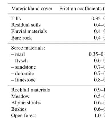
Table 2. Coefficients of friction for different materials and land cover (compiled from van Dijke and van Westen, 1990; Dorren and Seijmonsbergen, 2003; Wichmann, 2006).
Material/land cover Friction coefficients (µ)
Tills 0.35–0.5
Residual soils 0.4–0.5
Fluvial materials 0.4–0.5
Bare rock 0.4–0.9
Scree materials:
– marl 0.35–0.45
– flysch 0.6–0.7
– sandstone 0.7–0.8
– dolomite 0.7–0.8
– limestone 0.8–0.9
Rockfall materials 0.9–1.0
Meadow 0.5–0.6
Alpine shrubs 0.6–0.9
Bushes 0.6–0.7
Open forest 1.0–2.0
Dense forest >2.0
use they are not discussed in detail. A separate section pro-vides further information on scenario modeling. It must be noted that the parameter ranges provided for each process have to be considered as approximate values only and are thought to provide an initial guess. For example, Wichmann et al. (2008) have shown that for debris flow modeling the random walk and friction model parameters decrease with lower DTM resolutions.
4.1 Rockfall
Table 3.Model configuration for debris flow modeling on a regional scale and approximate parameter ranges (compiled from Zimmermann et al., 1997; Gamma, 2000; Wichmann and Becht, 2005; Wichmann, 2006).
Model component Model approach Parameter Value range
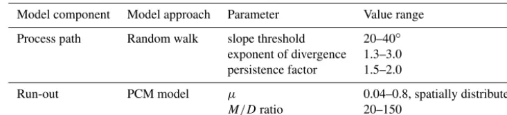
Process path Random walk slope threshold 20–40◦
exponent of divergence 1.3–3.0 persistence factor 1.5–2.0
Run-out PCM model µ 0.04–0.8, spatially distributed
M/Dratio 20–150
changes in direction already with the first impact on the talus slope. The exponent of divergence is comparatively high, too, in contrast to a rather small persistence factor which mimics the fact that rocks often change direction on impact.
The threshold of free fall used in the1-parameter friction modeldepends on the DTM resolution, but should conform with the slope threshold of theRandom Walkmodel. The en-ergy reduction on impact is usually about 75 %, as investi-gated by Broilli (1974). Although the dominating modes of motion of rockfalls are falling, bouncing and rolling, often a sliding motion is simulated for the sake of simplicity (e.g., van Dijke and van Westen, 1990; Meißl, 1998; Dorren and Seijmonsbergen, 2003; Wichmann and Becht, 2005). When the model is applied on a regional scale, the friction coeffi-cientµshould be provided, spatially distributed, as a raster data set. Table 2 shows sliding friction coefficients for dif-ferent materials and land cover. Spatially distributed friction coefficients are also very useful for scenario modeling, e.g., in order to determine the consequences of protection forest removal or reforestation.
The model configuration thus requires the following raster data sets as input: a DTM, a raster with release areas and a raster with spatially distributed friction coefficients. Model outputs, describing the derived process area, are raster data sets storing the transition frequencies, the encountered max-imum velocities and the stopping positions.
4.2 Debris flows
A typical model configuration for debris flow modeling on a regional scale is shown in Table 3. Again, theRandom Walk approach is used for path finding. The slope threshold is usu-ally set to angles slightly above the slope of the torrential fan. The exponent of divergence depends on the size of the simulated events. The larger the event, the higher the expo-nent. Its value also depends on the grain size and water con-tent, with lower values for flow slides and higher values for coarse-grained debris flows. The persistence factor is higher compared to rockfall as persistence is given in the case of debris flows.
Run-out distances are calculated on basis of the PCM model. The M/D drag ratio is usually calibrated once to match the highest observed velocities of a specific type of
debris flow. The friction parameterµis once again provided, spatially distributed, as a raster data set. Based on the ob-servation that the sliding friction coefficient tends towards lower values with increasing catchment area, attributed to a changing rheology with higher discharges along the process path, Gamma (2000) derived the following estimating func-tions from debris flows in Switzerland:
minimum run-out:µ=0.25·a−0.21,
likely run-out:µ=0.19·a−0.24,
maximum run-out:µ=0.13·a−0.25,
witha=catchment area (km2). Such data sets can be easily computed from a raster with stored catchment area (i.e., flow accumulation). Gamma (2000) and Wichmann and Becht (2005) additionally apply minimum (0.045) and maximum (0.3) thresholds in order to exclude extreme values. The model configuration thus requires a DTM, a raster with re-lease areas and a raster with spatially distributed friction coefficients as input. Model outputs, describing the derived process area, are again raster data sets storing transition fre-quencies, encountered maximum velocities and stopping po-sitions.
4.3 Avalanches
Table 4.Model configuration for avalanche modeling on a regional scale and approximate parameter ranges (compiled from Perla et al., 1980; Salm et al., 1990; Hegg, 1996; Heckmann, 2006; Schmidtner, 2012).
Model component Model approach Parameter Value range
Process path Random walk slope threshold 45–60◦
exponent of divergence 1.3–5.0 persistence factor 1.5–3.0
Run-out PCM model µ 0.1–0.5, spatially distributed
M/Dratio 20–1000, spatially distributed
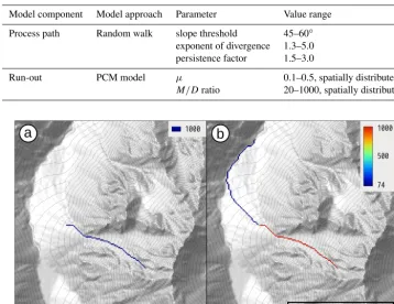
Figure 5.Sink filling:(a)the process stops in a sink;(b)the process overcomes the sink and stops in the next sink because no material is left.
4.4 Scenario modeling
Scenario modeling usually addresses topics such as process magnitude, the impact of protection forest or protection mea-sures. Different process magnitudes are usually modeled by using a different number of model iterations and/or friction coefficients. For example, different friction coefficients can be used to assess the relevance of protection forest by sim-ulating events with and without forest cover and to compare how the run-out distances increase (e.g., Wichmann, 2006; Proske and Bauer, 2016). Different friction coefficients have also been used to simulate different block sizes in rockfall modeling (e.g., Haas et al., 2012b). The influence of protec-tion measures can be analyzed by manipulating the DTM to include barriers or retention basins and to observe the impact on the extent of the processes area. Here, deposition model-ing is usually involved for sink fillmodel-ing. Deposition of material and sink filling are also required with high-resolution DTMs in order to fill up small depressions, to overcome obstacles or to simulate the break out of incised channels.
In order to demonstrate the approach for sink filling, a 10 m DTM has been modified to include a sink along the process path. For the sake of simplicity, the process path is modeled using theMaximum Slopeapproach with 1000 itera-tions and no friction and deposition models. Figure 5a shows
that the process stops at the end of the sink in the case that no material is provided. If 50 m3of material are provided, the process overcomes the sink and does not stop until the next sink is reached. This sink cannot be overcome because there is not enough material left.
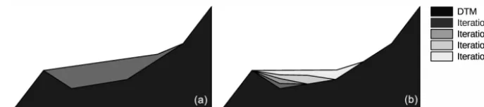
Figure 6 illustrates the sink-filling approach in detail. In the case that only a single iteration is calculated (Fig. 6a), all material provided is available in that iteration. The sink can thus be filled at once, preserving the slope specified with the minimum slope parameter (here 2.5◦). Figure 6b shows the successive filling of the sink when 10 model iterations are calculated and thus only 50/10=5 m3 of material are available per iteration.
Figure 7 shows the result of modeling two different mag-nitudes of debris flow events from five release areas on a hy-drologically sound 10 m DTM. The process path is modeled with theRandom Walkapproach (slope threshold=40◦,
-DTM
- Iteration 1
� Iteration 2 � Iteration 5 � Iteration 10
Figure 6.Longitudinal profile illustrating the sink-filling approach:(a)single model iteration,(b)10 model iterations.
The maximum velocities reached along the steeper parts of the process path are almost the same (16 m s−1for the large event, 15 m s−1 for the medium event), but the run-out dis-tances significantly increase with the lower friction valueµ
used for the large event. The stopping positions are well dis-tributed over the torrential fan because of the different pro-cess path lengths and slope profiles of the respective random walks. The number of stops per grid cell resembles the pat-tern of the transition frequencies.
Figure 8b and c show the modeling results of the large event from four release areas on a hydrologically sound 2.5 m DTM (same random walk and friction model settings as in the 10 m case above). At this DTM resolution the debris flow channels are sharply incised and the process path is forced to follow the channels in the case that no material deposition along the process path is simulated. Figure 8d–f show the result using 2750 m3of material in total (equally distributed over the release areas) and the deposition model approach min(slope;velocity) & on stop with the following parame-ter settings: initial deposition on stop=20 %, slope thresh-old=35◦, velocity threshold=12 m s−1, maximum deposi-tion along path=20 % and minimum path length=650 m. This parameter setting constrains the material deposition to the head of the torrential fan, successively filling up the in-cised channel and permitting the process to break out of the channel. In consequence, the process area covers the com-plete fan. Comparing the stopping positions (Fig. 8f) with the material deposition heights (Fig. 8e) it can be seen that although the deposition approach tries to deposit material while preserving a downward slope, new sinks are introduced in some cases because the available material per model iter-ation is not always enough to meet this requirement. Such sinks are then filled up in subsequent model iterations (see also Fig. 6b). It can also be seen that all of the provided ma-terial is already used up before the end of the process paths is reached.
5 Discussion and conclusion
The GPP model integrates several well known model ap-proaches, which are established in practice into a single GIS-based simulation framework. The framework is highly mod-ular, with components for process path, run-out length, sink filling and material deposition. The GPP model is a
concep-tual model, which provides the possibility to combine differ-ent modeling approaches and thus to model differdiffer-ent kinds of gravitational processes. The currently implemented mod-eling approaches are not entirely physically based, but build on empirical and basic principles to mimic typical macro-scopic characteristics of mass movements. Nowadays, sev-eral physically based numerical simulation models are avail-able (e.g., Iverson, 1997; Pudasaini and Hutter, 2007), which make it possible to simulate processes at a very high level of precision. However, these types of models require many (geotechnical) parameters such as rheological properties, co-hesion and substrate characteristics. The detailed information required and the real-world heterogeneity limit their appli-cability to small areas, usually to single events (Clerici and Perego, 2000; Guthrie et al., 2008).
Although some modeling approaches included in the GPP model are based on rather simple concepts, it is their com-plex interaction which permits the delineation of the extent of gravitational process areas. Reasonable results can be ob-tained with a minimum of input data and model parame-ters, recommending the framework especially for suscepti-bility mapping on regional scales. Recent additions such as the model components for sink filling and deposition model-ing make it also interestmodel-ing for scenario modelmodel-ing on various scales. Nevertheless, because of the limitations of the model it must be noted that this has to be done carefully on a lo-cal slo-cale. For example, different block sizes of rockfall can only be simulated indirectly by using different friction pa-rameters. Another limitation is the restriction of the process path routing to neighbor cells with equal or lower elevation, which makes the run-up of material on the opposite valley slope impossible. Like with every other simulation model it must be pointed out that it is a prerequisite to understand the functionality of the modeling approaches in detail before their application and the interpretation of the model results.
Figure 7. Medium (a–c) and large (d–f) debris flow events: (a) and (d) transition frequencies, (b) and (e) maximum velocities, and(c)and(f)stopping positions. For details see text.
Frameworks for the simulation of gravitational mass movements on a regional scale have been released by var-ious authors. For example, Horton et al. (2013) published the Flow-R (Flow path assessment of gravitational hazards at a Regional scale) model, which is a distributed empiri-cal model for regional susceptibility assessments of debris flows. It includes several flow-direction algorithms, but not all are relevant for gravitational mass movement modeling, and a random walk approach is missing. Flow-R also imple-ments two friction models: the approach of Perla et al. (1980) and the simplified friction-limited model (SFLM), which is based on the Fahrböschung principle (Heim, 1932). Flow-R is MATLAB-based and available free of charge for Win-dows and Linux, but its source code is not open. Mergili et al. (2015) developed the r.randomwalk model which offers built-in functions for model validation and has the ability to consider uncertainties. It is a multifunctional conceptual tool for backward and forward analyses of mass movement prop-agation and implemented as an add-on to GRASS GIS (but not officially included). It additionally requires the statistics software R (R Project for Statistical Computing). Currently the tool only works on UNIX systems with GRASS GIS 7.0 installed from source.
The GPP model is written in C++ and implemented in the “Geomorphology” tool library for the FOSS SAGA (Con-rad et al., 2015). It is thus completely integrated into a GIS environment which facilitates the preparation of input data and the analysis of the results. This avoids cumbersome data editing and data format conversions. Furthermore, the inte-gration of the model’s source code into the official SAGA source code repository will assure source code maintenance and easy application since the GPP model will be included in every SAGA binary release. It is running on Windows, Linux and Mac OS X.
Besides its purely scientific application, the GPP model also qualifies as kind of sandbox game because of its char-acteristics. Dynamic processes are reproduced by stochastic components and Monte Carlo simulation. Basically only a DTM and a map of release areas is required to get started. This allows its straightforward application in education. Ad-ditional information such as spatially distributed friction co-efficients derived from land cover maps are easily added for scenario modeling. This allows for example the visualization of the impact of protection forest decline on rockfall run-out length by simulating scenarios with and without forest cover through the application of different friction coefficients (see Table 2).
The GPP model is an attempt to bundle the development efforts put into several geomorphological process models within recent years into a single free and open-source ap-plication. It is the author’s opinion that making them avail-able in a new and free implementation, even extended by new components, is important for geomorphological- and natural-hazards-related research and education. The modular struc-ture of the framework and in particular of the source code facilitates the addition of further model approaches. The au-thor is looking forward to contributions such as the exten-sion of the framework through the addition of new modeling approaches or the implementation of accompanying SAGA tools, e.g., for automatic model parameter calibration based on observed events.
Code and data availability. The SAGA source code repository, in-cluding the GPP model, is hosted at https://sourceforge.net/projects/ saga-gis/ using a git repository. Read-only access is possible with-out log-in.
Alternatively, the source code and binaries can be downloaded directly from the files section at https://sourceforge.net/projects/ saga-gis/.
Appendix A
Table A1.The process path parameters of the GPP model.
Model Parameters Description
Maximum slope Iterations Number of model iterations from each start cell (–) Processing order Processing order of start cells; choice
Seed value Pseudo-random number generator initialization
Random walk Iterations Number of model iterations from each start cell (–) Processing order Processing order of start cells; choice
Seed value Pseudo-random number generator initialization Slope threshold Threshold below which lateral spreading is modeled (◦) Exponent Exponent controlling the amount of lateral spreading (–) Persistence factor Factor used as weight for the current flow direction (–)
Table A2.The run-out parameters of the GPP model.
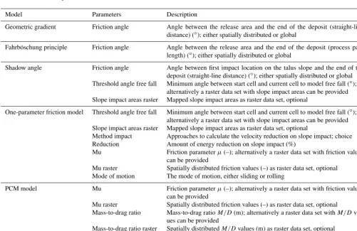
Model Parameters Description
Geometric gradient Friction angle Angle between the release area and the end of the deposit (straight-line distance) (◦); either spatially distributed or global
Fahrböschung principle Friction angle Angle between the release area and the end of the deposit (process path length) (◦); either spatially distributed or global
Shadow angle Friction angle Angle between first impact location on the talus slope and the end of the deposit (straight-line distance) (◦); either spatially distributed or global Threshold angle free fall Minimum angle between start cell and current cell to model free fall (◦);
alternatively a raster data set with slope impact areas can be provided Slope impact areas raster Mapped slope impact areas as raster data set, optional
One-parameter friction model Threshold angle free fall Minimum angle between start cell and current cell to model free fall (◦); alternatively a raster data set with slope impact areas can be provided Slope impact areas raster Mapped slope impact areas as raster data set, optional
Method impact Approaches to calculate the velocity reduction on slope impact; choice Reduction Amount of energy reduction on slope impact (%)
Mu Friction parameterµ(–); alternatively a raster data set with friction values can be provided
Mu raster Spatially distributed friction values (–) as raster data set, optional Mode of motion The mode of motion, either sliding or rolling
PCM model Mu Friction parameterµ(–); alternatively a raster data set with friction values
can be provided
Mu raster Spatially distributed friction values (–) as raster data set, optional
Mass-to-drag ratio Mass-to-drag ratioM/D(m); alternatively a raster data set withM/D val-ues can be provided
Table A3.The deposition parameters of the GPP model.
Model Parameters Description
Sink filling Minimum slope Minimum slope to preserve on sink filling (◦)
On stop Initial deposition on stop1 Percentage of available material initially deposited on stopping cell (%)
Slope & on stop Slope threshold2 Slope angle below which the deposition of material sets in (◦) Maximum deposition along Percentage of material which is deposited at most (%) process path1
Minimum path length1 Path length which has to be reached before material deposition is enabled (m)
Velocity & on stop Parameters denoted by1
Velocity threshold Velocity below which the deposition of material sets in (m s−1)
min(slope;velocity) & on stop Parameters denoted by1,2
1Also used by the models below.2Also used by themin(slope;velocity) & on stopmodel.
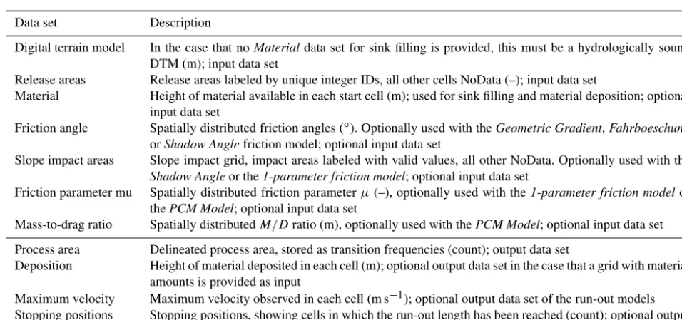
Table A4.The input and output data sets of the GPP model.
Data set Description
Digital terrain model In the case that noMaterialdata set for sink filling is provided, this must be a hydrologically sound DTM (m); input data set
Release areas Release areas labeled by unique integer IDs, all other cells NoData (–); input data set
Material Height of material available in each start cell (m); used for sink filling and material deposition; optional input data set
Friction angle Spatially distributed friction angles (◦). Optionally used with theGeometric Gradient,Fahrboeschung orShadow Anglefriction model; optional input data set
Slope impact areas Slope impact grid, impact areas labeled with valid values, all other NoData. Optionally used with the Shadow Angleor the1-parameter friction model; optional input data set
Friction parameter mu Spatially distributed friction parameterµ(–), optionally used with the1-parameter friction modelor thePCM Model; optional input data set
Mass-to-drag ratio Spatially distributedM/Dratio (m), optionally used with thePCM Model; optional input data set Process area Delineated process area, stored as transition frequencies (count); output data set
Deposition Height of material deposited in each cell (m); optional output data set in the case that a grid with material amounts is provided as input
Maximum velocity Maximum velocity observed in each cell (m s−1); optional output data set of the run-out models Stopping positions Stopping positions, showing cells in which the run-out length has been reached (count); optional output
The Supplement related to this article is available online at https://doi.org/10.5194/gmd-10-3309-2017-supplement.
Competing interests. The author declares that he has no conflict of interest.
Acknowledgements. The author would like to thank the Federal State of Vorarlberg for providing the remote sensing data sets, especially Peter Drexel (Landesvermessungsamt Feldkirch).
Edited by: Lutz Gross
Reviewed by: Gertraud Meißl and one anonymous referee
References
Aleotti, P. and Chowdhury, R.: Landslide hazard assessment: sum-mary review and new perspectives, B. Eng. Geol. Environ., 85, 21–44, 1999.
Broilli, L.: Ein Felssturz im Großversuch, Rock Mech., 3, 69–78, 1974.
Carrara, A., Cardinali, M., Detti, R., Guzzetti, F., Pasqui, V., and Reichenbach, P.: GIS Techniques and Statistical-Models in Eval-uating Landslide Hazard, Earth Surf. Proc. Land, 16, 427–445, 1991.
Clerici, A. and Perego, S.: Simulation of the Parma River blockage by the Corniglio landslide (Northern Italy), Geomorphology, 33, 1–23, 2000.
Conrad, O., Bechtel, B., Bock, M., Dietrich, H., Fischer, E., Gerlitz, L., Wehberg, J., Wichmann, V., and Böhner, J.: System for Auto-mated Geoscientific Analyses (SAGA) v. 2.1.4, Geosci. Model Dev., 8, 1991–2007, https://doi.org/10.5194/gmd-8-1991-2015, 2015.
Dorren, L. and Seijmonsbergen, A.: Comparison of three GIS-based models for predicting rockfall runout zones at a regional scale, Geomorphology, 56, 49–64, 2003.
Dorren, L. K. A.: A review of rockfall mechanics and modelling approaches, Progr. Phys. Geogr., 27, 69–87, 2003.
Fell, R., Corominas, J., Bonnard, C., Cascini, L., Leroi, E., and Sav-age, W. Z.: Guidelines for landslide susceptibility, hazard and risk zoning for land use planning, Eng. Geol., 102, 85–98, 2008. Freeman, T. G.: Calculating catchment area with divergent flow
based on a regular grid, Comput. Geosci., 17, 413–422, 1991. Gamma, P.: Großräumige Modellierung von Gebirgsgefahren
mit-tels rasterbasiertem Random Walk, in: Modellierung und Simu-lation räumlicher Systeme mit Geographischen Informationssys-temen, edited by: Mandl, P., Proceedings-Reihe der Informatik ’96, Klagenfurt, vol. 9, 93–105, 1996.
Gamma, P.: dfwalk – Ein Murgang-Simulationsprogramm zur Gefahrenzonierung, Geographica Bernensia, University of Bern, Switzerland, vol. G66, 14 pp., 2000.
Guthrie, R. H., Deadman, P. J., Cabrera, A. R., and Evans, S. G.: Exploring the magnitude–frequency distribution: a cellular au-tomata model for landslides, Landslides, 5, 151–159, 2008.
Haas, F., Heckmann, T., Hilger, L., and Becht, M.: Quantifica-tion and Modelling of Debris Flows in the Proglacial Area of the Gepatschferner/Austria using Ground-based LIDAR, IAHS-AISH P., 356, 293–302, 2012a.
Haas, F., Heckmann, T., Wichmann, V., and Becht, M.: Runout anal-ysis of a large rockfall in the Dolomites/Italian Alps using LI-DAR derived particle sizes and shapes, Earth Surf. Proc. Land., 37, 1444–1455, 2012b.
Heckmann, T.: Untersuchungen zum Sedimenttransport durch Grundlawinen in zwei Einzugsgebieten der Nördlichen Kalka-lpen: Quantifizierung, Analyse und Ansätze zur Modellierung der geomorphologischen Aktivität, Eichstätt. Geogr. Arb., vol. 14, 340 pp., 2006.
Heckmann, T. and Schwanghart, W.: Geomorphic coupling and sediment connectivity in an alpine catchment – Exploring sedi-ment cascades using graph theory, Geomorphology, 182, 89–103, 2013.
Heckmann, T., Hilger, L., Vehling, L., and Becht, M.: Integrat-ing field measurements, a geomorphological map and stochastic modelling to estimate the spatially distributed rockfall sediment budget of the Upper Kaunertal, Austrian Central Alps, Geomor-phology, 260, 16–31, 2016.
Hegg, C.: Zur Erfassung und Modellierung von gefährlichen Prozessen in steilen Wildbacheinzugsgebieten, Geographica Bernensia, University of Bern, Switzerland, vol. G52, 197 pp., 1996.
Heim, A.: Bergsturz und Menschenleben, Beiblatt zur Viertel-jahrschrift der Naturforschenden Gesellschaft in Zürich, 77, 218 pp., 1932.
Heinimann, H. R., Hollenstein, K., Kienholz, H., Krummenacher, B., and Mani, P.: Methoden zur Analyse und Bewertung von Naturgefahren, in: Umwelt-Materialien Naturgefahren, Bunde-samt für Umwelt, vol. 85, p. 248, 1998.
Horton, P., Jaboyedoff, M., Rudaz, B., and Zimmermann, M.: Flow-R, a model for susceptibility mapping of debris flows and other gravitational hazards at a regional scale, Nat. Hazards Earth Syst. Sci., 13, 869–885, https://doi.org/10.5194/nhess-13-869-2013, 2013.
Hu, K., Li, P., You, Y., and Su, F.: A Hydrologically Based Model for Delineating Hazard Zones in the Valleys of De-bris Flow Basins, Nat. Hazards Earth Syst. Sci. Discuss., https://doi.org/10.5194/nhess-2016-13, 2016.
Hungr, O. and Evans, S. G.: Engineering evaluation of fragmen-tal rockfall hazards, in: Landslides, edited by: Bonnard, C., Pro-ceedings of the 5th International Symposium on Landslides, Lau-sanne, Switzerland, 10–15 July l988, 685–690, 1988.
Iverson, R. M.: The physics of debris flows, Rev. Geophys., 35, 245–296, 1997.
Jenson, S. K. and Domingue, J. O.: Extracting topographic structure from digital elevation data for Geographic Information System analysis, Photogramm. Eng. Rem. S., 54, 1593–1600, 1988. Kirkby, M. J. and Statham, I.: Surface stone movement and scree
formation, J. Geol., 83, 349–362, 1975.
Körner, H. J.: Reichweite und Geschwindigkeit von Bergstürzen und Fließschneelawinen, Rock Mech., 8, 225–256, 1976. Körner, H. J.: The energy-line method in the mechanics of
Lied, K. and Bakkehøi, S.: Empirical calculations of snow avalanche run-out distance based on topographic parameters, J. Glaciol., 26, 165–177, 1980.
Meißl, G.: Modellierung der Reichweite von Felsstürzen, Inns-brucker Geographische Studien, Innsbruck, vol. 28, 249 pp., 1998.
Mergili, M., Fellin, W., Moreiras, S. M., and Stötter, J.: Simulation of debris flows in the Central Andes based on Open Source GIS: possibilities, limitations, and parameter sensitivity, Nat. Hazards, 61, 1051–1081, 2012.
Mergili, M., Krenn, J., and Chu, H.-J.: r.randomwalk v1, a multi-functional conceptual tool for mass movement routing, Geosci. Model Dev., 8, 4027–4043, https://doi.org/10.5194/gmd-8-4027-2015, 2015.
Nohguchi, Y.: Three-Dimensional Equations for Mass Centre Mo-tion of anAvalanche of Arbitrary ConfiguraMo-tion, Ann. Glaciol., 13, 215–217, 1989.
O’Callaghan, J. and Mark, D.: The extraction of drainage networks from digital elevation data, Comput. Vision Graph., 28, 323–344, 1984.
Perla, R., Cheng, T. T., and McClung, D. M.: A two-parameter model of snow-avalanche motion, J. Glaciol., 26, 197–207, 1980. Proske, H. and Bauer: Rockfall Susceptibility Maps in Styria con-sidering the protective effect of forest, in: INTERPRAEVENT 2016, edited by: Koboltschnig, G., Conference Proceedings, 592–600, 2016.
Pudasaini, S. P. and Hutter, K.: Avalanche Dynamics: Dynamics of rapid flows of dense granular avalanches, Springer, Berlin, Ger-many, 2007.
Rickenmann, D.: Debris flows 1987 in Switzerland: modelling and fluvial sediment transport, IAHS-AISH P., 194, 371–378, 1990. Salm, B., Burkard, A., and Gubler, H.: Berechnung von
Fließch-neelawinen. Eine Anleitung für Praktiker mit Beispielen, Mit-teilungen des Eidgenössischen Instituts für Schnee- und Law-inenforschung, Davos, p. 37, 1990.
Scheidegger, A. E.: Physical Aspects of Natural Catastrophes, Else-vier, Amsterdam, 1975.
Schmidtner, K.: Modellierung ausgewählter Lawinenereignisse in Südtirol, Ein Beitrag zur Optimierung der modellsteuernden Pa-rameter und zur Entwicklung von Möglichkeiten der wechsel-seitigen Ergänzung der Modelle: RAMMS, ELBA+, Aval-Walk, Analytisches Voellmy-Salm, 144 pp., 2012.
Takahashi, T., Nakagawa, H., Harada, T., and Yamashiki, Y.: Rout-ing debris flows with particle segregation, J. Hydraul. Eng., 118, 1490–1507, 1992.
van Dijke, J. J. and van Westen, C. J.: Rockfall Hazard: a Geomor-phologic Application of Neighbourhood Analysis with ILWIS, ITC Journal 1990, 1, 40–44, 1990.
van Westen, C. J., van Asch, T. W. J., and Soeters, R.: Landslide hazard and risk zonation – why is it so difficult?, B. Eng. Geol. Environ., 65, 167–184, 2006.
Voellmy, A.: Über die Zerstörungskraft von Lawinen, Schweiz-erische Bauzeitung, 73, 159–165, 212–217, 246–249, 280–285, 1955.
Wichmann, V.: Modellierung geomorphologischer Prozesse in einem alpinen Einzugsgebiet – Abgrenzung und Klassifizierung der Wirkungsräume von Sturzprozessen und Muren mit einem GIS, Eichstätt. Geogr. Arb., vol. 15, 231 pp., 2006.
Wichmann, V. and Becht, M.: Spatial modelling of debris flows in an alpine drainage basin, IAHS-AISH P., 288, 370–376, 2004. Wichmann, V. and Becht, M.: Modelling Of Geomorphic Processes
In An Alpine Catchment, in: Geodynamics, edited by: Atkinson, P. M., Foody, G. M., Darby, S. E., and Wu, F., CRC Press, Boca Raton, 151–167, 2005.
Wichmann, V. and Becht, M.: Rockfall modelling: methods and model application in an alpine basin (Reintal, Germany), in: SAGA – Analysis and Modelling Applications, edited by: Böh-ner, J., McCloy, K. R., and Strobl, J., Göttinger Geographische Abhandlungen, no. 115, 105–116, 2006.
Wichmann, V., Rutzinger, M., and Vetter, M.: Digital Terrain Model Generation from airborne Laser Scanning Point Data and the Ef-fect of grid-cell size on the Simulation Results of a Debris Flow Model, in: SAGA – Seconds Out, edited by: Böhner, J., Blaschke, T., and Montanarella, L., Hamburger Beiträge zur Physischen Geographie und Landschaftsökologie, Univ. Hamburg, Inst. für Geographie, no. 19, 103–113, 2008.
Wichmann, V., Heckmann, T., Haas, F., and Becht, M.: A new mod-elling approach to delineate the spatial extent of alpine sediment cascades, Geomorphology, 111, 70–78, 2009.