Cost Effective Operating Strategy for Unit Commitment and Economic Dispatch of Thermal Power Plants with Cubic Cost Functions Using TLBO Algorithm

http://dx.doi.org/10.4236/jpee.2015.36003

Cost Effective Operating Strategy for Unit

Commitment and Economic Dispatch of

Thermal Power Plants with Cubic Cost

Functions Using TLBO Algorithm

E. B. Elanchezhian, S. Subramanian, S. Ganesan

Department of Electrical Engineering, Annamalai University, Chidambaram, India Email: [email protected]

Received 11 May 2015; accepted 16 June 2015; published 19 June 2015

Copyright © 2015 by authors and Scientific Research Publishing Inc.

This work is licensed under the Creative Commons Attribution International License (CC BY).

http://creativecommons.org/licenses/by/4.0/

Abstract

This paper deals with a Unit Commitment (UC) problem of a power plant aimed to find the optimal scheduling of the generating units involving cubic cost functions. The problem has non convex ge-nerator characteristics, which makes it very hard to handle the corresponding mathematical models. However, Teaching Learning Based Optimization (TLBO) has reached a high efficiency, in terms of solution accuracy and computing time for such non convex problems. Hence, TLBO is applied for scheduling of generators with higher order cost characteristics, and turns out to be computation-ally solvable. In particular, we represent a model that takes into account the accurate higher order generator cost functions along with ramp limits, and turns to be more general and efficient than those available in the literature. The behavior of the model is analyzed through proposed tech-nique on modified IEEE-24 bus system.

Keywords

Cubic Cost Functions, Ramp Rate, Teaching Learning Based Optimization, Unit Commitment

1. Introduction

preparation of “real time” control of an electrical network. One of these processing functions is the determina-tion of thermal Unit Commitment (UC). The UC problem is a large-scale, non-convex, non-linear, and mixed integer optimization problem. The optimal solution of the problem can be obtained by complete enumeration, which is prohibitive in practice owing to its excessive computational resource requirements. So, attempts are being continuously made to solve this problem by reliable iterative and heuristic methods.

A bibliographical survey on UC reveals that a good amount of numerical optimization techniques [1]-[4] and meta-heuristic [5]-[13] methods have been applied to achieve efficient and near optimal solutions. Traditionally to solve the UC effectively, conventional techniques need the incremental fuel cost curves to be featured of mo-notonically increasing and continuous. But practically, the generating units actually have non-monotonic incre-mental fuel cost curves. For simplicity and easy solving purposes, the input-output characteristics of thermal generators are usually approximated by quadratic functions or piecewise linear functions [1]-[13]. However, many approaches have been addressed that the Economic Dispatch (ED) solution accuracy can be improved or the exact cost can be obtained with higher order functions or Cubic Cost Functions (CCF) [14]-[17]. Earlier pa-pers in the literature have not considered the third order cost functions because they focus on their algorithms and lost the accuracy by approximating the realistic cost curve. In our previous work, we proposed an economic dispatch model using CCF [17]. Even though the UC research is solved for past years, less work is carried out for UC with Cubic Cost Functions (UC-CCF).

The evolutionary and population based techniques in the literature survey are probabilistic techniques and necessitate some common controlling parameters like population size, number of generations and elite size. Moreover, the algorithms also require finding of some of their own control parameters. Genetic Algorithm (GA) needs crossover rate and mutation rate, Particle Swarm Optimization (PSO) has its own parameters like inertia weight, and social and cognitive parameters. The global solution of any function is only achieved with the prop-er tuning of these algorithm-specific parametprop-ers. Impropprop-er tuning may lead to local optimal solution or increase in convergence time.

In this paper, a recently developed heuristic algorithm named teaching learning based optimization (TLBO) algorithm based on the effect of the influence of a teacher on the output of learners in a class, introduced by Rao

et al. [18], is utilized for the solution of UC problem. This TLBO algorithm has been implemented in various

problem domains of engineering and technology. Most recently, it has been utilized in solving a few areas in power system [17] [19]-[21]. Unlike other population based techniques, TLBO requires only determination of common controlling parameters like population size and number of generations for its functionality. In the present work, TLBO based UC (TLBO-UC) with CCF (TLBO-UC-CCF) is carried on 26-unit test system con-sidering ramp rate constraints for a time horizon of 24 hours to prove the scalability of the algorithm.

2. Unit Commitment Problem Formulation

Mathematically, the unit commitment problem can be formulated as a mixed integer non-linear problem. The objective function and constraints are formulated as given below.

2.1. Objective Function

The objective function of UC problem is the minimization of the total cost (FTuc) (Equation (1)) which is the

sum of the fuel cost (F) and the start up cost (SUC) of individual units (N) for the given period (T) subject to various constraints. Mathematically, the UC problem model can be formulated as

( )

(

)

(

)

1 1

Minimize _Tuc T N _{it i i i} 1 _{i t} t i

F U F P t SUC U −

= =

 

=

∑∑

where FTuc is the total operating cost in $, Fi (Pi (t)) is the fuel cost of unit i at hour t, Pi (t) is the output power of ith _{unit at hour t, U}

itis the on/off status of ith unit at hour t.

The major component of the operating cost, for thermal units, is the power production cost of the committed units that is modelled as third order cubic function as shown in Equation (2)

( )

( )

_{$ h}

i i i i i i i i i

F P

= +

a b P c p d P

+

+

2.2. Constraints

2.2.1 System Power Balance

( )

( )

1

, 1,2, , N

i i d

i= U P t P t t T

= =

∑

where Pd(t) is the power demand at tth interval.

2.2.2. Spinning Reserve Constraints

The sum of the maximum power generating capacities of all the committed units at a time instant should be at least equal to the sum of the known power demand and minimum spinning reserve requirement at that time in-stant, i.e.

(max)

( )

1 , 1,2, ,

N

it i d t

i= U P P t R t T

≥ + =

∑

where Pi (max) is the known maximum power that can be generated by unit i at any time instant and Rt is the

minimum spinning reserve requirement at time t.

2.2.3. Generation Limit Constraints

( )min

( )

i i i

P ≤P t ≤P U =

( )

i it

P t = U = (5) where Pi (min) and Pi (max) represents the minimum and maximum generation limits of thermal units.

2.2.4. Unit Minimum up/down Time Constraints

( )1 ( )1 ( ) 0

on on

i

i t i t i t

X − T U − U

 −  ∗ − ≥

    (6)

( )1 ( ) ( )1 0

off off i

i t i t i t

X − T U U −

 ₋  _{∗ −} _≥

    (7) where on_{( )}

i t

X and off_{( )} i t

X is the time duration for which unit i has been on and off respectively at hour t.

2.2.5. Ramp Rate Limits

( )

(

)

i i i

P t −P t− ≤UR As generation increases (8)

(

)

( )

i i i

P t− −P t ≤DR As generation decreases (9)

where UR and DR represents the generator ramp up and ramp down limits

3. Teaching Learning Based Optimization

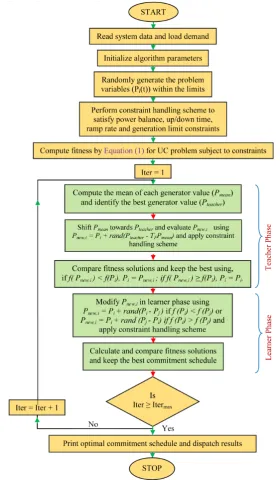
The steps involved in the search procedure of the TLBO algorithm for the proposed UC-CCF problem is illu-strated by flowchart inFigure 1 and are summarized as follows.

Initialization of TLBO-UC-CCF problem

Step 1: Define the UC-CCF optimization problem as minimization problem.

Step 2: Population size (Ps), number of design variables (Nd) which represents number of generating units, minimum up/down time, initial status, maximum and minimum generation limits (limits of design variables) and stopping criteria (maximum number of iterations) are defined in this step.

Teacher phase

Step 3: Evaluate the difference between existing mean and best mean result by utilizing Teaching factor (Tf). Learner phase

Step 4: Update the learner’s generation solution with the help of teacher’s generation.

Step 5: Update the learner’s generating solution by utilizing the generating solution of some other learner.

Termination criteria

Step 6: Repeat the procedure from Step 2 to 5 till the maximum number of iterations is met.

Constraint Handling Techniques

A key factor in the application of heuristic algorithms to UC problem is how the algorithm handles the con-straints relating to the problem. In the proposed solution method, the concon-straints of the UC are implemented us-ing a combination of preservation and penalty function methods. The generatus-ing capacity limits and ramp up/down rate constraints are also handled by the preservation method. The production of the initial population and in the two phases of TLBO, the output of all committed units minus the reference unit are chosen arbitrary within their respective generating capacity limits, whereas the output of the reference unit is constrained by the system power balance constraint. So, for the dispatchable units other than reference unit, the generating capacity limit constraint is automatically satisfied in both initial population and two phases of TLBO. Therefore, the vi-olation of the capacity limit constraint should be only considered as the penalty term for the reference unit. The minimum up-time/down-time duration constraints of the UC problem are checked for each unit over the sche-duling horizon in each interval. If there is any violation in the minimum up or minimum down time constraint then repair mechanism [11] is used to overcome the violation.

4. Numerical Simulation Results and Discussions

In this section, the numerical results aimed at showing the efficiency and the effectiveness of the proposed ap-proach is presented. The proposed TLBO-UC method is tested on modified IEEE-24 bus system having 26 units over a 24-hour scheduling horizon. In order to avoid misleading results due to the stochastic nature of the TLBO, 100 runs were averaged with each run starting with random initial populations. The performance of the proposed problem is implemented using MATLAB-7.9 and realized in 2.40 GHz, i3 processor with 4 GB RAM. The ob-tained results are compared with other methods in the literature.

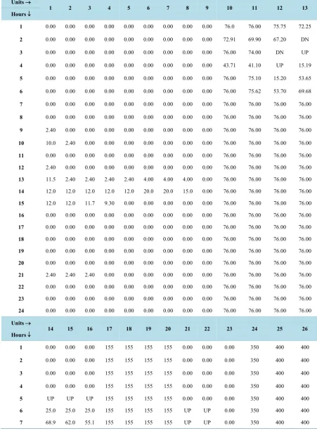
This test system consists of 26 units involving cubic cost equations. System particulars involving system data, load demand, ramp rate and capacity limits of the aforementioned units are obtained from literature [2] [3] [14] [15]. In order to determine the best parameters of the proposed TLBO, a number of simulations are carried out. After a number of careful experimentation, following optimal values of TLBO-UC parameters have finally been settled and most appropriate to adopt: Population size (Ps) = 30 and Number of iterations = 100. These parame-ters are obtained from fine tuning process which is problem dependant task. Simulations are carried out for a 24 hour horizon. The generation cost, % reserve and start-up cost for 24 hour horizon is shown inTable 1. The op-timal commitment schedule and generation output derived by the proposed algorithm considering the ramp rate and cubic cost equation is shown inTable 2 for 24 hour horizon.

In this combination for unit scheduling and generation output, the total generation cost obtained by the pro-posed approach is $795488.869.Table 3 shows the comparison of the total generation cost and execution time achieved by TLBO method with the popular methods, e.g. Piecewise Linear Iterative (PLI) [15] and Dynamic Programming-Sequential and Truncated Combination (DP-STC) [15]. The corresponding generation cost using the PLI and DP-STC is $795698.33 and $795489.09 respectively. The total operation cost considering start-up cost obtained by TLBO is $800158.869.

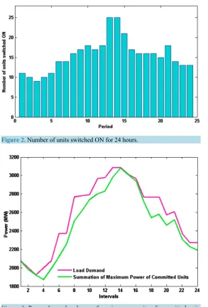
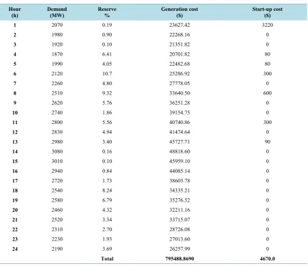
For the 26 unit system, the number of units committed for the entire scheduling period is shown inFigure 2. Figure 3 illustrates variation of load demand and the summation of the maximum capacity of the committed units for each hour in the entire time horizon.Figure 4 exemplify the generating units ON/OFF status of the 26 unit system for 24 hour horizon. Execution time complexity of each optimization method is very important for its application to real systems.Table 3 shows the execution time of 0.32 seconds which is less than the other methods in literature. The performance analysis of the test system involving CCF as considered by the authors of the present work being totally a new one, no comparison could be done with regard to the performance analy-sis results. The best, average and worst fuel costs among the 100 runs of algorithm satisfying the system con-straints are listed inTable 4.

Figure 2.Number of units switched ON for 24 hours.

Figure 3. Power demand and sum of maximum capacity of committed units for 24 hours.

values of the standard deviation confirm the capability and reliability of the TLBO to find the best compromise solution. The success rate is defined as (RunSuccess/RunTot) x 100, where RunSuccess is the number of successful

ex-periments which converge to the best solution within the range and RunTot is the total number of runs performed. Results of the success rate for 26-unit with cubic cost functions is 63% and is listed in Table 4 which demon-strates that TLBO has satisfactory success rate. From the results, it is clear that the proposed method is robust and it is applicable to practical systems.

Figure 4. Units ON/OFF representation of 26 unit test system for 24 hours.

Table 1.Operation costs and available reserve for 24 hours. Hour

(h) Demand (MW) Reserve % Generation cost ($) Start-up cost ($)

1 2070 0.19 23627.42 3220

2 1980 0.90 22268.16 0

3 1920 0.10 21351.82 0

4 1870 6.41 20701.82 80

5 1990 4.05 22482.68 80

6 2120 10.7 25286.92 300

7 2260 4.80 27778.05 0

8 2510 9.32 33640.50 600

9 2620 5.76 36251.28 0

10 2740 1.86 39154.75 0

11 2800 5.56 40740.86 300

12 2830 4.94 41474.64 0

13 2980 3.40 45727.71 90

14 3080 0.16 48818.60 0

15 3010 0.10 45959.10 0

16 2940 0.84 44085.14 0

17 2720 1.73 38603.78 0

18 2540 8.24 34335.21 0

19 2580 6.79 35276.52 0

20 2460 4.32 32211.16 0

21 2520 3.34 33715.07 0

22 2310 2.70 28726.08 0

23 2230 1.93 27013.60 0

24 2190 3.69 26257.99 0

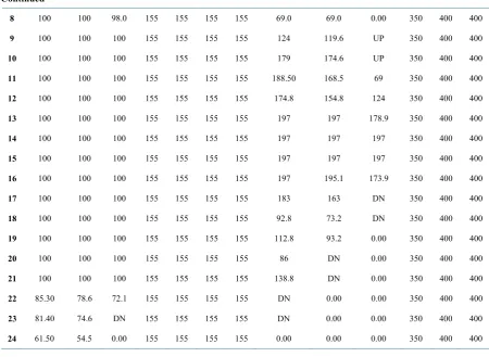
Table 2. Optimal scheduling of modified IEEE-24 bus system.

Units →

1 2 3 4 5 6 7 8 9 10 11 12 13

Hours ↓

1 0.00 0.00 0.00 0.00 0.00 0.00 0.00 0.00 0.00 76.0 76.00 75.75 72.25

2 0.00 0.00 0.00 0.00 0.00 0.00 0.00 0.00 0.00 72.91 69.90 67.20 DN

3 0.00 0.00 0.00 0.00 0.00 0.00 0.00 0.00 0.00 76.00 74.00 DN UP

4 0.00 0.00 0.00 0.00 0.00 0.00 0.00 0.00 0.00 43.71 41.10 UP 15.19

5 0.00 0.00 0.00 0.00 0.00 0.00 0.00 0.00 0.00 76.00 75.10 15.20 53.65

6 0.00 0.00 0.00 0.00 0.00 0.00 0.00 0.00 0.00 76.00 75.62 53.70 69.68

7 0.00 0.00 0.00 0.00 0.00 0.00 0.00 0.00 0.00 76.00 76.00 76.00 76.00

8 0.00 0.00 0.00 0.00 0.00 0.00 0.00 0.00 0.00 76.00 76.00 76.00 76.00

9 2.40 0.00 0.00 0.00 0.00 0.00 0.00 0.00 0.00 76.00 76.00 76.00 76.00

10 10.0 2.40 0.00 0.00 0.00 0.00 0.00 0.00 0.00 76.00 76.00 76.00 76.00

11 0.00 0.00 0.00 0.00 0.00 0.00 0.00 0.00 0.00 76.00 76.00 76.00 76.00

12 2.40 0.00 0.00 0.00 0.00 0.00 0.00 0.00 0.00 76.00 76.00 76.00 76.00

13 11.5 2.40 2.40 2.40 2.40 4.00 4.00 4.00 0.00 76.00 76.00 76.00 76.00

14 12.0 12.0 12.0 12.0 12.0 20.0 20.0 15.0 0.00 76.00 76.00 76.00 76.00

15 12.0 12.0 11.7 9.30 0.00 0.00 0.00 0.00 0.00 76.00 76.00 76.00 76.00

16 0.00 0.00 0.00 0.00 0.00 0.00 0.00 0.00 0.00 76.00 76.00 76.00 76.00

17 0.00 0.00 0.00 0.00 0.00 0.00 0.00 0.00 0.00 76.00 76.00 76.00 76.00

18 0.00 0.00 0.00 0.00 0.00 0.00 0.00 0.00 0.00 76.00 76.00 76.00 76.00

19 0.00 0.00 0.00 0.00 0.00 0.00 0.00 0.00 0.00 76.00 76.00 76.00 76.00

20 0.00 0.00 0.00 0.00 0.00 0.00 0.00 0.00 0.00 76.00 76.00 76.00 76.00

21 2.40 2.40 2.40 0.00 0.00 0.00 0.00 0.00 0.00 76.00 76.00 76.00 76.00

22 0.00 0.00 0.00 0.00 0.00 0.00 0.00 0.00 0.00 76.00 76.00 76.00 76.00

23 0.00 0.00 0.00 0.00 0.00 0.00 0.00 0.00 0.00 76.00 76.00 76.00 76.00

24 0.00 0.00 0.00 0.00 0.00 0.00 0.00 0.00 0.00 76.00 76.00 76.00 76.00

Units →

14 15 16 17 18 19 20 21 22 23 24 25 26

Hours ↓

1 0.00 0.00 0.00 155 155 155 155 0.00 0.00 0.00 350 400 400

2 0.00 0.00 0.00 155 155 155 155 0.00 0.00 0.00 350 400 400

3 0.00 0.00 0.00 155 155 155 155 0.00 0.00 0.00 350 400 400

4 0.00 0.00 0.00 155 155 155 155 0.00 0.00 0.00 350 400 400

5 UP UP UP 155 155 155 155 0.00 0.00 0.00 350 400 400

6 25.0 25.0 25.0 155 155 155 155 UP UP 0.00 350 400 400

Continued

8 100 100 98.0 155 155 155 155 69.0 69.0 0.00 350 400 400

9 100 100 100 155 155 155 155 124 119.6 UP 350 400 400

10 100 100 100 155 155 155 155 179 174.6 UP 350 400 400

11 100 100 100 155 155 155 155 188.50 168.5 69 350 400 400

12 100 100 100 155 155 155 155 174.8 154.8 124 350 400 400

13 100 100 100 155 155 155 155 197 197 178.9 350 400 400

14 100 100 100 155 155 155 155 197 197 197 350 400 400

15 100 100 100 155 155 155 155 197 197 197 350 400 400

16 100 100 100 155 155 155 155 197 195.1 173.9 350 400 400

17 100 100 100 155 155 155 155 183 163 DN 350 400 400

18 100 100 100 155 155 155 155 92.8 73.2 DN 350 400 400

19 100 100 100 155 155 155 155 112.8 93.2 0.00 350 400 400

20 100 100 100 155 155 155 155 86 DN 0.00 350 400 400

21 100 100 100 155 155 155 155 138.8 DN 0.00 350 400 400

22 85.30 78.6 72.1 155 155 155 155 DN 0.00 0.00 350 400 400

23 81.40 74.6 DN 155 155 155 155 DN 0.00 0.00 350 400 400

24 61.50 54.5 0.00 155 155 155 155 0.00 0.00 0.00 350 400 400

Table 3. Comparison of best results obtained by different methods.

Method Total start-up _{cost ($)} generation Total cost ($)

Total operation

cost ($)

Execution time (s)

PLI - 795698.3300 - 0.33

DP-STC - 795489.0900 - 0.34

TLBO 4670 795488.8690 800158.869 0.32

Table 4. Performance analysis of best feasible solution for 26 unit test system by TLBO.

Test system 26-unit _system

Population size 30

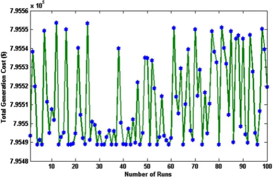
Best cost ($) 795488.8690

Average cost ($) 795509.9318

Worst cost ($) 795553.5564

Standard deviation 22.515

Success rate

795,488 ($) - 795,510 ($) 63%

Figure 5. Distribution of the best generation cost of each simulation run for 24 hours.

5. Conclusions

In this paper, a nature inspired TLBO technique has been proposed for solving unit commitment problem with ramp constraints on the thermal generating units involving cubic cost functions. The keys of the effectiveness of the approach are the efficient algorithm for ED problems with cubic cost equations recently proposed that ex-actly solves the UC problem involving non-convex higher order cost functions without any form of approxima-tion. The sophisticated heuristics for producing a ramp feasible and demand feasible solution is developed. Solving ramp constrained UC problem turns out to be efficient with high provable accuracy on large scale realistic in-stances in reasonable computational time. The proposed TLBO-UC-CCF method remarkably reduces the gener-ation cost and computgener-ation time, and yields more accurate genergener-ation scheduling, which shows its adaptability to any higher order generation cost functions.

Incorporating reserve constraints in the UC problem is usually difficult; indeed, they are often used in litera-ture. However, extending our approach to reserve constrained UC with higher order cost functions is not straightforward, and it will be the subject of a future work.

Acknowledgements

The authors gratefully acknowledge the authorities of Annamalai University, Annamalai Nagar, Tamilnadu, In-dia for the facilities provided to carry out this research work.

References

[1] Wood, A.J. and Woolenberg, B.F. (1996) Power Generation, Operation and Control. Wiley, New York.

[2] Tong, S.K., Shahidehpour, S.M. and Ouyang, Z. (1991) A Heuristic Short-Term Unit Commitment. IEEE Transactions on Power Systems, 6, 1210-1216. http://dx.doi.org/10.1109/59.119268

[3] Wang, C. and Shahidehpour, S.M. (1993) Effects of Ramp Rate Limits on Unit Commitment and Economic Dispatch.

IEEE Transactions on Power Systems, 8, 1341-1350. http://dx.doi.org/10.1109/59.260859

[4] Wang, S.J., Shahidehpour, S.M., Kirschen, D.S., Mokhtari, S. and Irisarri, G.D. (1995) Short Term Generation Sche-duling with Transmission and Environmental Constraints Using an Augmented Lagrangian Relaxation. IEEE Transac-tions on Power Systems, 10, 1294-1301. http://dx.doi.org/10.1109/59.466524

[5] Dudek, G. (2004) Unit Commitment by Genetic Algorithm with Specialized Search Operators. Electric Power Systems Research, 72, 299-308. http://dx.doi.org/10.1016/j.epsr.2004.04.014

[6] Wang, L.F. and Singh, C. (2009) Unit Commitment Considering Generator Outages through a Mixed-Integer Particle Swarm Optimization. Applied Soft Computing, 9, 947-953. http://dx.doi.org/10.1016/j.asoc.2008.11.010

Problem. IEEE Transactions on Power Systems, 24, 1478-1488. http://dx.doi.org/10.1109/TPWRS.2009.2021216 [8] Ebrahimi, J., Hosseinian, S.H. and Gharehpetian, G.B. (2011) Unit Commitment Problem Solution using Shuffled Frog

Leaping Algorithm. IEEE Transactions on Power Systems, 26, 573-581. http://dx.doi.org/10.1109/TPWRS.2010.2052639

[9] Abookazemi, K., Ahmad, H., Tavakolpour, A. and Hassan, M.Y. (2011) Unit Commitment Solution Using an Opti-mized Genetic System. International Journal of Electrical Power & Energy Systems, 33, 969-975.

http://dx.doi.org/10.1016/j.ijepes.2011.01.009

[10] Vaisakh, K. and Srinivas, L.R. (2011) Evolving Ant Colony Optimization Based Unit Commitment. Applied Soft Computing, 11, 2863-2870. http://dx.doi.org/10.1016/j.asoc.2010.11.019

[11] Chandrasekaran, K., Hemamalini, S., Simon, S.P. and Padhy, N.P. (2012) Thermal Unit Commitment Using Binary/ Real Coded Artificial Bee Colony Algorithm. Electric Power Systems Research, 84, 109-119.

http://dx.doi.org/10.1016/j.epsr.2011.09.022

[12] Datta, D. and Dutta, S. (2012) A Binary-Real-Coded Differential Evolution for Unit Commitment Problem. Interna-tional Journal of Electrical Power & Energy Systems, 42, 517-524. http://dx.doi.org/10.1016/j.ijepes.2012.04.048 [13] Roy, P.K. and Sarkar, R. (2014) Solution of Unit Commitment Problem Using Quasi-Oppositional Teaching Learning

Based Algorithm. International Journal of Electrical Power & Energy Systems, 60, 96-106. http://dx.doi.org/10.1016/j.ijepes.2014.02.008

[14] Moon, Y.H., Park, J.K., Kook, H.J. and Lee, Y.H. (2001) A New Economic Dispatch Algorithm Considering Any Higher Order Generation Cost Functions. International Journal of Electrical Power & Energy Systems, 23, 113-118. http://dx.doi.org/10.1016/S0142-0615(00)00043-0

[15] Lin, W.-M., Gow, H.-J. and Tsay, M.-T. (2007) A Partition Approach Algorithm for Non-Convex Economic Dispatch.

International Journal of Electrical Power & Energy Systems, 29, 432-438. http://dx.doi.org/10.1016/j.ijepes.2006.11.002

[16] Saber, A.Y., Chakraborthy, S., Abdur Razzak, S.M. and Senjyu, T. (2009) Optimization of Economic Load Dispatch of Higher Order General Cost Polynomials and Its Sensitivity Using Modified Particle Swarm Optimization. Electric Power Systems Research, 79, 98-106. http://dx.doi.org/10.1016/j.epsr.2008.05.017

[17] Elanchezhian, E.B., Subramanian, S. and Ganesan, S. (2014) Economic Power Dispatch with Cubic Cost Models Us-ing TeachUs-ing LearnUs-ing Algorithm. IET Generation, Transmission & Distribution, 8, 1187-1202.

http://dx.doi.org/10.1049/iet-gtd.2013.0603

[18] Rao, R.V., Savsani, V.J. and Vakharia, D.P. (2012) Teaching-Learning-Based Optimization: An Optimization Method for Continuous Non-Linear Large Scale Problems. Information Sciences, 183, 1-15.

http://dx.doi.org/10.1016/j.ins.2011.08.006

[19] Sultana, S. and Roy, P.K. (2014) Optimal Capacitor Placement in Radial Distribution Systems Using Teaching Learn-ing Based Optimization. International Journal of Electrical Power & Energy Systems, 54, 387-398.

http://dx.doi.org/10.1016/j.ijepes.2013.07.011

[20] Singh, M., Panigrahi, B.K. and Abhyankar, A.R. (2013) Optimal Coordination of Directional Over-Current Relays Us-ing TeachUs-ing LearnUs-ing-Based Optimization (TLBO) Algorithm. International Journal of Electrical Power & Energy Systems, 50, 33-41. http://dx.doi.org/10.1016/j.ijepes.2013.02.011

[21] Patel, S.J., Panchal, A.K. and Kheraj, V. (2014) Extraction of Solar Cell Parameters from a Single Current-Voltage Characteristic Using Teaching Learning Based Optimization Algorithm. Applied Energy, 119, 384-393.